A Statistical Guide to the Design of Deep Mutational Scanning Experiments

(1)

| INVESTIGATION

A Statistical Guide to the Design of Deep Mutational

Scanning Experiments

Sebastian Matuszewski,*,†,1,2_{Marcel E. Hildebrandt,*},‡,1_{Ana-Hermina Ghenu,}§_{Jeffrey D. Jensen,*},†

and Claudia Bank*,†,§,2

*School of Life Sciences and‡School of Basic Sciences, École Polytechnique Fédérale de Lausanne, CH-1015 Lausanne, Switzerland,†Swiss Institute of Bioinformatics, CH-1015 Lausanne, Switzerland, and§Instituto Gulbenkian de Ciência, 2780-156 Oeiras, Portugal ORCID IDs: 0000-0002-4393-9283 (S.M.); 0000-0002-9088-2232 (A.-H.G.); 0000-0003-4730-758X (C.B.)

ABSTRACTThe characterization of the distribution of mutational effects is a key goal in evolutionary biology. Recently developed deep-sequencing approaches allow for accurate and simultaneous estimation of theﬁtness effects of hundreds of engineered mutations by monitoring their relative abundance across time points in a single bulk competition. Naturally, the achievable resolution of the estimated

fitness effects depends on the specific experimental setup, the organism and type of mutations studied, and the sequencing technology utilized, among other factors. By means of analytical approximations and simulations, we provide guidelines for optimizing time-sampled deep-sequencing bulk competition experiments, focusing on the number of mutants, the sequencing depth, and the number of sampled time points. Our analytical results show that sampling more time points together with extending the duration of the experiment improves the achievable precision disproportionately compared with increasing the sequencing depth or reducing the number of competing mutants. Even if the duration of the experiment isfixed, sampling more time points and clustering these at the beginning and the end of the experiment increase experimental power and allow for efficient and precise assessment of the entire range of selection coefficients. Finally, we provide a formula for calculating the 95%-confidence interval for the measurement error estimate, which we implement as an interactive web tool. This allows for quantification of the maximum expecteda prioriprecision of the experimental setup, as well as for a statistical threshold for determining deviations from neutrality for specific selection coefficient estimates.

KEYWORDSexperimental design; experimental evolution; distribution ofﬁtness effects; mutation; population genetics

M

UTATIONS provide the fuel for evolutionary change, and theirfitness effects critically influence the course and dynamics of evolution. The distribution offitness effects (DFE) lies at the heart of many evolutionary concepts, such as the genetic basis of complex traits (Eyre-Walker 2010) and diseases (Keightley and Eyre-Walker 2010), the rate of ad-aptation to a new environment (Gerrish and Lenski 1998; Orr 1998, 2005b), the maintenance of genetic variation (Charlesworth et al.1995), and the relative importance of

selection and drift in molecular evolution (Ohta 1977, 1992; Kimura 1979). Unsurprisingly, considerable effort has been de-voted, both empirically (e.g., Sawyeret al.2003; Sousa et al. 2012; Gordo and Campos 2013; Bernet and Elena 2015) and theoretically (e.g., Gillespie 1983; Orr 2005a; Martin and Lenormand 2006b; Connallon and Clark 2015; Rice et al. 2015), to assess the fraction of all possible mutations that are beneficial, neutral, or deleterious. Until recently, the two main approaches for assessing the DFE have been based either on the analysis of polymorphism and divergence data (Jensen et al. 2008; Keightley and Eyre-Walker 2010; Schneideret al.2011) or on laboratory evolution studies in which spontaneously oc-curring mutations are followed for many generations (Imhof and Schlötterer 2001; Rozenet al.2002; Halligan and Keightley 2010; Frenkel et al.2014). However, the complex action and interaction of evolutionary forces within and between individ-uals and the environment make accurate estimation offitness effects of single mutations difficult (Orr 2009).

Manuscript received April 14, 2016; accepted for publication June 29, 2016; published Early Online July 11, 2016.

Supplemental material is available online atwww.genetics.org/lookup/suppl/doi:10. 1534/genetics.116.190462/-/DC1.

1_{These authors contributed equally to this work.}

2_{Corresponding authors: School of Life Sciences, École Polytechnique Fédérale de Lausanne} (EPFL), CH-1015 Lausanne, Switzerland. E-mail: sebastian.matuszewski@epﬂ.ch; Instituto Gulbenkian de Ciência, Rua da Quinta Grande 6, 2780-156 Oeiras, Portugal. E-mail: [email protected]

(2)

Recently, an alternative option to study mutational effects on a large scale has emerged from thefield of biophysics: deep mutational scanning (DMS; Fowleret al.2010; Hietpaset al. 2011; Fowler and Fields 2014). This approach is typically focused on a specific region of the genome for which a large library of mutants is created, through either random or systematic mutagenesis. The effects of the mutants are sub-sequently assessed by sequencing, with the readout yield-ing the relative frequencies of each mutant through time (obtained either directly or via sequence tags). This results in a high-precision snapshot of local mutational effects without the influence of genome-wide interactions (e.g., epistasis) and environmentalfluctuations.

DMS provides various advantages over traditional ap-proaches of deriving DFEs from polymorphism and laboratory-evolution data. First, it is not confounded by sampling bias (i.e., lethal mutations can also be observed) because the entire spectrum of preengineered or random mutations is introduced into a controlled and identical genetic back-ground rather than waiting for mutations to appear and sur-vive stochastic loss (Rokytaet al.2005; Orr 2009). Second, the short timeframe of the experiment and the large library size minimize the inﬂuence of secondary mutations, which eliminates the challenges imposed by epistasis and linked selection. Finally, bulk competition ensures that all mutants experience the same environment.

A DMS approach termed EMPIRIC(Hietpas et al. 2011, 2012) has been most prevalently studied with respect to es-timation of the DFE and its application to evolutionary ques-tions.EMPIRICallows simultaneous estimation of theﬁtness of systematically engineered mutations in a given protein region. Mutants are constructed by transformation of precon-structed plasmid mutant libraries, each representing one of all total point mutations from the focal protein region; these then undergo bulk competition for a number of generations. Fitness is determined by assessing relative growth rates from the relative abundance of each mutant, which is obtained from deep sequence data for a number of time points.

To date,EMPIRIChas been applied to yeast (Saccharomy-ces cerevisiae) to illuminate the DFE of all point mutations in Ubiquitin (Roscoe et al. 2013) and Hsp90 (Hietpas et al. 2011) across different environments, to quantify the amount and strength of epistatic interactions within a region of Hsp90 (Bank et al. 2015), and to assess a large intragenic ﬁtness landscape in Hsp90. Recently, this approach has been extended to human inﬂuenza A virus to study the DFE in a region of the Neuraminidase protein containing a known drug-resistant locus. This opens the door for studying the mechanistic features underlying drug resistance and for de-termining potential future resistance mutations in viral pop-ulations (Jianget al.2015).

It has been demonstrated that the EMPIRICapproach is highly reproducible across replicate experiments and shows strong correspondence with selection coefﬁcient estimates from binary competitions (Hietpaset al.2011, 2013), result-ing in precise estimates of selection coefﬁcients (Banket al.

2014). However, the attainable precision strongly depends on the experimental setup, in particular on the number of mutants considered, the number of time samples taken, and the sequencing depth. Furthermore all these factors need to be determined before the experiment and are constrained by the scientiﬁc question at hand and additional limitations imposed by time and budget. The aim of this article is to provide a statistical framework for a priori optimization of the experimental setup for future DMS studies (for an alter-native approach see Kowalskyet al.2015).

Our model was originally inspired by the EMPIRIC ap-proach, but our predictions can be readily applied to any experiment that meets the following requirements (see Table 1 for further examples):

1. All studied mutants are present at large copy number at the beginning of the experiment (such that all mutants will be sampled sufﬁciently at later time points; usually on the order of 102_).

2. The population size is always kept smaller than the carrying capacity (e.g., through serial dilution or in a chemostat), such that mutants grow approximately exponentially (i.e., log-linearly) throughout the experiment.

3. Population size and sample size (for sequencing or in case of serial passaging) are large compared with the number of mutants and sequencing depth.

4. Populations are sampled by deep sequencing (or ﬂuores-cence counting) at two or more time points, and individ-ual mutant frequencies are assessed either directly or via sequence tags.

Thus, the statistical guidelines derived in the following can in principle be directly applied to experiments, using new genome-editing approaches based on CRISPR/Cas9 (Jinek et al. 2012), ZFN (Chen et al. 2011), and TALEN (Joung and Sander 2013), which constitute particularly exciting and promising new means for assessing the selective effects of new mutations (i.e., the DFE), but equally pertain to tra-ditional binary competition experiments to assess relative growth rates. Note however, that DMS studies in which the functional capacity of a (mutant) protein (i.e., the protein fitness) cannot be directly related to organismalfitness (for a recent review on the topic see Boucheret al.2016) do not adhere to the statistical framework presented here. Examples include recent DMS studies, which were based on fluores-cence (as in Sarkisyan et al. 2016), antibiotic resistance (e.g., Jacquieret al.2013; Firnberget al.2014), and binding selection using protein display technologies (Fowler et al. 2010; Whiteheadet al.2012; Olsonet al.2014).

Here, we derive analytical approximations for the variance and the mean squared error (MSE) of the estimators for the selection coefﬁcients obtained by (log-)linear regression. We describe how measurement error decreases with the number of sampling time points and the number of sequencing reads and how increasing the number of mutants generally increases the MSE. Based on these results, we derive the length of the 95%-conﬁdence interval as ana priorimeasure

(3)

of maximum attainable precision under a given experimental setup. Furthermore, we demonstrate that sampling more time points together with extending the duration of the ex-periment improves the achievable precision disproportion-ately compared with increasing the sequencing depth. However, even if the duration of the experiment is fixed, sampling more time points and clustering these at the begin-ning and the end of the experiment increases experimental power and allows for efficient and precise assessment of se-lection coefficients of strongly deleterious as well as nearly neutral mutants. When applying our statistical framework to a data set of 568 engineered mutations from Hsp90 in S. cerevisiae, wefind that the experimental error is well pre-dicted as long as the experimental requirements (see above) are met. To ease application of our results to future experi-ments, we provide an interactive online calculator (available athttps://evoldynamics.org/tools).

Model and Methods

Experimental setup

We consider an experiment assessing theﬁtness ofKmutants that are labeled byi2 f1;2;. . .;Kg. Each mutant is present in the initial library at population sizeciand grows exponentially

at constant rateri:Consequently, the number of mutants of type

iat timetis given byNiðtÞ ¼ciexpfritg:For convenience, we

measure time in hours. Growth rates can easily be rescaled to ri9¼ri=logð2Þ;whereri9denotes the growth rate per generation.

At each sampling time pointt¼ ðt1¼0;t2;. . .;ttÞ;sequencing

reads are drawn from a multinomial distribution with parame-tersD(sequencing depth) andpðtÞ ¼ ðp1ðtÞ;p2ðtÞ;. . .;pKðtÞÞ;

wherepiðtÞ ¼NiðtÞ=

PK

j¼1NjðtÞis the relative frequency of

mu-tantiin the population at timet. Accordingly,t andttdenote

the number of samples and the duration of the experiment, respectively. Note that for notational convenience, we omit the subscript intto denote any element int. For illustrative purposes, we present our results under the assumption thatTequally spaced time points are sampled, such thatt¼ ð0;1;...;T21Þ;and in particulart¼T andtt ¼T21:Note that, with this deﬁnition,

increasing the number of sampling time points (T) increases the actual numbers of samples taken (t)andthe duration of the ex-periment (tt). The separate effects oftandtt will be discussed

subsequently (notation and deﬁnitions in Table 2).

Furthermore, let nðtÞ ¼ ðn1ðtÞ;n2ðtÞ;. . .;nKðtÞÞ denote

the random vector of the number of sequencing reads sam-pled at timet. Without loss of generality, we denote the wild-type reference (or any chosen reference wild-type) byi¼1 and set its growth rate to 1 (i.e.,r1 ¼1). Thus, mutant growth rates

are measured relative to that of the wild type. Accordingly, the selection coefﬁcient of mutantiwith respect to the wild type is given bysi¼ri2r1:

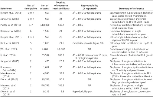
Table 1 List of published DMS studies assessing mutant growth rates in accordance with our statistical model, arranged by number of time points sampled

Reference No. of time points No. of mutants Total no. of sequence reads (millions) Reproducibility

(if reported) Summary of reference

Hietpaset al.(2013) 6 or 7 568 30 R2_¼₀_:_{95 for full replicates} _Bene_ﬁ_{cial single substitutions in Hsp90 of}

yeast under altered environments Jianget al.(2013) 6 or 7 568 34 R2_¼₀_:_{96 for full replicates} _{Interaction of expression and single}

substitutions on DFE of yeast Hsp90 Puchtaet al.(2016) 5–7 60,000 545.7 R2_¼₀_:₈₅ _{Network of epistatic interactions in yeast}

small nucleolar RNA Roscoeet al.(2013) 6 1,530 21 R2_¼₀_:_{93 for full replicates} _{Functional biophysics of single}

substitutions in ubiquitin of yeast Hietpaset al.(2011) 3 or 7 568 26 R2_¼₀_:_{82 for full replicates} _{DFE of single substitutions for a short}

region of Hsp90 in yeast

Banket al.(2015) 5 1,015 21.6 Credibility intervals (ﬁgure 6B) DFE of epistatic substitutions in Hsp90 of yeast

Wuet al.(2013) 3 .400 .0.002 NA Compensatory single substitutions for

neuraminidase mutant of inﬂuenza Liet al.(2016) 2 65,537 685.5 R2_¼₀_:_{997 mean across 15 pairs}

of biological replicates

Fitness landscape of a transfer RNA gene in yeast

Jianget al.(2015) 2 475 20.5 R2_¼₀_:_{92 for full replicates} _{Biophysics of single substitutions in}

inﬂuenza neuraminidase with antiviral Roscoe and

Bolon (2014)

2 1,617 30 R2_¼₀_:_{96 for full replicates} _{Biophysics of single ubiquitin substitutions}

on E1 activity and yeastﬁtness Melnikovet al.

(2014)

2 4,993 33.2 R2_¼₀_:_{90 for full replicates} _{Biophysics of single substitutions in APH}

(39)II inEscherichia coliwith antibiotics

Kimet al.(2013) 2 29,708 90.2 NA Biophysics of single substitutions in yeast

Deg1 protein degradation signal Melamedet al.

(2013)

2 110,745 186.5 NA Biophysics of single and multiple

substitutions in Pab1 RRM of yeast Klesmithet al.

(2015)

2 9,219 5.8 Reproducibility plot Biophysics of levoglucosan consumption rate inE. coli

(4)

Estimators for the selection coefﬁcients si are then

obtained from linear regression, based on log ratios of the number of sequencing readsniðtÞover the different sampling

time points (but see Banket al.2014, for a Bayesian Markov Chain Monte Carlo approach). The corresponding linear model can then be written as

yt¼Cþsitþet; (1)

whereytis the (transformed) observation variable,Cis a

con-stant (i.e., the intercept), andetdenotes the regression residual.

In the following, we derive an estimator that uses the log ratios of the number of reads of mutantiover the number of reads of the wild type as dependent variables in a linear re-gression. We call this method thewild-type(WT)approach. In Supplemental Material,File S2, we derive and analyze an al-ternative selection coefﬁcient estimator that is based on log ratios of the number of mutant reads with respect to the total number of sequencing reads, which we call the total(TOT) approach. This estimator has previously been used for detecting outliers within the experimental setup considered in Banket al. (2014).

Estimation of selection coefﬁcients^sWT

Ultimately, we want to calculate the mean of the log ratios of the number of sequencing reads for mutantiover the number of wild-type sequencing reads,E½logðniðtÞ=n1ðtÞÞBy noting thatniðtÞis

binomially distributed [for every mutanti2 f1;2;. . .;Kg] and using the Delta method (for derivation seeFile S1; see also Hurt 1976; Casella and Berger 2002), we derive

E "

log

niðtÞ þ1 n1ðtÞ þ1

#

¼ ElogðniðtÞ þ1Þ

2Elogðn1ðtÞ þ1Þ

logDpiðtÞ

2logDp1ðtÞ

¼log

piðtÞ p1ðtÞ

¼log ci c1 þsit

(2)

such that an estimator^sWT;iforsican be obtained by applying

the ordinary least-squares (OLS) method on the linear re-gression model

log

¼log ci c1

þsitþeWT;t; (3)

where eWT;t denotes the regression residual using the WT

approach (as opposed to the TOT approach; see also File S2). Note that the additive term within the logarithm ensures that the logarithm is always well deﬁned and was added solely for mathematical convenience.

Simulation of time-sampled deep sequencing data

To validate analytical results, we simulated time-sampled deep sequencing data (implemented in C++; available upon re-quest). We assumed that mutant libraries were created per-fectly, such that the initial population sizeciwas identical for all

mutants and, accordingly,piðt1Þ ¼1=Kfor alli¼1;2;. . .;K:

Selection coefﬁcients were independently drawn from a nor-mal distribution with mean 0 and standard deviation 0.1. To test the robustness of these assumptions we performed addi-tional simulations where initial population sizes were drawn from a log-normal distribution [i.e.,ci10Nð4;s¼0:5Þ]

reﬂect-ing empirical distributions of inferred initial population sizes. Furthermore, selection coefﬁcients were also drawn from a mixture distribution

si 2_Expð0jN ð0_:_02Þ;s¼0:1Þj if z¼0 if z¼1;

(4)

whereZBernoullið0:7Þ(Figure S1). For a given number of sampling time pointsTand sequencing depthD, the number of mutant sequencing reads ðn1ðtÞ;n2ðtÞ;. . .;nKðtÞÞ was

drawn from a multinomial distribution with parameters D andpðtÞfor each sampling point. Selection coefﬁcient esti-mates ð^siÞi¼2;...;K were then obtained by ﬁtting the linear

model by means of OLS. Finally, the accuracy of the param-eter estimates was assessed by computing the MSE,

MSE¼ 1 K21

XK

i¼2

ð^si2siÞ2; (5)

and the deviation (DEV)

DEV¼ 1 K21

XK

i¼2

ð^si2siÞ: (6)

Note that we have omitted the hat over the MSE and DEV for notational convenience. If not stated otherwise, statistics were calculated over 1000 simulated experiments for each set of parameters.

Data availability

The empirical data used in Figure 4 have been downloaded from Dryad, DOI: 10.5061/dryad.nb259 (data from Hietpas et al. 2013).

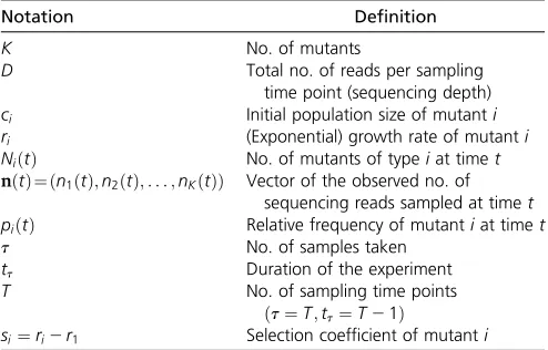
Table 2 Summary of notation and deﬁnitions

Notation Deﬁnition

K No. of mutants

D Total no. of reads per sampling

time point (sequencing depth)

ci Initial population size of mutanti ri (Exponential) growth rate of mutanti NiðtÞ No. of mutants of typeiat timet nðtÞ¼ðn1ðtÞ;n2ðtÞ;. . .;nKðtÞÞ Vector of the observed no. of

sequencing reads sampled at timet piðtÞ Relative frequency of mutantiat timet

t No. of samples taken

tt Duration of the experiment

T No. of sampling time points

ðt¼T;tt¼T21Þ

si¼ri2r1 Selection coefﬁcient of mutanti

(5)

Results and Discussion

The aim of this article is to provide a statistical framework fora priorioptimization of the experimental setup for future DMS studies. As such, our primary interest lies in the quantification of the MSE and its dependence on the experimental setup. Wefirst deduce analytical approximations for the variance and the MSE of the estimators for the selection coefficient and com-pare these with simulated data. We then derive approximate formulas for the length of the confidence interval of the esti-mates and the mean absolute error (MAE), which can be used to assess the expected precision of the estimates. For each of these steps, we discuss the consequences of relaxing some of the above assumptions along with potential extensions of the model. Finally, we apply our statistical framework to experimen-tal evolution data of 568 engineered mutations from Hsp90 in S. cerevisiaeand show that our model indeed captures the most prevalent source of error (i.e., error from sampling).

Approximation of the mean squared error

Generally, the MSE of an estimator^u(for parameteru) is given by

MSEð^uÞ ¼E h

ð^u2uÞ2i_¼_Var½_^

u þbiasð^uÞ2

(see section 7.3.1 of Casella and Berger 2002). Since E½eWT ¼0 (i.e., the mean of the regression residual is zero, implying that^sWT;iis an unbiased estimator;Figure S2), it is

sufﬁcient to analyze Var½^sWT;ito assess MSEð^sWT;iÞ:For ease

of notation, and since all results in the main text are derived using the wild-type approach, we omit the WT index from here on. Taking the variance of Equation 3 implies

Var "

log

#

¼Var½et; (7)

which, by applying the Delta method (seeFile S1) and using Equation S5 inFile S1together with Equations S4 and S6 in File S1can be approximated by

Var½et

DpiðtÞ

12piðtÞ

1þDpiðtÞ

2 þ

Dp1ðtÞ

12p1ðtÞ

1þDp1ðtÞ

2

22 DpiðtÞp1ðtÞ

1þDpiðtÞ

1þDp1ðtÞ

:

(8)

Note that the residuals are heteroscedastic [i.e., their variance is time dependent; the relative mutant frequenciespiðtÞ change

during the course of the experiment]. Hence, there is no gen-eral closed-form expression of the variance of^si:However, by

making the simplifying assumption of homoscedasticity [i.e., piðtÞ piðt1Þandp1ðtÞ p1ðt1Þfor allt], we obtain

Var½e Dpið12piÞ ð1þDpiÞ2

þDp1ð12p1Þ

ð1þDp1Þ2

22_ð1_þ Dpip1

DpiÞð1þDp1Þ

Dpið12piÞ ð1þDpiÞ2

þDp1ð12p1Þ

ð1þDp1Þ2

;

(9)

where the dependence on time has been dropped for ease of notation. Note that omitting the covariance term implicitly assumes that the number of mutantsK is sufﬁciently large (i.e.,piandp1 are small). We discuss the effect of assuming

homoscedastic error terms below. Equation 9 shows that Var½e decreases monotonically with increasing sequencing depth and increasing relative proportions of the wild-type and focal mutants.

Using existing theory on variances of slope coefﬁcients in a linear regression framework with homoscedastic error terms (e.g., see section 11.3.2 in Casella and Berger 2002), the variance of the selection coefﬁcient estimate is given by

MSEð^siÞ ¼Var½^si ¼

Var½e P_t

i¼1ðti2tÞ2 Dpið12piÞ

ð1þDpiÞ2

þDp1ð12p1Þ

ð1þDp1Þ2

! 1 P_t

i¼1ðti2tÞ2 ;

(10)

which is ourﬁrst main result.

Using that sampling times are assumed to be equally spaced, Equation 10 can further be rewritten as

MSEð^siÞ

þDp1ð12p1Þ

ð1þDp1Þ2

! 12

T3₂_T; (11)

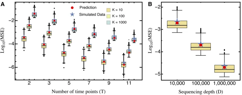
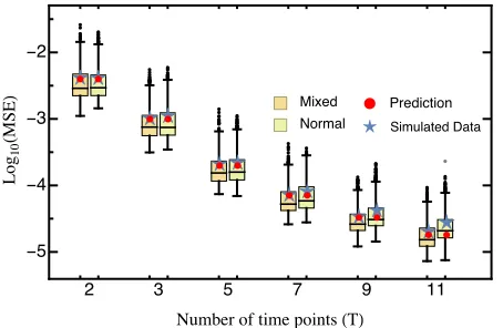
which shows that the MSE decreases cubically with the number of time points T (Figure 1). Thus, sampling addi-tional time points (i.e., taking more samples and thereby extending the duration of the experiment) drastically in-creases the precision of the measurement.

Our approximation generally performs very well across the entire parameter space. Although we assumed that the rela-tive abundance of all mutants remains roughly constant with time (i.e., neglecting that error terms are heteroscedastic), the (small) absolute error of our approximation remains con-stant across time points (Figure S3A). Deviations from ho-moscedasticity increase as more and later time points are sampled, as shown by the relative error (Figure S3B). This is also reﬂected by the deviation between the predicted MSE and the true average MSE obtained from the simulated data (Figure 1). For realistic experimental durations, however, compared to the experimental error (due to sampling) this approximation error is negligible.

Uneven sampling schemes: To obtain a closed formula for

the decay in the measurement error with the number of time samples T(Equation 11), we assumed equally spaced sampling times. The observed decay remains cubic relative to the number of time points also when samples are not taken at equally spaced time points. Furthermore, Equation 10 in-forms about the optimal sampling scheme to use to mini-mize measurement error: Forﬁxed sequencing depth and number of mutants, the MSE is minimized when the sum of squared deviations of the sampling times from their mean

(6)

is maximized. In other words, to minimize the measurement error one should sample in two sampling blocks, one at the beginning and another at the end of the experiment instead of sampling throughout the experiment, or, if time and re-sources allow, create full two-time-point replicates [e.g.,

t¼ ð0;1;5;6Þis better thant¼ ð0;2;4;6Þ;see also the in-teractive demonstration tool provided online].

Duration and sampling density of the experiment:

Equa-tion 11 implies that the MSE decreases cubically when both more samples are taken and the duration of the experiment is extended. However, extending the experiment indeﬁnitely is impossible, both because of experimental constraints and because secondary mutations will begin to affect the mea-surement. Hence, the possible duration of an experiment under a given condition may be a (ﬁxed) short time tt

(e.g.,,20 yeast generations forEMPIRIC). To separate the effects of taking more samplestfrom those of extending the duration of the experiment tt—which are combined inTin

the normal model setup (seeModel and Methods)—Equation 11 can be rewritten as

MSEð^siÞ

þDp1ð12p1Þ

ð1þDp1Þ2

!

12ðt21Þ tðtþ1Þt2

t: (12)

Thus, when the duration of the experimentttis held constant,

measurement error decays linearly ast (i.e., the number of sampling points) increases. Conversely, when extending the duration of experiment, the MSE decreases quadratically. This result suggests that the experimental duration should always be maximized under the constraints that mutants grow exponentially and population size is much smaller than the carrying capacity. How long both of these assumptions are met depends on each individual mutant’s selection coefﬁcient (or growth rate) and its initial frequency. Accordingly, there is

no universal“optimal”duration of the experiment. For exam-ple, the frequency of strongly deleterious mutations in the population generally decreases quickly, such that the phase where they show strict exponential growth is short and does not span the entire duration of the experiment. Furthermore, mutations might be lost from the population before the ex-periment is completed. Thus, when sampling two time points that extend over a long experimental time, growth rates for strongly deleterious mutations can be substantially over-estimated (see also Contribution of additional error: Data application).

Conversely, for mutations with small (i.e., wild-type-like) selection coefﬁcients, increasing the duration of the experi-ment considerably improves the precision of the estimates. Speciﬁcally, to infer deviations from the wild type’s growth rate the (expected) log ratio of the number of mutant se-quencing reads over the number of wild-type sese-quencing reads (i.e., the ratio of relative frequencies between mutant and wild-type abundance) needs to change consistently with time (i.e., either increase or decrease; Equation 2). However, changes in the log ratios will be small if the duration of the experiment is short, and even if there are slight shifts, se-quencing depthD needs to be large enough such that they are not washed out by sampling.

Thus, beyond the linear improvement on the MSE that comes with increasingt, sampling more time points can be an efficient strategy to capture the entire range of selection co-efficients (i.e., strongly deleterious and wild-type-like mu-tants). Specifically, sampling in two blocks (one at the beginning and another at the end of the experiment as sug-gested above) would allow using differenttt;depending on

the underlying selection coefﬁcient, which could be deter-mined by a bootstrap leave-p-out cross-validation approach (for details seeContribution of additional error: Data applica-tion). For example, theﬁrst sampling block could be used for

Figure 1 Comparison of the predicted mean squared error (Equation 10; red circles) and the average mean squared error (blue stars), obtained from 1000 simulated data sets for (A) different numbers of sampling time pointsTand mutantsK, for sequencing depthD¼100;000;and (B) different sequencing depthD, withﬁxedT¼5;K¼100:Boxes represent the interquartile range (i.e., the 50% C.I.), whiskers extend to the highest/lowest data point within the box61.5 times the interquartile range, and black and gray circles represent close and far outliers, respectively. Results are presented on log scale.

(7)

strongly deleterious mutations, whereas all sampled time points could be used for the remaining mutations, reducing error due to overestimation of strongly deleterious selection coefﬁcients and increasing statistical power to detect differ-ences from wild-type-like growth rates.

Library design and the number of mutants:Increasing the

number of mutantsKreduces the number of sequencing reads per mutant and hencepi;which explains the approximately

linear increase of the MSE with K(Figure 1). Crucially, we assumed that the initial mutant library was balanced, such that all mutants were initially present at equal frequencies. In practice this is hardly ever the case and previous analy-ses have shown that initial mutant abundances instead fol-low a log-normal distribution (Banket al.2014). Taking this into account, we ﬁnd that unbalanced mutant libraries, as expected from Equation 9, introduce an error due to the higher variance terms resulting from the generally lowerpi

(Figure S5). This error can be avoided by using the estimated relative mutant abundance,^pi;in Equation 9 (Figure S5).

The additional—although practically inevitable—error in-troduced by variance in mutant abundance indicates that library preparation is an important ﬁrst step for obtaining precise estimates. In fact, Equation 9 suggests that the mea-surement precision increases with the relative abundance of the wild type (such that the second term in Equation 9 decreases). However, this results in a trade-off because in-creasing wild-type abundance results in a decrease of the abundance of all other mutants, which leads to an increase of theﬁrst term in Equation 9. Assuming that increasing the relative abundance of the wild type reduces the relative abundance of all mutants equally (i.e., pi¼pj for all

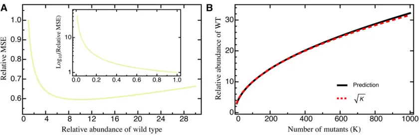
i;j2 f2;3;. . .;Kg), wefind that precision is maximized by increasing the wild-type abundance by a factor proportional topffiffiffiffiK(analytical result not shown; Figure 2). This way, the MSE can be reduced by 50% compared to the MSE with equal proportions of all mutants. Most importantly, however, if wild-type abundance is low (i.e., p11=K), the error

in-creases substantially (i.e.,.10-fold; see Figure 2A, inset).

Sequencing depth and its ﬂuctuations: The MSE

de-creases approximately linearly with the sequencing depth D (Figure 1), because the number of reads per mutant in-creases. As long asDis independent of the number of mutants K in the actual experiment, it can simply be treated as a rescaling parameter; hence, qualitative results are indepen-dent of the actual choice ofD. Similarly, the variance of the estimated MSE decreases approximately quadratically with sequencing depth and increases quadratically as the number of mutants increases (Figure 1).

Although we here treat the sequencing depthDas a con-stant parameter, it will in practice vary between sampling time points. Thus, D should rather be interpreted as the (expected) average sequencing depth taken over all time points. In particular, compared to aﬁxed sequencing depth, variance inDintroduces an additional source of error (due to increased heteroscedasticity), although deviations from the predicted to the observed mean MSE remain roughly identi-cal (Figure S6). Our model can also account for other forms of sampling. For example, if the sample taken from the bulk competition is known to be smaller than the sequencing depth, its size should be used asDin the precision estimates.

Shape of the underlying DFE: Our results remain

qualita-tively unchanged when selection coefﬁcients are drawn from differently shaped DFEs. The assumed normally distributed DFE corresponds to theoretical expectations derived from Fisher’s geometric model [assuming that the number of traits under selection is large (Martin and Lenormand 2006a; Tenaillon 2014)]. DFEs inferred from experimental evolu-tion studies, however, are typically characterized by an ap-proximately exponential tail of beneﬁcial mutations and a heavier tail of deleterious mutations (Eyre-Walker and Keightley 2007; Bank et al. 2014) that roughly follows a (displaced) gamma distribution (Martin and Lenormand 2006a; Keightley and Eyre-Walker 2010). To account for this expected excess of deleterious mutations in the DFE (reviewed by Bataillon and Bailey 2014), we used a mixture distribution that resulted in a highly skewed DFE. For this,

Figure 2 (A) The relative MSE as a function of the relative abundance of the wild type,i.e.,MSEðp1¼x=KÞ=MSEðp1¼1=KÞ;forK¼100:The inset

shows results forp1#1=K;where they-axis has been put on log scale. The abundance of all other (except the wild type) is assumed to scale proportionally. (B)

The relative wild-type abundance that minimizes the MSE as a function of the number of mutantsK. An explicit formula (given by the black line) is not shown due to complexity, but can well be approximated bypffiffiffiffiK:Either prediction is based on Equation 10. Other parameters:D¼100;000:

(8)

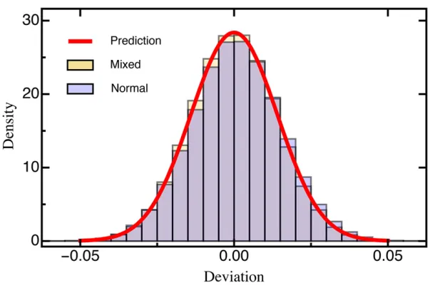
beneﬁcial mutations (s.0) were drawn from an exponential distribution and deleterious mutations were given by the ab-solute value drawn from a Gaussian distribution (Figure S1; see Model and Methods for details). Even with this highly skewed DFE, we did not ﬁnd changes in either the MSE (Figure S4) or the deviation (Figure 3), indicating that our results are robust across a range of realistic DFEs.

An alternative normalization: InFile S2, we analyze and

discuss an alternative estimation approach based on the log ratios of the number of mutant reads over the sequencing depth D (as opposed to a single reference/wild type) that was proposed in Banket al.(2014) and called the TOT ap-proach. Although the TOT approach can improve results for very noisy data (i.e., ifTorDis small;File S2, Figures A–D), its estimates are generally biased. The bias increases with the number of time points and overrides the smaller variance in residuals (see Equation 9 and File S2, Equation S8). Thus, application of the TOT approach is recommended only under special circumstances, e.g., under the suspicion of outlier measurements in the wild type (as in the case of Banket al. 2014).

Conﬁdence intervals, precision, and hypothesis testing

One way of quantifying the precision of the estimated selec-tion coefﬁcient is obtained using Jensen’s inequality (see sec-tion 6.6 of Williams 1991), which yields an upper bound for the MAE,

MAEð^siÞ#

ffiffiffiffiffiffiffiffiffiffiffiffiffi Var½^si p

ffiffiffiffiffiffiffiffiffiffiffiffiffiffiffiffiffiffiffiffiffiffiffiffiffiffiffiffiffiffiffiffiffiffiffiffiffiffiffiffiffiffiffiffiffiffiffiffiffiffiffiffiffiffiffiffiffiffiffiffiffiffiffiffiffiffiffiffiffiffiffiffiffiffiffiffiffiffiffiffiffiffiffiffiffiffiffi Dpið12piÞ

ð1þDpiÞ2

þDp1ð12p1Þ

ð1þDp1Þ2

! 1 P_t

i¼1ðti2tÞ2 v u u t ¼ ffiffiffiffiffiffiffiffiffiffiffiffiffiffiffiffiffiffiffiffiffiffiffiffiffiffiffiffiffiffiffiffiffiffiffiffiffiffiffiffiffiffiffiffiffiffiffiffiffiffiffiffiffiffiffiffiffiffiffiffiffiffiffiffiffiffiffiffiffiffiffiffiffiffiffi Dpið12piÞ

ð1þDpiÞ2

þDp1ð12p1Þ

ð1þDp1Þ2

! 12 T3₂_T

v u u

t _;

(13)

where, in the last line, we have again assumed that sampling times are equally spaced. Thus, the MAE is simply the square root of the MSE.

Alternatively, using central limit theorem arguments (Rice 1995), it can be shown that for aﬁxed mutantithe estimated selection coefﬁcient^siasymptotically follows a normal

distri-bution (Figure 3 andFigure S2). The upper and lower bounds of theð12aÞ-conﬁdence interval with signiﬁcance levelafor siare then given by

C:I:ð^siÞ ¼^si6

ffiffiffiffiffiffiffiffiffiffiffiffiffi Var½^si p

z12a=2; (14)

wherez12a=2denotes theð12a=2Þquantile of the standard

normal distribution. The length of the ð12aÞ-conﬁdence interval,Lð12aÞ;can be used as an intuitivea priorimeasure

for the precision of the estimated selection coefficient. For-mally, let L12a¼2 ffiffiffiffiffiffiffiffiffiffiffiffiffiVar½^si

p

z12a=2 denote the length of the

ð12aÞ-conﬁdence interval. Setting a¼0:05 and using Equation 10, we obtain the approximation

L0:954

ffiffiffiffiffiffiffiffiffiffiffiffiffiffiffiffiffiffiffiffiffiffiffiffiffiffiffiffiffiffiffi K

D 2 P_t

i¼1ðti2tÞ2 s

20

ffiffiffiffiffiffiffiffiffiffiffiffiffiffiffiffiffiffiffiffiffi K DðT3₂_TÞ

s

; (15)

where we assumed z0:9752: Equation 15 shows that the

sequencing depth D and the number of mutants K are in-versely proportional. Similar to Equation 10, the number of time pointsTenters cubically.

Furthermore, Equation 14 can be used to deﬁne the upper and lower bounds of the region of rejection of a two-sided Z-test with, for instance, null hypothesissi¼0 (or more

gen-erally any other null hypothesissi¼u). TheZ-statistic is then

given by

Z¼ ^sffiffiffiffiffiffiffiffiffiffiffiffiffii2u Var½^si

p (16)

(see Chap. 8 in Sprinthall 2014). This statistic can be applied to existing data to test whether a mutant has an effect

Figure 3 Histogram of the deviation (Equation 6)

be-tween the estimated and true selection coefﬁcients drawn from either a normal distribution or a mixture distribution (for details seeModel and Methods) based on 1000 sim-ulated data sets each. The red line is the prediction based on Equation 10. Other parameters:T¼5;D¼100;000; K¼100:

(9)

different from the wild type. In addition, we can use this statistic to determine the maximum achievable statistical res-olution of a planned experiment.

Optimization of experimental design

Equation 10 suggests that the measurement error modeled here could in theory be eliminated entirely by sampling (in-ﬁnitely) many time points. In practice, the attainable resolu-tion of the experiment is also limited by technical constraints imposed by the experimental details and by sequencing error and by the available manpower and budget. To further im-prove the experimental design taking the latter two factors into account, we can integrate our approach into an optimi-zation problem, using a cost functionCa;b;Ctt;KðD;tt;tÞ:As an example, we deﬁne

C_a;b;Ct_t;KðD;t;ttÞ ¼tt3Cttþt3fðDÞ

þa3MSEKðD;tt;tÞb; (17)

where Ctt denotes the personnel costs over the dura-tion of the experiment, fðDÞ denotes the sequencing costs per sampled time point, andaandbscale the as-sociated error costs given by Equation 12 (Boyd and Vandenberghe 2004). The optimization problem is solved by minimizing

C_a;b;C_ttðD;tt;tÞ (18a)

under constraints

2#t#tmax (18b)

t_t;min#tt#tt;max (18c)

Dmin#D#Dmax (18d)

MSEKðD;tt;tÞ#MSEmax; (18e)

which yields the maximum tolerable error MSEmax while

minimizing the total experimental costs. An illustrative ex-ample is given inFile S3.

Contribution of additional error: Data application

An important limitation of our model is that it does not consider additional sources of experimental error. Therefore, any results presented here should be interpreted as upper limits of the attainable precision. In particular, sequencing error (dependent on the sequencing platform and protocol used) is expected to affect the precision of measurements. However, if the additional error is nonsystematic (i.e., ran-dom), it will not change the results qualitatively, but solely add an additional variance to the measurement.

To assess the influence of additional error sources on the validity of our statistical framework, we reanalyzed a data set of 568 engineered mutations from Hsp90 in S. cerevisiae grown in standard laboratory conditions (i.e., 30°; for details see Banket al.2014). We estimated the initial population size and the selection coefficient for each mutant, using the linear-regression framework discussed here. With respect to the experimental parameters (i.e., number and location of sampling points, sequencing depth) and our proposed model, we simulated 1000 bootstrap data sets. We assessed the ac-curacy of our selection coefficient estimates by calculating the MSE between the selection coefficient estimates obtained from the bootstrap data sets and those obtained from the experimental data, which serve as a reference for the“true” (but unknown) selection coefficient. To quantify the effect of the number of sampling time points, we used a leave-p-out cross-validation approach, successively dropping sampling time points (Geisser 1993).

For the complete data set, our prediction holds only when the number of time points considered is small. Conversely, with more than four time samples, the MSE even slightly increases with the number of sampling points (Figure 4, in-set). However, when strongly deleterious mutations (i.e.,

Figure 4Comparison of the predicted mean squared error (Equation 10; red) against the average mean squared error (blue stars) obtained from 1000 cross-validation data sets. Only mutants with an estimated selection coefﬁcient larger than the intermediate between the estimated mean syno-nym and the estimated mean stop codon selection coefﬁ -cient were considered. The inset shows the MSE calculated for all mutants. The MSE is presented on log scale. Other parameters:t¼ ð4:8;7:2;9:6;12;16:8;26:4;36Þ;

DFigure¼ ð474;931;636;257;873;827;1;513;392;424;182;

443;739;452;326Þ;DInset¼ ð654;311;820;301;1;046;169;

1;726;516;469;855;464;070; 463;363Þ; KFigure ¼ 400; KInset¼568:Alternatively, in the presence of strongly

dele-terious mutants a Poisson regression may be used for esti-mating growth rates (seeFigure S7).

(10)

those with a selection coefﬁcient closer to that of the average stop codon than to the wild type; see also Banket al.2014) are excluded from the analysis, the MSE is very well pre-dicted by Equation 10 for any number of time points (Figure 4). Two model violations may well explain the observed pattern when deleterious mutations are included. First, the frequency of strongly deleterious mutations in the population decreases quickly and does not show strictly exponential growth (ﬁgure S2 in Banket al.2014), especially for later time points. Second, these mutations might not be present in the population over the entire course of the experiment. Sequenc-ing error will then create a spurious signal, feignSequenc-ing and extend-ing their “presence,” thus biasing the results. The bootstrap approach utilized here could in principle be used to determine the time points that should be considered for the estimation of strongly deleterious mutations and to generally test for model violations. Indeed, Figure 4 demonstrates that our model cap-tures the most prevalent source of error (i.e., error from sam-pling) when strongly deleterious mutations are excluded.

Conclusion

The advent of sophisticated biotechnological approaches on a single-mutation level, combined with the continual improve-ment and reduction in costs of sequencing, presents us with an unprecedented opportunity to address long-standing ques-tions about mutational effects and the shape of the distribu-tion ofﬁtness effects. An additional step toward optimizing results receives little attention: By systematically invoking statistical considerations ahead of empirical work, it is possi-ble to quantify and maximize the attainapossi-ble experimental power while avoiding unnecessary expenses, regarding both ﬁnancial and human resources. Here, we present a thorough statistical analysis that results in several straightforward, general predictions and rules of thumb for the design of DMS studies, which can be applied directly to future exper-iments using a free interactive web tool provided online (https://evoldynamics.org/tools). We emphasize here three important and general rules that emerged from the analysis:

1. Increasing sequencing depth and the number of replicate experiments is good, but adding sampling points together with increasing the duration of the experiment is much better for accurate estimation of small-effect selection coefﬁcients.

2. Preparation of a balanced library is the key to good results. The quality of selection coefﬁcient estimates strongly depends on the abundance of the reference genotype: Always ensure that the frequency of the reference geno-type is . 1=K—“less is a mess.”

3. Clustering sampling points at the beginning and the end of the experiment increases experimental power and allows the efﬁcient and precise assessment of the entire range of the distribution ofﬁtness effects.

Although the statistical advice presented here is limited to experimental approaches that fulﬁll the requirements listed in the Introduction and focuses on the error introduced through

sam-pling, our work highlights the promises that lie in long-term collaborations between theoreticians and experimentalists com-pared to the common practice ofpost hocstatistical consultation.

Acknowledgments

We thank Ivo Chelo, Inês Fragata, Isabel Gordo, Kristen Irwin, Adamandia Kapopoulou, and Nicholas Renzette for helpful discussion and comments on earlier versions of this manuscript. This project was funded by grants from the Swiss National Science Foundation and a European Research Council starting grant (to J.D.J.).

Literature Cited

Bank, C., R. T. Hietpas, A. Wong, D. N. Bolon, and J. D. Jensen, 2014 A Bayesian MCMC approach to assess the complete dis-tribution of ﬁtness effects of new mutations: uncovering the potential for adaptive walks in challenging environments. Genetics 196: 841–852.

Bank, C., R. T. Hietpas, J. D. Jensen, and D. N. Bolon, 2015 A systematic survey of an intragenic epistatic landscape. Mol. Biol. Evol. 32: 229–238.

Bataillon, T., and S. F. Bailey, 2014 Effects of new mutations onﬁtness: insights from models and data. Ann. N. Y. Acad. Sci. 1320: 76_–92. Bernet, G. P., and S. F. Elena, 2015 Distribution of mutational ﬁtness effects and of epistasis in the 5₉untranslated region of a plant RNA virus. BMC Evol. Biol. 15: 1_–13.

Boucher, J. I., D. N. A. Bolon, and D. S. Tawﬁk, 2016 Quantifying and understanding theﬁtness effects of protein mutations: Lab-oratoryvs.nature. Protein Sci. 25(7): 1219–26.

Boyd, S., and L. Vandenberghe, 2004 Convex Optimization. Cam-bridge University Press, CamCam-bridge, UK/London/New York. Casella, G., and R. L. Berger, 2002 Statistical Inference, Vol. 2.

Duxbury Press, Paciﬁc Grove, CA.

Charlesworth, D., B. Charlesworth, and M. T. Morgan, 1995 The pattern of neutral molecular variation under the background selection model. Genetics 141: 1619–1632.

Chen, F., S. M. Pruett-Miller, Y. Huang, M. Gjoka, K. Dudaet al., 2011 High-frequency genome editing using ssDNA oligonucle-otides with zinc-ﬁnger nucleases. Nat. Methods 8: 753–755. Connallon, T., and A. G. Clark, 2015 The distribution ofﬁtness

effects in an uncertain world. Evolution 69: 1610–1618. Eyre-Walker, A., 2010 Genetic architecture of a complex trait and

its implications for_ﬁtness and genome-wide association studies. Proc. Natl. Acad. Sci. USA 107: 1752_–1756.

Eyre-Walker, A., and P. D. Keightley, 2007 The distribution of ﬁtness effects of new mutations. Nat. Rev. Genet. 8: 610–618. Firnberg, E., J. W. Labonte, J. J. Gray, and M. Ostermeier, 2014 A

comprehensive, high-resolution map of a gene’s ﬁtness land-scape. Mol. Biol. Evol. 31: 1581–1592.

Fowler, D. M., and S. Fields, 2014 Deep mutational scanning: a new style of protein science. Nat. Methods 11: 801–807. Fowler, D. M., C. L. Araya, S. J. Fleishman, E. H. Kellogg, J. J.

Stephany et al., 2010 High-resolution mapping of protein sequence-function relationships. Nat. Methods 7: 741–746. Frenkel, E. M., B. H. Good, and M. M. Desai, 2014 The fates of

mutant lineages and the distribution ofﬁtness effects of beneﬁ -cial mutations in laboratory budding yeast populations. Genetics 196: 1217–1226.

Geisser, S., 1993 Predictive Inference (Chapman & Hall/CRC Monographs on Statistics & Applied Probability). Taylor & Francis. New York, NY.

(11)

Gerrish, P. J., and R. E. Lenski, 1998 The fate of competing beneﬁcial mutations in an asexual population. Genetica 102/103: 127–144. Gillespie, J. H., 1983 A simple stochastic gene substitution model.

Theor. Popul. Biol. 23: 202–215.

Gordo, I., and P. R. A. Campos, 2013 Evolution of clonal popula-tions approaching aﬁtness peak. Biol. Lett. 9: rsbl20120239. Halligan, D. L., and P. D. Keightley, 2010 Spontaneous mutation

accumulation studies in evolutionary genetics. Annu. Rev. Ecol. Evol. Syst. 40: 151–172.

Hietpas, R., B. Roscoe, L. Jiang, and D. N. A. Bolon, 2012 Fitness analyses of all possible point mutations for regions of genes in yeast. Nat. Protoc. 7: 1382_–1396.

Hietpas, R. T., J. D. Jensen, and D. N. A. Bolon, 2011 Experimental illumination of a_ﬁtness landscape. Proc. Natl. Acad. Sci. USA 108: 7896–7901.

Hietpas, R. T., C. Bank, J. D. Jensen, and D. N. A. Bolon, 2013 Shiftingﬁtness landscapes in response to altered envi-ronments. Evolution 67: 3512–3522.

Hurt, J., 1976 Asymptotic expansions of functions of statistics. Appl. Math. 21: 444–456.

Imhof, M., and C. Schlötterer, 2001 Fitness effects of advanta-geous mutations in evolvingEscherichia colipopulations. Proc. Natl. Acad. Sci. USA 98: 1113–1117.

Jacquier, H., A. Birgy, H. Le Nagard, Y. Mechulam, E. Schmittet al., 2013 Capturing the mutational landscape of the beta-lactamase tem-1. Proc. Natl. Acad. Sci. USA 110: 13067–13072.

Jensen, J. D., K. R. Thornton, and P. Andolfatto, 2008 An approx-imate Bayesian estimator suggests strong, recurrent selective sweeps in Drosophila. PLoS Genet. 4: e1000198.

Jiang, L., P. Mishra, R. T. Hietpas, K. B. Zeldovich, and D. N. A. Bolon, 2013 Latent effects of hsp90 mutants revealed at re-duced expression levels. PLoS Genet. 9: e1003600.

Jiang, L., P. Liu, C. Bank, N. Renzette, K. Prachanronaronget al., 2015 A balance between inhibitor binding and substrate process-ing confers inﬂuenza drug resistance. J. Mol. Biol. 428: 538–553. Jinek, M., K. Chylinski, I. Fonfara, M. Hauer, J. A. Doudna et al., 2012 A programmable dual-RNA–guided DNA endonuclease in adaptive bacterial immunity. Science 337: 816–821. Joung, J. K., and J. D. Sander, 2013 TALENS: a widely applicable

technology for targeted genome editing. Nat. Rev. Mol. Cell Biol. 14: 49–55.

Keightley, P. D., and A. Eyre-Walker, 2010 What can we learn about the distribution ofﬁtness effects of new mutations from DNA sequence data? Philos. Trans. R. Soc. B 365: 1187–1193. Kim, I., C. R. Miller, D. L. Young, and S. Fields, 2013

High-throughput analysis ofin vivoprotein stability. Mol. Cell. Pro-teomics 12: 3370_–3378.

Kimura, M., 1979 Model of effectively neutral mutations in which selective constraint is incorporated. Proc. Natl. Acad. Sci. USA 76: 3440_–3444.

Klesmith, J. R., J.-P. Bacik, R. Michalczyk, and T. A. Whitehead, 2015 Comprehensive sequence-ﬂux mapping of a levoglucosan utilization pathway in E. coli. ACS Synth. Biol. 4: 1235–1243. Kowalsky, C. A., J. R. Klesmith, J. A. Stapleton, V. Kelly, N. Reichkitzer

et al., 2015 High-resolution sequence-function mapping of full-length proteins. PLoS ONE 10: 1–23.

Li, C., W. Qian, C. J. Maclean, and J. Zhang, 2016 Theﬁtness landscape of a tRNA gene. Science 352: 837–840.

Martin, G., and T. Lenormand, 2006a A general multivariate ex-tension of Fisher’s geometrical model and the distribution of mutationﬁtness effects across species. Evolution 60: 893–907. Martin, G., and T. Lenormand, 2006b Theﬁtness effect of

muta-tions in stressful environments: a survey in the light ofﬁtness landscape models. Evolution 60: 2413_–2427.

Melamed, D., D. L. Young, C. E. Gamble, C. R. Miller, and S. Fields, 2013 Deep mutational scanning of an rrm domain of the Saccha-romyces cerevisiae poly(a)-binding protein. RNA 19: 1537_–1551.

Melnikov, A., P. Rogov, L. Wang, A. Gnirke, and T. S. Mikkelsen, 2014 Comprehensive mutational scanning of a kinasein vivoreveals substrate-dependentﬁtness landscapes. Nucleic Acids Res. 42: e112. Ohta, T., 1977 Molecular Evolution and Polymorphism. National

Institute of Genetics, Mishima, Japan.

Ohta, T., 1992 The nearly neutral theory of molecular evolution. Annu. Rev. Ecol. Syst. 23: 263–286.

Olson, C. A., N. C. Wu, and R. Sun, 2014 A comprehensive bio-physical description of pairwise epistasis throughout an entire protein domain. Curr. Biol. 24: 2643–2651.

Orr, H. A., 1998 The population genetics of adaptation: the dis-tribution of factors_ﬁxed during adaptive evolution. Evolution 52: 935_–949.

Orr, H. A., 2005a The genetic theory of adaptation: a brief history. Nat. Rev. Genet. 6: 119–127.

Orr, H. A., 2005b Theories of adaptation: what they do and don’t say. Genetica 123: 3–13.

Orr, H. A., 2009 Fitness and its role in evolutionary genetics. Nat. Rev. Genet. 10: 531–539.

Puchta, O., B. Cseke, H. Czaja, D. Tollervey, G. Sanguinettiet al., 2016 Network of epistatic interactions within a yeast snoRNA. Science 352: 840–844.

Rice, D. P., B. H. Good, and M. M. Desai, 2015 The evolutionarily stable distribution ofﬁtness effects. Genetics 200: 321–329. Rice, J., 1995 Mathematical Statistics and Data Analysis(Duxbury

Advanced Series, Ed. 1.). Duxbury Press. Belmont, CA. Rokyta, D. R., P. Joyce, S. B. Caudle, and H. A. Wichman, 2005 An

empirical test of the mutational landscape model of adaptation using a single-stranded DNA virus. Nat. Genet. 37: 441–444. Roscoe, B. P., and D. N. A. Bolon, 2014 Systematic exploration of

ubiquitin sequence, e1 activation ef_ﬁciency, and experimental ﬁtness in yeast. J. Mol. Biol. 426: 2854_–2870.

Roscoe, B. P., K. M. Thayer, K. B. Zeldovich, D. Fushman, and D. N. A. Bolon, 2013 Analyses of the effects of all ubiquitin point mutants on yeast growth rate. J. Mol. Biol. 425: 1363–1377. Rozen, D. E., J. A. G. M. de Visser, and P. J. Gerrish, 2002 Fitness

effects of ﬁxed beneﬁcial mutations in microbial populations. Curr. Biol. 12: 1040–1045.

Sarkisyan, K. S., D. A. Bolotin, M. V. Meer, D. R. Usmanova, A. S. Mishinet al., 2016 Localﬁtness landscape of the greenﬂ uo-rescent protein. Nature 533: 397–401.

Sawyer, S. A., R. J. Kulathinal, C. D. Bustamante, and D. L. Hartl, 2003 Bayesian analysis suggests that most amino acid replace-ments in Drosophila are driven by positive selection. J. Mol. Evol. 57: S154–S164.

Schneider, A., B. Charlesworth, A. Eyre-Walker, and P. D. Keightley, 2011 A method for inferring the rate of occurrence and_ﬁtness effects of advantageous mutations. Genetics 189: 1427_–1437. Sousa, A., S. Magalhaes, and I. Gordo, 2012 Cost of antibiotic resistance

and the geometry of adaptation. Mol. Biol. Evol. 29: 1417_–1428. Sprinthall, R. C., 2014 Basic Statistical Analysis, Ed. 9. Pearson.

New York, NY.

Tenaillon, O., 2014 The utility of Fisher’s geometric model in evolutionary genetics. Annu. Rev. Ecol. Evol. Syst. 45: 179–201. Whitehead, T. A., A. Chevalier, Y. Song, C. Dreyfus, S. J. Fleishman et al., 2012 Optimization of affinity, specificity and function of designed influenza inhibitors using deep sequencing. Nat. Bio-technol. 30: 543–548.

Williams, D., 1991 Probability with Martingales(Cambridge Math-ematical Textbooks). Cambridge University Press, Cambridge, UK/London/New York.

Wu, N. C., A. P. Young, S. Dandekar, H. Wijersuriya, L. Q. Al-Mawsawi et al., 2013 Systematic identiﬁcation of h274y compensatory mutations in inﬂuenza A virus neuraminidase by high-throughput screening. J. Virol. 87: 1193_–1199.

Communicating editor: D. M. Weinreich

(12)

GENETICS

Supporting Information www.genetics.org/lookup/suppl/doi:10.1534/genetics.116.190462/-/DC1

A Statistical Guide to the Design of Deep Mutational

Scanning Experiments

Sebastian Matuszewski, Marcel E. Hildebrandt, Ana-Hermina Ghenu, Jeffrey D. Jensen, and Claudia Bank

(13)

- - -

(14)

(15)

-( )

(

)

-( )

= =

=

(16)

-( )

(

)

(17)

-( )

(

)

= /

( = )

-( )

(

)

Figure S5– The mean squared error obtained from 1,000 simulated data sets with a fixed initial population sizecicompared to that wherecihas been drawn from a log-normal distribution.

InAthe prediction (eq.10; red) is based on ˆpi, i.e., the estimated relative abundance of mutantisuch that it can be referenced against the empirical average MSE (blue stars).B

compares the empirical average MSE (solid line) against the predicted MSE with a balanced mutant library (i.e.,p=1/K; black) and an uneven mutant library (i.e.,

(18)

-( )

(

)

(19)

-( )

(

)

-( )

(

)

-( )

(

)

(20)

Supporting Information

File S1. Derivation of the Delta method

In this Supporting Information we will briefly motivate and introduce the delta method and derive the equations in the main text. Consider a generic random variable Xwith finite second moment and smooth function f : R _! R. If f is non-linear E[f(X)] =f(E[X])does in general no longer hold such that fandE[•]can no longer be interchanged. However, an approximate

result can be obtained by Taylor-expandingfaroundE[X]up to the second order such that

E[f(X)]⇡E⇥f(E[X]) + f0₍_E_[_X_])(_X _E_[_X_])

+1

2f00(E[X])(X E[X])2]

=f(E[X]) +1

2f00(E[X])V(X).

(S1)

This approach is called the Delta-method or method of error propagation (Hurt 1976;Oehlert 1992;Casella and Berger 2002). Thus, forX⇠Bin(D,p)and f(x) =log(1+x), the expectation off(X)can be approximated as

E[log(X+1)]⇡log(1+Dp) 1

2

Dp(1 p)

(1+Dp)2 ⇡log(Dp), (S2)

which is used in equation (2) in the main text. Note that the approximation induces a small error. However, for fixedpthis distortion is of orderO(D 1₎_{, which is generally negligible if}_D_{is large (i.e., when the sequencing depth is large).}

Analogously, we can calculate the variance off(X)as

Var[f(X)]⇡ f0₍_E_[_X_])2_Var_[_X_]_, _(S3)

which again forX⇠Bin(D,p)andf(x) =log(1+x)becomes

Var[log(X+1)]⇡ Dp(1 p)

(1+Dp)2, (S4)

which is used in equation (9) and (10) in the main text.

Similarly, letg:R2_!Rbe a smooth function andX1,X2denote two square integrable random variables. Taylor-expanding up to the first order and taking variances yields

Var[g(X1,X2)]⇡∂1g(E[X1],E[X2])2Var[X1] +∂2g(E[X1],E[X2])2Var[X2] +2∂1g(E[X1],E[X2])∂2g(E[X1],E[X2])Cov[X1,X2],

(S5)

which is used for the derivation of equation (9) and (10) in the main text. Furthermore, ifx1andx2denote two realizations of the same multinomial, the covariance betweenx1andx2are given by

Cov[x1,x2] = Dp1p2, (S6)

which is again used in equation (9) and (10) in the main text.

(21)

File S2. The Total Approach

In this Supporting InformationFile S2we derive and analyze an alternative estimator of selection coefficient to the one proposed in the main text. Unlike the WT approach this estimator is based on the log-ratios of the number of mutant reads with respect to thetotalnumber of sequencing reads (i.e., sequencing depth) and which is thus called thetotal approach(TOT). This estimator has previously been used for detecting outliers in time-sampled deep-sequencing bulk completion data (Banket al.2014) and proved to be more robust than the WT approach. Analogous to the main text we will first analyse and discuss the statistical properties of selection coefficient estimator based on the TOT approach and then compare its performance to the WT approach. Finally, we will end by giving rough guidelines when to prefer one over the other approach.

Statistical analysis of the TOT approachIn contrast to the WT approach the TOT approach is based on the log-ratios of the number of mutant reads with respect to the sequencing depthD, such that a linear model can be written as

log

✓_n i(t) +1

D

◆

=log ci

ÂKj=1cj !

+log(pi(t)) +#TOT,t

=log ci

ÂKj=1cj !

+log

0

@ exp(rit)

ÂK_j=1exp

⇣

rjt ⌘

1 A+#TOT,t

⇡log ci

ÂKj=1cj !

+sit+#TOT,t, (S7)

where the approximation assumes thatrj⇡1 for all mutantsK.

Then, with a calculation analogous to the one in the main text, we obtain

Var[#TOT,t]⇡ Dp₍₁i(₊t)(_Dp1 pi(t))

i(t))2 . (S8)

Again assuming that residuals are homoscedastic, i.e., thatpi(t)⇡pi(t1)for allt, we have

Var⇥sˆTOT,i⇤⇡ Dp₍₁i(₊t)(_Dp1 pi(t)) i(t))2

1 Ât

i=1(ti ¯t)2

= Dpi(t)(1 pi(t)) (1+Dpi(t))2

12

T3 _T. (S9)

However, the approximation used in equation (S7) induces a systematic error, such that E[#TOT,t]6=0 meaning that ˆsTOT,iis generally biased as can be seen from FigureAand FigureB.

-( )

(

)

-( )

(

)

/

Figure A– The average mean squared error (blue star) obtained from 1,000 simulated data sets forAdifferent numbers of sampling time pointsTcompared against the analytical prediction with (red) and without (purple) accounting for the estimation bias as given by equationS15andS9, respectively.Bfor different numbers of sequencing readsDwithT=5. Boxes represent the interquartile range (i.e., the 50% C.I.), whiskers extend to the highest/lowest data point within the box±1.5 times the interquartile range, and black and gray circles represent close and far outliers, respectively. Results are presented on log-scale. Other parameters:D=100,000,K=100.

(22)

-( )

-Figure B–AComparison of the deviation (eq.6) of the true and estimated selection coefficient as obtained by the WT and TOT approach, calculated from 1,000 simulated data sets for different numbers of sampling time pointsT.BHistogram of the deviation (eq.6) between the estimated and true selection coefficients based on 1,000 simulated data sets using the TOT approach withT=5. The red line is a normal distribution centered around the empirical mean and variance given by the square root of equation (S9). Other parameters:

D=100,000,K=100.

To quantify this bias, we will now derive an approximation based on the Delta method (see Supporting InformationFile S1). Rewriting equation (S7) we obtain

log

✓_n i(t) +1

D

◆

=log ci

ÂKj=1cj !

+log

0

@ exp(rit)

ÂKj=1exp

⇣

rjt ⌘

1 A+#TOT,t

=log ci

ÂKj=1cj !

+sit+log 0 @

_Â

K

j=1 exp⇣sjt

⌘1

A+et, (S10)

where(et)t=1,...,T are independent with mean zero, and#TOT,t = log ⇣

ÂKj=1exp

⇣

sjt ⌘⌘

+et. For ease of notation we will define yt:=log

⇣_n

i(t)+1

D ⌘

andXt:= log ⇣

ÂKj=1exp

⇣

sjt ⌘⌘

, and use the fact that the slope coefficient of a simple linear regression can be expressed as

ˆ

sTOT= Â t

i=1(ti ¯t)yt

Ât

i=1(ti ¯t)2. (S11)

Definingwti :=

(ti ¯t)y_ti

Ât

l=1(tl ¯t)2, and using thatÂ

t

j=1wtj =0,Âtj=1wtjtj=1 and E[et] =0, we obtain

bias ˆsTOT,i =E⇥sˆTOT,i si⇤

=E

2 4

_Â

t

j=1wtj#t

3 5

= t

Â

j=1wtj E[#t]

= t

Â

j=1wtj EhXtj

i

. (S12)

Note that in order to derive an explicit formula for the bias, the distribution of the(si)i=2,...,Kneeds to be specified. In accordance with our simulation assumptions, we consider the case where thesj i.⇠ Ni.d (0,s). Hence, the random variablesYti :=ÂKj=2exp(sjti)are sums of i.i.d. log-normal random variables with the first three moments given by

E[Yti] = (K 1)exp

⇣

(sti)2/2 ⌘

Var[Yti] = (K 1)(exp

⇣

(sti)2 ⌘

1)exp⇣(sti)2 ⌘

Eh(Yti E[Yti])3

i

=exp⇣3(sti)2/2 ⌘ ⇣

exp⇣(sti)2 ⌘

1⌘2⇣exp⇣(sti)2 ⌘

+2⌘

(23)

SinceXti = log(Yti), we have that Taylor-expanding up to the third order and taking expectations yields

E[Xti]⇡ log(K 1) +

e(sti)2 1

2(K 1)

(sti)2 2

1 3(K 1)2

⇣

exp⇣(sti)2 ⌘

1⌘2⇣exp⇣(sti)2 ⌘

+2⌘. (S13)

Finally, combining equations (S12) and (S13) and using thatÂt

i=1wti =0 yields

bias(sˆTOT,i) =

t

Â

j=1 wtj

0 @exp

⇣

(stj)2 ⌘

1 2(K 1)

(stj)2 2

1 3(K 1)2

⇣

exp⇣(stj)2 ⌘

1⌘2⇣exp⇣(stj)2 ⌘

+2⌘

1

A. (S14)

Note that the accuracy of the approximation strongly depends ons,tandttpotentially because of the local validity implied by the Taylor approximation breaking down. In particular, for smallsandT(i.e.,s0.1,t7 andtt 7) yields a reasonable prediction of the bias (Figs.A,C).

Thus, by combining equations (S9) and (S14) we obtain

MSE ˆsTOT,i =Var[sTOTˆ ] +bias(sTOT,ˆ i)

⇡ Dpi(t)(1 pi(t))

(1+Dpi(t))2

1

Ât

j=1

⇣

tj ¯t ⌘2

+

Â

t

j=1 wtj

0 @exp

⇣

(stj)2 ⌘

1 2(K 1)

(stj)2 2

1 3(K 1)2

⇣

exp⇣(stj)2 ⌘

1⌘2⇣exp⇣(stj)2 ⌘

+2⌘

1

A (S15)

While comparing equations (9) and (S9) shows that Var⇥sˆTOT,i⇤<Var⇥sˆWT,i⇤(with identicalT,Dandpi), the bias clearly limits the use of the TOT approach. In particular, the bias is strongest whenT(and in particulartt) is large and/or only a few mutants were considered (i.e.,Kis low relative toD). Similarly, increasingDdoes not improve the mean MSE by much (Fig.A).

= = = -( ) ( )

Figure C– Comparison of the predicted mean squared error (eq.S15; red) against the average mean squared error (blue star) obtained from 1,000 simulated data sets for different numbers of sampling time pointsTand mutantsK. Other parameters:D=100,000.

Comparison of the WT and TOT approachComparing the TOT approach to the WT approach (Fig.D) shows that the former only outperforms the latter when stochastic forces (induced by the multinomial sampling and only a few sampling time points) are large (i.e., whenDandTare small, andKis big) – in other words whenever there were problems with obtaining the data. This also shows up by the generally reduced variance of the MSE when increasingKor decreasingD(Figs.A,C,D). This is due to the fact that calculating the log-ratios with respect to the sequencing depthDintroduces a “saturation effect” such that the log-ratios are non-linear intas if the mutants no longer grow exponentially (comparable to deceleration and saturation phase described inHallet al.2014). In line with our observations (Figs.A,C,D), this effect is strongest ifKis small and/orTis large (and the duration of the experiment is long), i.e., ifpibecomes large such that the log-ratios saturate. Accordingly, the bias also strongly depends on the variance of the DFE and thus on the environment. If mutants can generally grow faster, i.e., if the variance in the DFE is high, the log-ratios will start to become saturated even earlier (i.e., with smallerT). The overall effect is that selection coefficient estimates will be less extreme, i.e., large positive selection coefficients (strongly beneficial mutants) will be underestimated whereas large negative selection coefficients (strongly deleterious mutants) will be overestimated. Still, when the wild type is systematically misestimated (due to some non-random error in the experiment) or if the the wild type is rare (see also Fig2) the TOT approach might outperform the WT approach. Furthermore, when applied for detecting outliers – where this approach has been proposed initially and proved to be more robust (Banket al.2014) – only the TOT approach is able to detect potential outliers in the wild type. In particular, when outliers in the wild type remain undetected they will introduce a bias in the estimated selection coefficients for all other mutants. Accordingly,

(24)

calculating the log-ratios with respect to the number of sequencing reads of wild-type like mutants could make use of the advantages of the WT and TOT approach, i.e., reducing the variance of the estimator without introducing a bias, which is however beyond the scope of this manuscript.

-( )

(

)

-( )

(

)

Figure D– Comparison of the mean squared error obtained under the WT and TOT approach calculated from 1,000 simulated data sets for different numbers of sampling time pointsT.A

K=100BK=1000. Note the differences in scale. Results are presented on log-scale. Other parameters:D=100,000.