Back to Basics for Bayesian Model Building
in Genomic Selection
Hanni P. Kärkkäinen*,1and Mikko J. Sillanpää*,†,‡
*Department of Agricultural Sciences and‡Department of Mathematics and Statistics, University of Helsinki, Helsinki FIN-00014, Finland, and†Departments of Mathematical Sciences and Biology, University of Oulu, Oulu FIN-90014, Finland
ABSTRACT Numerous Bayesian methods of phenotype prediction and genomic breeding value estimation based on multilocus association models have been proposed. Computationally the methods have been based either on Markov chain Monte Carlo or on fastermaximum a posterioriestimation. The demand for more accurate and more efficient estimation has led to the rapid emergence of workable methods, unfortunately at the expense of well-defined principles for Bayesian model building. In this article we go back to the basics and build a Bayesian multilocus association model for quantitative and binary traits with carefully defined hierarchical parameterization of Student’stand Laplace priors. In this treatment we consider alternative model structures, using indicator variables and polygenic terms. We make the most of the conjugate analysis, enabled by the hierarchical formulation of the prior densities, by deriving the fully conditional posterior densities of the parameters and using the acquired known distributions in building fast generalized expectation-maximization estimation algorithms.
T
HE availability of the genome-wide sets of molecular markers has opened new avenues to animal and plant breeders for estimating breeding values on the basis of mo-lecular markers with and without pedigree information (Bernardo and Yu 2007; Hayes et al.2009; Lorenzano and Bernando 2009). The same holds true for phenotype pre-diction in human genetics (Lee et al.2008; de los Camposet al. 2010). There are clearly two very different model approaches to estimate genomic breeding values, the first of which applies simultaneous estimation and variable se-lection to multilocus association models, where all markers are included as potential explanatory variables (e.g., Meuwissen
et al. 2001; Xu 2003). Multilocus association models assign different, possibly zero, effects to every marker allele or geno-type and determine the genetic value of an individual as a sum of the marker effects. The second approach is to utilize the marker information for estimating realized relationships between individuals and use the marker-estimated genomic relationship matrix instead of the pedigree-based numerator relationship matrix in a mixed-model context (e.g., VanRaden 2008; Powellet al.2010).
In recent literature there are numerous Bayesian methods of phenotype prediction and breeding value estimation based on multilocus association models, from Meuwissen et al.
(2001) BayesA and BayesB onward (e.g., Xu 2003; Yiet al.
2003; Yi and Xu 2008; de los Camposet al.2009; Verbyla
et al.2009, 2010; Mutshinda and Sillanpää 2010; Sunet al.
2010; Habieret al.2011; Knürret al.2011). The Bayesian methods have proved workable, efficient, and flexible, but the tremendous number of markers in the modern SNP data sets makes the computational methods traditionally con-nected to Bayesian estimation, e.g., Markov chain Monte Carlo (MCMC), rather cumbersome or even infeasible. For the same models fast alternative estimation procedures have been proposed, most commonly based on estimation of the maximum of the posterior density rather than the whole pos-terior distribution by the expectation-maximization (EM) al-gorithm (Dempster et al. 1977; McLachlan and Krishnan 1997; for the methods see,e.g., Figueiredo 2003; Meuwissen
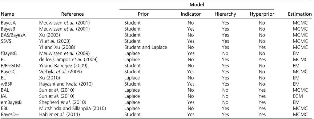
et al.2009; Yi and Banerjee 2009; Hayashi and Iwata 2010; Leeet al.2010; Shepherdet al.2010; Sun et al.2010; Xu 2010). A collection of the Bayesian methods used for phe-notype prediction and breeding value estimation is listed in Table 1 with some central features common to several of the methods.
While the proposed methods are competent and useful, wefind the recent development a bit disturbing for a couple of reasons. In thefirst place, rather than introducing a
tailor-Copyright © 2012 by the Genetics Society of America doi: 10.1534/genetics.112.139014
Manuscript received January 26, 2012; accepted for publication April 15, 2012 Supporting information is available online at http://www.genetics.org/content/ suppl/2012/05/02/genetics.112.139014.DC1.
1Corresponding author: Department of Agricultural Sciences, P.O. Box 28, Koetilantie
5, University of Helsinki, Helsinki FIN-00014, Finland. E-mail: [email protected].fi
made algorithm for every single model variant and empha-sizing the differences between the variants, it might be more helpful to try to focus on the similarities or on the common framework of the methods. The second concern of ours is the widespread fashion of mixing the model and the parameter estimation in a way that it is hard to follow what is the model, the likelihood, and the priors and what is the estimator. In this article our intention is to respond to the above-mentioned concerns by (1) carefully building a hierarchical Bayesian linear model and showing how many of the different models suggested in the literature can be seen as special cases of the more general one and (2) deriving a generalized EM algo-rithm for the parameter estimation in a way that presents explicitly how the model is translated into an algorithm.
In typical single-nucleotide polymorphism (SNP) data the number of markers is far greater than the number of indi-viduals, and hence in multilocus association models there usually are a lot more explanatory variables than observa-tions. This leads to a situation where some kind of selection of the predictors is required, either by discarding the un-important predictors or by shrinking their effects toward zero (e.g., O’Hara and Sillanpää 2009). Contrary to the fre-quentist way of deriving an estimator by adding a penalty to the loss function (e.g., penalized maximum likelihood, such as ridge regression and Lasso), in the Bayesian context the shrinkage-inducing mechanism is included into the model, namely by specifying an appropriate prior density for the regression coefficients. Although it is clearly more logical to consider the assumptions about the model sparseness as a part of the model (the prior is a part of the model) rather than a part of the estimator (a penalty is a part of the esti-mator), the difference may seem trivial in practice. However, the fact that in the Bayesian context the model includes all
available information permits the estimator to be always the same, either the whole posterior density or a maximum a posteriori(MAP) point estimate, and this enables the straight-forward translation of the model into an algorithm.
Model-wise our purpose is to examine the behavior of different submodels and prior densities, especially to com-pare the pros and cons of Student’stand Laplace priors. We want to explain the significance of the parameterization and hierarchical structure of the model for elegant derivation of posterior densities and mixing or convergence properties of an estimation algorithm and to emphasize in particular the beauty of the hierarchical specification of the prior density, contrary to the common enthusiasm to integrate out inter-mediate parameters when working within the EM context.
Estimation-wise we reclaim an approach familiar to those acquainted with MCMC, Gibbs sampling in particular, of deriving the fully conditional posterior density of every parameter and latent variable. Since the fully conditional posteriors are known distributions, we know the conditional posterior expectations and maximums required by the EM algorithm without integrating or setting the derivative to zero and solving, which is the traditional way to derive estimation steps in the EM framework. One of our purposes is to bring the MCMC and EM estimation frameworks closer together and, more generally, to point out that this approach makes it possible to construct an infinite variety of different algorithms, including EM algorithms, with differ-ent parameters considered as “missing data,” and type II maximum-likelihood algorithms, where all parameters are maximized (Tipping 2001), as well as mixtures of the pre-vious algorithms and Gibbs sampling, where some variables are stochastically sampled (stochastic EM) (e.g., Lee et al.
2008; Zhanet al.2011).
Table 1 Bayesian methods of phenotype prediction and breeding value estimation based on multilocus association models proposed in the literature
Model
Name Reference Prior Indicator Hierarchy Hyperprior Estimation
BayesA Meuwissenet al.(2001) Student No Yes No MCMC
BayesB Meuwissenet al.(2001) Student Yes Yes No MCMC
BAS/BayesA Xu (2003) Student No Yes No MCMC
SSVS Yiet al.(2003) Student Yes Yes No MCMC
Yi and Xu (2008) Student and Laplace No Yes Yes MCMC
fBayesB Meuwissenet al.(2009) Laplace Yes No No EM
BL de los Camposet al.(2009) Laplace No Yes Yes MCMC
R/BhGLM Yi and Banerjee (2009) Student No Yes No EM
BayesC Verbylaet al.(2009) Student Yes Yes No MCMC
BL Xu (2010) Laplace No Yes No EM
wBSR Hayashi and Iwata (2010) Student Yes Yes No EM
BAL Sunet al.(2010) Laplace No No Yes MCMC
IAL Sunet al.(2010) Laplace No No Yes ECM
emBayesB Shepherdet al.(2010) Laplace Yes No Yes EM
EBL Mutshinda and Sillanpää (2010) Laplace No Yes Yes MCMC
BayesDp Habieret al.(2011) Student Yes Yes Yes MCMC
Hierarchical Model
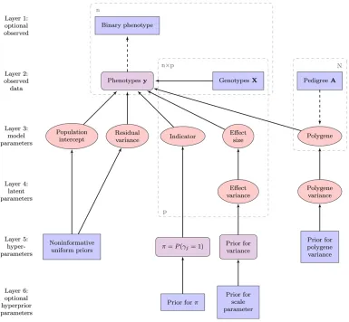
Our hierarchical model, depicted as a directed acyclic graph in Figure 1, has a total of six layers, two of which are op-tional. The observed data, located in layers 1 and 2 in the graph, comprises phenotype and genotype information, plus a known pedigree, of a sample of related individuals. The phenotype measurements of the nindividuals, denoted by ann-vectory, are assumed to be either continuous or binary; in the latter case the observed phenotypes are located in layer 1 in Figure 1. The genetic dataXare ann·pmatrix consisting of the genotypes ofpbiallelic SNP markers, coded as the number of the reference alleles, 0, 1, and 2, and stan-dardized to have zero mean and unity variance. The pedigree information is given in the form of an additive genetic rela-tionship matrix (Lange 1997), commonly denoted byA.
Linear model
The phenotypes are connected to the marker and pedigree information with a normal linear association model
y¼b01XGb1Zu1e; (1)
where b0 is the population intercept, and the n-vector e corresponds to the residuals, assumed normal and in-dependent, e Nnð0;Ins20Þ. If necessary, the intercept
b0can be easily replaced with a vector of environmental variables.
The second term on the right-hand side of the Equation 1 comprises the observed genotypesXand the allele substitution effectsGb, modeled following Kuo and Mallick (1998) as a prod-uct of the size of the effect and a variable indicating whether the marker is linked to the phenotype. In Equation 1,bis apvector of regression coefficients, denoting the additive effects sizes, and
G ¼diag(g)¼diag(g1,. . .,gp) is ap·pdiagonal matrix of
indicator variables, whosejth diagonal elementgjhas value 1 if
thejth SNP is included in the model and 0 otherwise.
The termuin Equation 1 denotes the additive polygenic effects due to the combined effect of an infinite number of loci. It represents the genetic variation not captured by the SNP markers, as well as takes account of residual dependen-cies between individuals (Yuet al.2006). The total number of individuals in the data is denoted by an uppercase N, in contrast to the lowercasenrepresenting the number of indi-viduals with an observed phenotype. The vector of polygenic effects,u¼[u1. . .uN]9, has anN-dimensional multivariate
normal prior distribution with mean vector0and covariance matrix As2
u, where A is the additive genetic relationship
matrix and s2
u is the additive variance of the polygenes. Z = [In|0n·N2n] is an n·N design matrix connecting the
polygenic effects to the observed phenotypes.
The individuals, or their phenotypic values yi, are
as-sumed conditionally independent given the genotype infor-mation Xand the polygenic effect u. This assumption and the described linear marker association model (1) give a multivariate normal likelihood Nnðb0þXGbþZu;Ins20Þ for the phenotype vectory, or, due to the independence of the observations the likelihood can be interpreted also as a univariate normal density N ðb0þ
Pp
j¼1gjbjxijþui;s20Þ for a single observationyi. The parameters of the multilocus
association model that are present in the likelihood function are located in the“parameter”level of the graph in Figure 1.
Shrinkage-inducing priors
A central feature of handling an oversaturated model is se-lection of the important predictors (e.g., O’Hara and Sillanpää 2009). In the Bayesian context the sparseness is included into the model by specifying such a prior density for the regres-sion coefficients that it represents thea prioriunderstanding that most of the predictors have only a negligible effect, while there are a few predictors with possibly large effect sizes. A prior that would evince this idea should consist of a probability mass centered near zero and a probability mass distributed over the nonzero values, including a reasonably high probability for large values. The most prominent prior densities used for acquiring the desired shape are Student’s
t(e.g., Meuwissenet al.2001; Xu 2003) and Laplace distri-butions (de los Campos et al. 2009), either alone or com-bined with a point mass at zero (Meuwissen et al. 2001; Shepherdet al.2010) or as a mixture of two Student’st dis-tributions with different variances (stochastic search vari-able selection) (e.g., Verbyla et al.2009). Student’st and Laplace densities possess several favorable features, includ-ing high kurtosis and proportionally heavy tails, that make them worthy candidates for shrinkage-inducing priors. How-ever, in some cases, especially with an oligogenic trait, the shrinkage introduced by these densities may not be suffi -cient and a mixture prior with a point mass at zero is re-quired to produce the optimal sparseness. Due to its weaker shrinking ability the Student’stprior is more prone to the problem than the Laplace prior. In fact, Pikkuhookana and Sillanpää (2009) and Hayashi and Iwata (2010) have noted that adding a point mass at zero to a Student’stprior model improves the performance, due to the elimination of the cumulative effect of a multitude of insignificant but nonzero marker effects. Although the Laplace prior generates more sparseness, there is evidence in support of the usefulness of the Laplace and point mass mixture prior (Shepherd et al.
2010). The Laplace prior leads to an estimate nearly identi-cal to the frequentist Lasso estimate (Tibshirani 1996) and is therefore commonly denoted as the Bayesian Lasso (Park and Casella 2008). However, contrary to the original fre-quentist version, the Bayesian Lasso shrinks the unimportant coefficients to small values instead of zero (Sunet al.2010), which also supports the putative benefit of a mixture prior. The insertion of a zero-point mass into the prior of the marker effects is carried out by adding an indicator variable
into the model to tell whether the effect of a given predictor variable comes from the density part (Laplace or Student’st) or from the point mass part of the prior, that is to say whether the variable is included into the model or not. Fol-lowing Kuo and Mallick (1998) the marker effects are mod-eled as a product of the indicator variablegjand the effect sizebj, which are considereda prioriindependent; hence the
joint prior of the marker effect becomes simplyp(gj,bj)¼ p(gj)p(bj), where p(gj) is a Bernoulli density with a prior
probability for a marker to be linked to the trait, the effect size priorp(bj) being either a Student’stor a Laplace density.
Both Student’s t and Laplace distribution can be expressed as a scale mixture of normal distributions with a common mean and effect-specific variances. The Student’s
t density can be formulated as a scale mixture of normal distributions with variances distributed as a scaled inverse
x2, while a Laplacian density can be presented in a similar manner, the mixing distribution now being an exponential one. As the hierarchical representation of the Student’s
tdistribution leads to conjugate priors for the normal likeli-hood parameters, it is a perfect choice for a conjugate anal-ysis. The exponential prior of the effect variancess2
j in the
Laplace model is not conjugate to the conditionally normally distributed effect sizes bjjs2j; however, the inverse of the
effect variance has an inverse Gaussian fully conditional distribution function (Chhikara and Folks 1989). Within the MCMC world, the hierarchical formulation of the prior densities, also known as model or parameter expansion, is a well-known device to simplify computations by transform-ing the prior into a conjugate and hence enabltransform-ing Gibbs sampling and to accelerate convergence of the sampler by adding more working parts and therefore more space for the random walk to move (see,e.g., Gilks et al.1996; Gelman 2004; Gelmanet al.2004). In MAP estimation, on the other hand, a commonly adopted approach to try to simplify the model is to integrate out the effect variances. However, the conjugacy maintained by preserving the intermediate vari-ance layer is a valuable feature also for a MAP estimation, as it enables the straightforward derivation of the fully condi-tional posterior density functions.
Hyperparameter selection in MAP estimation
next layer of the model hierarchy, and hence inevitably at one level or another of the hierarchy the user has to provide some values.
In Bayesian Lasso models the hyperparameters are usually treated as random parameters, while in Student’s
t-based models it is more common to hold them as con-stants, even though opposed examples exist; e.g., Xu (2010) proposes a Laplace model with constant hyperpara-meters, while Yi and Xu (2008) and Habier et al. (2011) estimate the hyperparameters of a Student’stmodel with an MCMC algorithm (see Table 1). However, there seems not to be a single work proposing an EM algorithm for hypeparameter estimation of a Student’s t model. On the contrary, Carbonetto and Stephens (2011) present a varia-tional Bayes MAP-estimation algorithm that swaps impor-tance sampling for those hyperparameters. The absence of examples in the literature corroborates our own experimen-tation (results not shown) that the hyperparameters of a Stu-dent’stmodel cannot be estimated with an EM algorithm, and therefore, since we are committed to proceed with EM estimation, we adopt the common fashion of including the optional hyperprior layer into the Laplace model, but exclude it from the Student’stmodel.
Since the tuning of the model will be harder the more parameters there are to adjust, it is reasonable to try to manage with as few as possible. To this end we have decided to hold the degrees of freedomnof the Student’st
prior constant and estimate or adjust only the scale param-eters of the prior densities (l2 is the inverse scale of the Laplace prior, whilet2is a scale parameter of the Student’s
t prior) along with the prior probability p that a SNP is linked to the trait. Provided that we do estimate the model parameters with an EM algorithm, it is anyway less impor-tant to determine the shape of the prior densities, since the only information that passes to the posterior is the expected or maximum value of the density. This is one of the key fea-tures under which sampling-based MCMC and optimization-based MAP estimation differ from each other: when the es-timate is generated by sampling from a posterior density, the shape of the prior density is of crucial importance since the posterior is formed as the product of the prior and likelihood functions, as is well known. However, in MAP estimation one needs to be more concerned about the behavior of the expected or maximum points of the product function than about the actual shape of the function. Even though the model itself is the same regardless of the estimation method, this difference in the behavior of the estimation algorithm has to be taken into account when specifying the hyperpara-meter values. Further, as noted in the previous paragraph, it seems that the different behavior of the algorithms may also favor different model structures.
Hyperparameter values
To optimize the behavior of the estimation algorithm, the pre-determined hyperparameters of the Student’stdistribution are selected in a way that the fully conditional posterior
expecta-tion of the effect variance,Eðs2
j j dataÞ ¼ ðb
2
j þnt2Þ=ðn21Þ,
is mainly determined by the the square of the effect sizebj. By
setting the degrees of freedomn¼2, the posterior expecta-tion will becomeb2j þ2t2, so if we choose a small value for
the scalet2, the estimate of the variance stays always pos-itive, but is shrunk toward zero strongly if bj is small
ðbj1 ⇒ b2j bjÞ while left intact when bj is large
ðbj1 ⇒ b2
j bjÞ. Since t2 is assumed to be somewhat
data specific and affect the results, its value requires tuning. Under the Laplace model we give the rate parameter
l2 of the exponential density a conjugate gamma hy-perprior. The conditional posterior expectation of l2 is
Eðl2jdataÞ ¼ ðkþpÞ=ðjþPs2
j=2Þ; since p is very large,
the impact oft2into the posterior expectation is negligible, and therefore the shape parameter k of the Gamma(k, j) density is set to one. The rate parameter jaffects the pos-terior expectation ofl2, and hence its value has to be tuned. The indicatorG¼diag(g) has a Bernoulli prior with a prior probabilityp¼P(gj¼1) for the SNPjcontributing to the trait.
The value given for the probabilitypalso represents our prior assumption of the proportion of the SNP markers that are linked to the trait. Loosely speaking, although the marker den-sity and the distance of markers to putative QTL have their effects, it is quite reasonable to say thatp is the number of SNP markers in the data divided by our prior assumption of the number of QTL affecting the trait. The probabilityp can be assumed either known or unknown, the latter approach inserting an additional layer to the hierarchical model (the
“prior forp”box of layer 6 in Figure 1). The indicator affects the shrinkage of the marker effects concurrent with the shrink-age generated by the Student’stor Laplace priors of the effect sizesbj, and therefore the value ofp affects the selection of
the hyperparameters of the Student’s tand Laplace priors. When the probabilitypis assumed known, as in our Student’s
tmodel, it has to be tuned simultaneously to the other hy-perparameters (t2in our case). Under the Laplace model the probabilitypis estimated with a conjugate beta prior, either uninformative uniform Beta(1, 1) or an informative Beta(a,b) density. The informative beta prior embodies oura priori as-sumed number of QTL by settingaas the number of markers assumed to be linked to trait (nqtl) andb as the number of markers not to be linked (i.e.,b¼p2nqtl,pbeing the number of markers). In the latter case the assumed number of QTL (nqtl) is the parameter to be tuned.
The population intercept b0 and the logarithm of the residual variance logs2
0 have uninformative uniform prior densities, sop(b0)}1 andpðs20Þ } 1=s20, which can be inter-preted as conjugateb0 N(0,N) ands20Inv-x2ð0; 0Þ pri-ors. The polygenic effect u has a multivariate normal prior distribution, with mean vector0and varianceAs2
u, where the
additive genetic relationship matrixAis a constant given by known pedigree, ands2u is the additive variance of the
poly-genes. The variance s2
u has an Inv-x2(2, 0.1) prior, whose
of each other. The prior independence of the indicator and the effect size, as suggested by Kuo and Mallick (1998), leads to the most straightforward parameterization of a mixture prior for the effects, which, in conjunction with the conjugacy ac-quired by the hierarchical formulation of the prior densities, enables an easy derivation of a closed-form fully conditional posterior distribution for every parameter and latent variable in the model. The fully conditional posterior densities are given in the Appendix, and the derivations of the densities are detailed inSupporting Information,File S1.
Binary response
In the case of a binary phenotype the above general linear model (1) is not valid. In a linear regression model, the expected value of the response variable equals the linear predictor,E(y)¼b0+XGb+Zuin model (1). The value range of the linear predictor is the whole real axis, while the expected value of a binary variablew, being also the prob-ability of the positive outcome,E(wi)¼P(wi¼1), has to lie
between zero and one. However, we can easily bypass the problem by introducing a continuous, normally distributed latent variabley, such that the binary variable
wi¼
1; when yi.0
0; when yi#0:
Now the latent variableyiis given by the model Equation 1
with a residualei N(0, 1), and hence the expected value
of the binary variable becomes
EðwiÞ ¼Pðwi¼1Þ ¼Pðyi.0Þ ¼FðEðyiÞÞ;
whereF() denotes the standard normal cumulative distribu-tion funcdistribu-tion, E(yi) being the linear predictor of model (1).
The probability of the binary variable, given the expected value of the latent variable, is Bernoulli with a success prob-abilityF(E(yi)). The latent variable parameterization of the
binary phenotype corresponds to a generalized linear model with the probit link function (Albert and Chib 1993).
The likelihood of the binary phenotype is the Bernoulli (F(E(yi))) distribution, while the normally distributed
re-sponse y is interpreted as a latent variable with a normal prior density given by the likelihood function corresponding the linear model in (1). Since the augmentation of the latent variable is an additional layer in the original hierarchical model (layer 1 in Figure 1), the other parameters (except the residual variance that has beenfixed to unity), and their fully conditional posterior densities, are the same as in the continuous-phenotype case.
Polygenic model
For a reference, we have considered a Bayesian version of G-BLUP, a classical animal model with a realized relation-ship matrix, where the genetic effects are assigned to individual animals, not to genetic markers,
y¼b0þZuþe; (2)
where u now represents the additive genetic values of the individuals. Genetic marker data can be incorporated into a traditional animal model in a form of a realized relationship matrix. A realized relationship matrix, commonly denoted by
G, estimated from the marker data, substitutes in the animal model the numerator relationship matrixA, estimated from the pedigree. We generated the genetic relationship matrix with the second method described in VanRaden (2008). Within the classical framework genomic breeding values are commonly estimated with known variance components, while in the Bayesian approach the variance components are estimated simultaneously with the genomic breeding values (Hallanderet al.2010). Contrary to the classical framework, the Bayesian inference is always based on variances that are estimated from data and hence are up-to-date and specific to the analyzed trait, letting also the uncertainty of the vari-ance components be incorporated into the breeding values. Even though,e.g., ASREML (Gilmouret al.2009) estimates the variance components from the data, and hence satisfies the up-to-date criterion, the variances are not estimated si-multaneously to the breeding values; instead, the preesti-mated variance components are considered constant while estimating the breeding values. The likelihood of the data under the animal model is simply multivariate normal with mean b0+Zu and covarianceIns20. Priors for the genetic valuesuand the population interceptb0are conjugate mul-tivariate normal NNð0;Gs2uÞ and uniform, respectively, G
being the genomic relationship matrix. The variances s2 0 and s2
u have inverse-x2 priors, uninformativepðs20Þ}1=s20, and aflat Inv-x2(2,M) with largeM, respectively. The latter differs from the prior density proposed for the additive ge-netic variance of the polygeneðs2
uÞof the multilocus
associ-ation model (1), since here the polygene has to cover all of the genetic variance, not only a small fraction, and hence the variance component needs to be able to get substantially higher values.
Parameter Estimation
Since we know the fully conditional posterior density of every parameter and latent variable, we could easily implement a Gibbs sampler to sample from those distributions. However, as the fully conditional posteriors are known distributions and hence the conditional expectations and maximums are known, we can just as easily use the distributions in implementing a fast algorithm of our choice to find a MAP estimate of the posterior density.
parameter vector to its expected value and the rest to its maximum-likelihood value, to conditional posterior expecta-tion and to condiexpecta-tional posterior maximum, respectively, in the Bayesian context. To enable handling of large marker sets the iterative updating in our algorithm is done one parameter at the time, conditionally on the other parameters remaining
fixed. This practice is a form of a generalized EM and can be seen as a further extension of the expectation-conditional-maximization (ECM) algorithm, as we update all of the pa-rameters individually, not only the ones to be maximized.
The partition of the variables into parameters and hidden variables is somewhat arbitrary, although often variances and other nuisance parameters are integrated out from the posterior by updating them into their conditional expectations. Under a Gaussian model the classification is even more vague, since the expected and the maximum values of the location parameters are the same (symmetric posterior density), and the corresponding values for the scale parameters with an inverse-x2posterior become equivalent by a slight modification of the prior hyperparameters. Thus, for it is not clear or even interesting which parameters are updated into their condi-tional maximums and which to condicondi-tional expectations, we base our method on an alternative description of the EM algo-rithm (Neal and Hinton 1999), regarding both of the steps as maximization procedures of the same objective function. Under the alternative description of the EM algorithm, the generalized expectation-maximization (GEM) algorithm corre-sponds to seeking to increase the objective function instead of attempting to maximize it. That is, we do not guarantee that the chosen arguments maximize the objective function, but know that the value of the function will increase with every update. The generalized algorithm has been proved to converge into same estimate as the standard EM algorithm, although possibly slower (Neal and Hinton 1999). A similar algorithm was imple-mented for the animal model (2).
GEM algorithm for a MAP estimate
1. Set initial values for parameter vectors. We use zeros for
b0, b, and u; small positive values, namely 0.1, for the variances; and 0.5 for the indicatorsg.
2. In the case of a binary phenotype, update the values of the latent variable y by replacing the current values yi
with the expected values of the truncated normal distri-butions (Equation A11),
yi:¼
8 > > < > > :
mi2 fðmiÞ
12FðmiÞ; when wi¼0
miþfFðmiÞ
ðmiÞ; when wi¼1;
wheremi¼b0þ Pp
j¼1gjbjxijþui;andf() andF()
de-note the standard normal density function and the dis-tribution function, respectively.
3. Maximize the posterior distributions ofb0andbj(for all j) by substituting the fully conditional expectations for
the current values of the parameters, one at the time. According to (A1) and (A2) we set
b0:¼1 n
Xn
i¼1 0 @yi2Xp
j¼1
gjbjxij2ui
1 A;
and
bj:¼
Pn i¼1
gjxij yi2b02 P
l6¼j
glblxil2ui
!
Pn
i¼1
gjxij
2
þs2 0 = s2j
:
4. Update the error variance s2
0 into its conditional expec-tation. Since the expected value of an Inv-x2(n,t2) dis-tribution isnt2/(n22), we get from (A3) the conditional expectation of the posterior distribution of s20 that sub-stitutes the existing value ofs2
0:
s2
0:¼
1
n22
Xn
i¼1 0
@yi 2 b02 Xp
j¼1
gjbjxij2ui
1 A 2
; for n.2:
5. Update the effect variancess2
j (for all j) to their
condi-tional expectations.
Under the Student’stprior model the fully conditional posterior distribution ofs2
j is an inverse-x2, as expressed
in (A4); hence we get
s2
j :¼
b2
j þnt2
n21 ¼b
2
j þ2t2; for n¼2:
The value set fort2has to be small to create the desired shrinking effect; the smaller the value is, the more shrinkage there will be. Under the Laplace prior model the precision, or inverse of the variance parameters s2
j,
has an inverse-Gaussian fully conditional posterior distri-bution (A5) and its expected value equals
s2 j :¼ bj ffiffiffi l p :
6. Replace the additive variance of the polygenes, s2
u, with
its conditional expectation, given by the Inv-x2 distribu-tion in (A6),
s2
u:¼
1
nuþN22
u9A21uþn
ut2u
¼1 N
u9A21uþ0:2
fornu¼2;t2u¼0:1, andN.2.
u:¼ Z9Zþs20 s2
u
A21 21
Z9ðy2b02XGbÞ:
8. Update the indicatorsgjone at the time. First compute
Rj¼pðyjgj¼1;⋆Þ pðyjgj¼0;⋆Þ
as expressed in (A8) and then substitute the fully condi-tional expectation for current values ofgj,
gj:¼Eðgjj⋆Þ ¼Pðgj¼1j⋆Þ ¼
pRj ð12pÞ þpRj:
9. If the hyperparameterslandpare estimated, update the values into conditional expectations. The expected value of a Gamma(k,j) density, the parameterjbeing inverse scale or rate, isk/j. Hence, from (A9) we get
l2:¼ ð1þpÞ 0 @jþX
p
j¼1 s2
j
2
1 A
21
for shape k¼1:
The expected value of a Beta(a,b) density isa/(a+b), so, from (A10),
p:¼ 1
2þp 0 @1þX
p
j¼1 gj
1
A for a¼b¼1;
and
p:¼ 1
2p 0 @aþX
p
j¼1 gj
1
A for b¼p2a;
where p is the number of SNP markers, and a can be considered as the number of segregating QTL (nqtl). The steps are repeated until convergence.
Example Analyses
In our example analyses we have considered the predictive performance and behavior of the model with the two alternative shrinkage priors, Student’stand Laplace, as well as the importance of the hierarchical formulation of the latter. Further, we have studied the necessity of the compo-nents of the model under the different prior densities. Therefore, in addition to the proposed model (1) we have considered a model without the polygenic component (i.e.,
u¼0), a model without the indicator variable (i.e.,g¼1), and a model lacking both of these components. We refer to these variants as I, II, III and IV, respectively. To examine the importance of the hierarchical definition of the Laplace prior for the model behavior we have implemented a nonhierar-chical variant of the Laplace prior model as our own GEM
version of the MCMC algorithm proposed by Hans (2009), with the prior density for the regression coefficientsbjbeing bj|lLaplace(0,l) and the hyperprior for the parameter lbeinglGamma(k,j) (note that here the hyperprior is assigned tolinstead ofl2). To compare the accuracy of the estimates given by the different models we have computed the genomic breeding values for the prediction set individuals and examined the Pearson’s correlation coefficient between the true and the estimated breeding values under the model vari-eties. The estimated breeding value GEBVi¼
Pp
j¼1xijgjbjþui
is simply the linear predictor of model (1). The possible bias of the estimated breeding value was measured with a regres-sion coefficient (cov(TBV, GEBV)/var(GEBV)) of the true breeding values on the estimated ones. In the absence of en-vironmental covariates, the heritability of the trait was esti-mated indirectly from the observed phenotypic variance and the estimate of the residual variance.
We have tested our method with two data sets, thefirst of which is simulated data introduced in the XII QTL-MAS Workshop 2008 (Lundet al.2009) and is freely available at the workshop homepage,http://www.computationalgenetics.
se/QTLMAS08/QTLMAS/DATA.html. We selected this
partic-ular data set to be used in our example analysis since the data have been used extensively in different studies (e.g., Usai
et al. 2009; Hallander et al. 2010; Shepherd et al. 2010), enabling an easy way to get some idea of the performance of our method in comparison to other methods proposed. The second data set is real pig (Sus scrofa) data, provided by the GENETICS journal to be used for benchmarking of genomic selection methods. The data have been described in detail by Clevelandet al.(2012).
Simulated data analysis
The XII QTL-MAS data set consists of 5865 individuals from seven generations of half-sib families, simulating a typical livestock breeding population (see Lund et al. 2009 for details). All of the individuals have information on 6000 biallelic SNP loci, evenly distributed over six chromosomes of length 100 cM each. Since SNPs with minor allele fre-quency ,0.05 within the learning set were discarded, the actual number of markers in the analysis was 5726. Thefirst four generations of the data, 4665 individuals, have both marker information and a phenotypic record and function as a learning set, while generationsfive to seven, 1200 indi-viduals, function as a prediction or a test set.
example analysis can therefore be examined directly by comparing the genetic values or true breeding values (TBV) and the genomic breeding value estimates (GEBV). Equally, the estimated effects and locations of the loci can be directly compared to the real ones.
The first set of analyses comprises estimation of the breeding values with all of the 13 above-mentioned model variants: 4 variants for all of the prior densities and the animal model (2) as a reference. The prior hyperparameters of the Student’stprior model were set tot2¼0.01 andp¼ 0.0052, the latter expressing a prior assumption of 30 seg-regating QTL (nqtl¼30). The Laplace models included the additional hyperprior layer, so the corresponding hyperpara-meters were estimated simultaneously to the model param-eters with hyperpriorsl2Gamma(1, 1) andpBeta(1, 1) for the hierarchical version andlGamma(1, 100) and
pBeta(30,p230) for the nonhierarchical version. In the animal model (2) the scale t2
u of the prior of the additive
genetic variance was set to 1600.
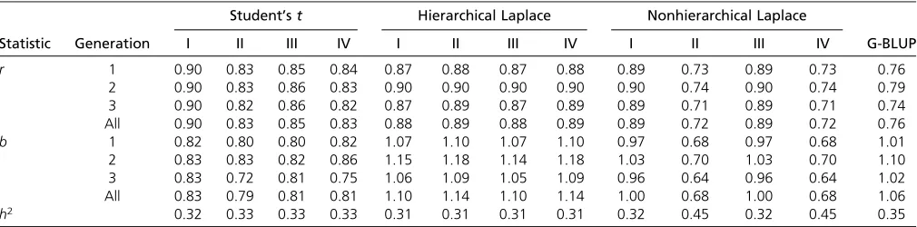
The results of the analyses, summarized in Table 2, sug-gest that the Student’stmodel benefits from the addition of a zero-point mass in the prior density, as the over all gen-erations correlation rbetween the true and the estimated breeding values increased from 0.83 to 0.90 when the in-dicator variable was included in the model (from 0.83 to 0.85 if there was no polygenic component in the model).
The hierarchical Laplace model seems to actually suffer from the addition of the indicator variable, as the correla-tions decreased slightly, from 0.89 to 0.88, if the indicator variable was present. The estimated proportion of markers contributing the phenotype, or the value ofp, in the hier-archical Laplace model was ’0.8, so the majority of the markers were considered linked to the trait. The estimated value of the parameterlwas’75 in all of the hierarchical model variants. Contrary to the hierarchical version, the nonhierarchical Laplace model requires the indicator vari-able. In this case the estimated proportion of contributing markers was ,2% (p ¼ 0.018). There was a striking im-provement in the performance of the nonhierarchical model
after the addition of the indicator variable: the value of the correlation coefficient grew from 0.72 to 0.89 and that of the regression coefficient from 0.68 to blank 1.00. The esti-mated value oflwas’37 under both the models with the indicator variable and ’44 under the models without an indicator.
The polygenic component u appears to be beneficial when the Student’stprior has been used with an indicator variable, but has no impact when the prior has been used without an indicator or with either of the Laplace priors. Since the heritability calculated from data in the QTL-MAS data set is 0.32, it seems that all of the models but the nonhierarchical Laplace model without an indicator are ca-pable of estimating it quite accurately. As expected, the results indicate superiority of the multilocus association model over the animal model. However, the Bayesian animal model with unknown variance components performed re-markably well when compared to a frequentist G-BLUP, the latter getting a correlation value of 0.75, when the cor-rect variance components were given.
Even though these results are based on only one data set and hence are special cases and also best-case scenarios in the sense that the prior hyperparameter values have been selected to yield best accuracy, they provide an important starting point for a comparison of the model performances by reproducing the procedure performed in the literature concerning this particular data set (e.g., Lundet al. 2009; Usai et al. 2009; Shepherd et al. 2010). The correlation values obtained by Usaiet al.(2009) for a G-BLUP model, a Student’stmodel without an indicator variable or a poly-gene, and a frequentist Laplace model without an indicator variable or a polygene are equal to our corresponding cor-relation values (0.75, 0.83, and 0.89, respectively). This is noteworthy, since their estimates are acquired by either MCMC simulation or a LARS algorithm, both requiring sev-eral hours of run time, while ours are acquired by an EM algorithm that takes only a few minutes. Shepherd et al.
(2010) observed a correlation value 0.88 under their non-hierarchical Laplace model with indicator variables, which is Table 2 QTL-MAS data
Student’st Hierarchical Laplace Nonhierarchical Laplace
Statistic Generation I II III IV I II III IV I II III IV G-BLUP
r 1 0.90 0.83 0.85 0.84 0.87 0.88 0.87 0.88 0.89 0.73 0.89 0.73 0.76
2 0.90 0.83 0.86 0.83 0.90 0.90 0.90 0.90 0.90 0.74 0.90 0.74 0.79
3 0.90 0.82 0.86 0.82 0.87 0.89 0.87 0.89 0.89 0.71 0.89 0.71 0.74
All 0.90 0.83 0.85 0.83 0.88 0.89 0.88 0.89 0.89 0.72 0.89 0.72 0.76
b 1 0.82 0.80 0.80 0.82 1.07 1.10 1.07 1.10 0.97 0.68 0.97 0.68 1.01
2 0.83 0.83 0.82 0.86 1.15 1.18 1.14 1.18 1.03 0.70 1.03 0.70 1.10
3 0.83 0.72 0.81 0.75 1.06 1.09 1.05 1.09 0.96 0.64 0.96 0.64 1.02
All 0.83 0.79 0.81 0.81 1.10 1.14 1.10 1.14 1.00 0.68 1.00 0.68 1.06
h2 0.32 0.33 0.33 0.33 0.31 0.31 0.31 0.31 0.32 0.45 0.32 0.45 0.35
Shown are correlation coefficients (r) between the estimated and true breeding values and regression coefficients (b) of the true breeding values on the estimated ones within single prediction set generations (generations 1–3) and in the whole prediction set (All), plus heritability estimates (h2), under different models in the QTL-MAS data set.
surprisingly slightly inferior to the correlation 0.89 we obtained with our corresponding model.
The breeding value estimates produced by the Student’st
model tended to be biased downward (regression coefficient
b ’ 0.8), while the hierarchical Laplace model produced slightly upward-biased values (b ¼ 1.1 with an indicator and 1.4 without one). The most unbiased values were obtained with the nonhierarchical Laplace model with an indicator variable and with the Bayesian G-BLUP (b ¼
1.00 and 1.06, respectively). The breeding values acquired by the frequentist G-BLUP, with the correct variance compo-nents, are biased downward withb¼0.88. Since the bias of the estimated breeding values is important mainly when comparing breeding values estimated with different meth-ods, which is not advised in any case, we do not concentrate on the bias of the estimates in our subsequent analyses of the data replicates.
Simulated data replicates
To further examine the model performance in a less data-specific situation, with the influence of sampling variation diminished, we generated 99 replicates of the QTL-MAS data set of approximately the same heritability to have a total of 100 phenotype sets (99 plus the original one). The phenotypic value of a given individual in the QTL-MAS data being the sum of the genetic value of that individual and a random residual (Lundet al.2009), the replicated pheno-types were obtained by simply resampling the residuals from a normal density N(0, var(TBV)(1/h2 2 1)), where var (TBV) denotes the observed variance of the genetic values and the heritability h2 ¼0.3. The 100 replicated data sets were analyzed with the most promising and/or interesting model variants.
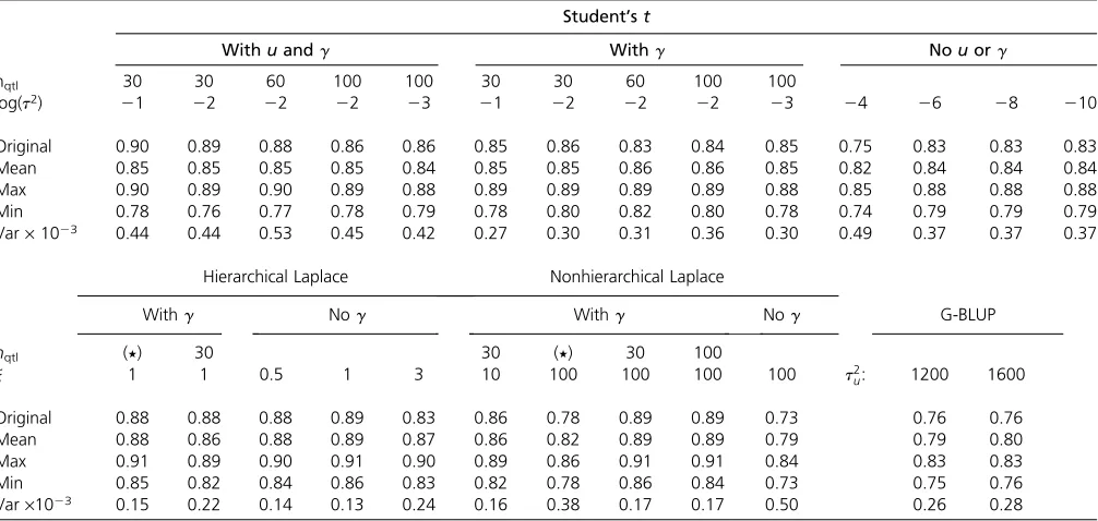
The Student’stmodel with both indicator and polygenic components (variant I) was the most accurate model variant in the preliminary analysis and hence was selected as a mat-ter of course for closer inspection. As the prior hyperpara-meters t2 and p of the Student’s t model are given, one objective is to consider the potential influence of the se-lected hyperparameters on the predictive performance of the model. We therefore carried out an analysis with five different parameter combinations; the results of the analy-ses, shown in Table 3, comprise the correlation between the true and genomic breeding values within the prediction set individuals in the original QTL-MAS data, in addition to the mean, maximum, minimum, and variance of the correlation in the set of 100 analyses.
The parameter combinations comprise three values for the number of QTL, namely 30, 60, and 100, in addition to three values covering three orders of magnitude from 1021 to 1023, for the scale parametert2. Even though the corre-lation observed within the original data set varies between 0.86 and 0.90 depending on the hyperparameter values, the range of the mean values is much less wide, only from 0.84 to 0.85. Also the maximum and minimum values show less variation between different priors. To examine the effect of
the polygenic component, the Student’s t model with an indicator, but the polygene u set to zero (variant III), was tested with the same parameter combinations as the model including both of the components. On average the impact of the polygene in the replicated data sets is less clear than in the individual original QTL-MAS data, even though the highest of the observed correlations were slightly larger when the polygene was included into the model, 0.90 and 0.89, respectively, and the means of the correlations were actually lower in the polygene model, 0.85 and 0.86, respec-tively (Table 3). Corresponding to the observations with the polygene model, the mean and maximum values of the cor-relations were not influenced by the selection of the hyper-parameters, contrary to the correlation within the original QTL-MAS data set. The Student’stmodel without an indi-cator or a polygenic component (variant IV) was tested by analyzing the replicated data sets with four alternative val-ues for the scale parameter t2, covering seven orders of magnitude from 1024to 10210. Since here the Student’st prior alone has to provide the shrinkage of the marker effects, the values given for the scale parametert2are sub-stantially smaller than in the indicator model, leading to more intensive shrinkage. This model was the least sensitive to the hyperparameter values, as all of the observed corre-lations are the same while the hyperparameter t2 varies between 1026 and 10210. On average, the performance of the three models was less divergent than it appeared to be after the analysis of the single original data set, the highest mean correlations ranging between 0.84 and 0.86 and max-imums between 0.88 and 0.90, in contrast to the correspond-ing values in the original data analysis, rangcorrespond-ing between 0.83 and 0.90.
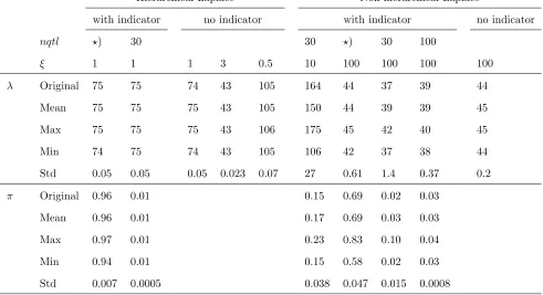
3, the best correlation was acquired under the hierarchical Laplace model without an indicator, with a Gamma(1, 1) prior for l2, where the maximum correlation exceeded 0.91, while the mean correlation was 0.89. The model with indicator remained slightly inferior, as suggested by the pre-liminary analysis, the mean correlation being 0.88 with a uniform prior forp. The estimated values of the parameter
l varied only slightly within the 100 analyses and were
’105, 74, and 43 with hyperprior rates 0.5, 1, and 3, re-spectively (seeTable S1). The estimates of the probabilityp were near 1 under the Beta(1, 1) prior and’0.01 under the Beta(30,p230) prior. The informative prior forpdistracted the model quite badly, resulting in the mean correlation dropping from 0.89 (no indicator) to 0.86 (informative prior for indicator). Under the nonhierarchical Laplace model a Gamma(1, 100) prior for the parameterlwith a Beta(30,
p 2 30) prior for the indicator probabilityp were the best choices, leading to correlation values equal to the best ones from the hierarchical Laplace model. The model seems to be quite robust regarding to the indicator prior, as the prior assumption of 30 or 100 segregating QTL led to almost sim-ilar results.
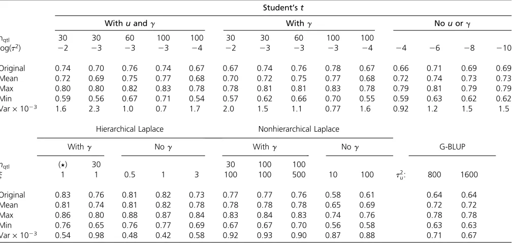
Binary data
The binary phenotype model was tested by using the replicates of the QTL-MAS data with dichotomized pheno-typic values. A binary phenotype was acquired by simply cutting the data in two in a way that 80% of the learning set
individuals get a binary value 0 and 20% get a binary value 1. The selection of the success probability 0.2 was arbitrary, except that we wanted to avoid the extreme variance values 0.25 and 0 for the Bernoulli response variable, with corresponding success probabilities 0.5 and 0 (or 1).
The results for the Student’s t model, for both of the Laplace models and for the Bayesian G-BLUP are presented in Table 4. The results show that the hierarchical Laplace model suffers less from the reduced information of the data than the nonhierarchical Laplace model and the Student’s
tmodel.
The mean correlations acquired by the nonhierarchical Laplace models and the best Student’s t models are only 0.78 and 0.77, respectively, while the best mean correlation observed under the hierarchical Laplace model is 0.82. The best-performing Student’stmodels are the models with an indicator, with hyperparametersp¼100/pandt2¼1023, while the presence of the polygenic component seems to be of no importance. The nonhierarchical Laplace model per-formed again poorly without the indicator variable, while the hierarchical model performed better without one. The estimated parameter values under the hierarchical Laplace model were the same as in the continuous phenotype case:
l = 105, 74, and 43 with hyperprior rates 0.5, 1, and 3, respectively, andpeither’1 or 0.1, depending on the prior. Under the nonhierarchical Laplace model l ¼470 (model variant IV, no indicator), 44 (with indicator, 49 when no indicator was present), and 11 (with indicator) with Table 3 Data replicates
Student’st
Withuandg Withg Nouorg
nqtl 30 30 60 100 100 30 30 60 100 100
log(t2) 21 22 22 22 23 21 22 22 22 23 24 26 28 210
Original 0.90 0.89 0.88 0.86 0.86 0.85 0.86 0.83 0.84 0.85 0.75 0.83 0.83 0.83
Mean 0.85 0.85 0.85 0.85 0.84 0.85 0.85 0.86 0.86 0.85 0.82 0.84 0.84 0.84
Max 0.90 0.89 0.90 0.89 0.88 0.89 0.89 0.89 0.89 0.88 0.85 0.88 0.88 0.88
Min 0.78 0.76 0.77 0.78 0.79 0.78 0.80 0.82 0.80 0.78 0.74 0.79 0.79 0.79
Var·1023 0.44 0.44 0.53 0.45 0.42 0.27 0.30 0.31 0.36 0.30 0.49 0.37 0.37 0.37
Hierarchical Laplace Nonhierarchical Laplace
Withg Nog Withg Nog G-BLUP
nqtl (⋆) 30 30 (⋆) 30 100
j 1 1 0.5 1 3 10 100 100 100 100 t2
u: 1200 1600
Original 0.88 0.88 0.88 0.89 0.83 0.86 0.78 0.89 0.89 0.73 0.76 0.76
Mean 0.88 0.86 0.88 0.89 0.87 0.86 0.82 0.89 0.89 0.79 0.79 0.80
Max 0.91 0.89 0.90 0.91 0.90 0.89 0.86 0.91 0.91 0.84 0.83 0.83
Min 0.85 0.82 0.84 0.86 0.83 0.82 0.78 0.86 0.84 0.73 0.75 0.76
Var·1023 0.15 0.22 0.14 0.13 0.24 0.16 0.38 0.17 0.17 0.50 0.26 0.28
Shown is the correlation between the true and estimated genomic breeding values in the original QTL-MAS data, in addition to the mean, maximum, minimum, and variance of the correlation in the analyses of the 100 replicated data sets.nqtldenotes different hyperparameter values for the indicator under the Student’stmodel and different hyperprior parameter values for thepBeta(nqtl,p2nqtl) prior of the indicator under the Laplace models. (⋆) denotes the optional Beta(1, 1) prior of the indicator. Hyperparameter log(t2) is the logarithm of the scale of marker variance under the Student’stmodel, andjdenotes alternative hyperprior parameter values for the prior of
the rate parameterl2Gamma(1,j) under the hierarchical Laplace model andlGamma(1,j) under the nonhierarchical Laplace model. G-BLUP refers to the Bayesian
animal model (2) with a scale hyperparametert2
hyperprior rates 10, 100, and 500, respectively, and p ¼ 0.005 and 0.007 withnqtl¼30 and 100, respectively.
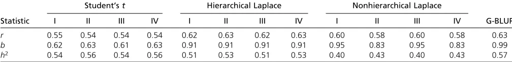
Real data analysis
The real pig data set consists of 3534 animals from a single pig line with genotypes from a 60k SNP chip and a pedigree including the parents and the grandparents of the geno-typed animals (Clevelandet al.2012). A total of 3184 gen-otyped individuals have a phenotypic record for a trait with predetermined heritability 0.62. As only the SNP markers with minimum allele frequency .0.05 were accepted to our analysis, the number of markers in the analysis was 45,317. The data set was analyzed with all of the 13 model variants.
The analysis of this data set provides a challenge concern-ing the proportion of SNPs to individuals. There is an upper limit to the number of effects with respect to the sample size, and even though the limit depends on the sample size (smaller data sets seem to be able to be more oversaturated) and the genetic architecture of the trait (a data set with an oligogenic trait may be less sensitive to oversaturation than one with a polygenic trait), Hoti and Sillanpää (2006) have suggested a limit of 10 times more predictors than individuals. We have reduced the number of markers in the multilocus as-sociation model by applying the sure independence screen-ing method of Fan and Lv (2008) for ultrahigh-dimensional feature space. The method is based on ranking the predictors with respect to their marginal correlation with the response variable and selecting either a predetermined proportion of
the predictors or the predictors exceeding a predetermined importance measure. We have chosen to take 10,000 best-ranking SNPs to the multilocus association study.
Contrary to the simulated data set, there are neither true genetic values of the individuals nor true effects of the QTL available, and hence we estimate the accuracy of the predicted breeding value by dividing the correlation between the GEBVs and the phenotypic values by the square root of the heritability of the trait. Since the data do not consist of a separate validation population, we compute the result statistics using cross-validation, where the 3184 individuals are randomly partitioned into 10 subsets (10-fold cross-validation) of 318 or 319 individuals.
The selection of the model hyperparameters is done similarly to that in the previous analyses, the only difference being the method of accuracy estimation. As previously, we tried quite a few values and selected the ones producing the best accuracy. Since here we do not have any extra in-formation but the pheno- and genotypes of the individuals, the procedure qualifies as a genuine parameter selection by cross-validation. The selected hyperparameter values under the Student’stmodel variants with the indicator (I and III) weret2¼1 andp¼0.05 andt2¼0.01 under the variants without an indicator (II and IV). The best hyperpriors for the hierarchical Laplace model werel2Gamma(1, 4000) for all variants (I–IV) andpBeta(1, 1) for the indicator (var-iants II and IV). For the nonhierarchical Laplace model the corresponding hyperpriors werelGamma(1, 4000) and
p Beta(1000,p21000) under the model variants with Table 4 Binary data
Student’st
Withuandg Withg Nouorg
nqtl 30 30 60 100 100 30 30 60 100 100
log(t2) 22 23 23 23 24 22 23 23 23 24 24 26 28 210
Original 0.74 0.70 0.76 0.74 0.67 0.67 0.74 0.76 0.78 0.67 0.66 0.71 0.69 0.69
Mean 0.72 0.69 0.75 0.77 0.68 0.70 0.72 0.75 0.77 0.68 0.72 0.74 0.73 0.73
Max 0.80 0.80 0.82 0.83 0.78 0.78 0.81 0.81 0.83 0.78 0.79 0.81 0.79 0.79
Min 0.59 0.56 0.67 0.71 0.54 0.57 0.62 0.66 0.70 0.55 0.59 0.63 0.62 0.62
Var·1023 1.6 2.3 1.0 0.7 1.7 2.0 1.5 1.1 0.77 1.6 0.92 1.2 1.5 1.5
Hierarchical Laplace Nonhierarchical Laplace
Withg Nog Withg Nog G-BLUP
nqtl (⋆) 30 30 100 100
j 1 1 0.5 1 3 100 100 500 10 100 t2
u: 800 1600
Original 0.83 0.76 0.81 0.82 0.73 0.77 0.77 0.76 0.58 0.61 0.64 0.64
Mean 0.81 0.74 0.81 0.82 0.78 0.78 0.78 0.78 0.65 0.69 0.72 0.72
Max 0.86 0.80 0.88 0.87 0.84 0.83 0.84 0.83 0.74 0.76 0.78 0.78
Min 0.76 0.65 0.76 0.77 0.69 0.67 0.67 0.70 0.56 0.58 0.63 0.63
Var·1023 0.54 0.98 0.48 0.42 0.58 0.92 0.93 0.90 0.87 0.88 0.71 0.67
Shown is correlation between the true and estimated genomic breeding values in the original but dichotomized QTL-MAS data, in addition to the mean, maximum, minimum, and variance of the correlation in the analyses of the 100 replicated and dichotomized data sets.nqtldenotes different hyperparameter values for the indicator under the Student’stmodel and different hyperprior parameter values for thepBeta(nqtl,p2nqtl) prior of the indicator under the Laplace models. (⋆) denotes the optional Beta(1, 1) prior of the indicator. Hyperparameter log(t2) is the logarithm of the scale of marker variance under the Student’stmodel, andjdenotes
alternative hyperprior parameter values for the prior of the rate parameterl2Gamma(1,j) under the hierarchical Laplace model andlGamma(1,j) under the
nonhierarchical Laplace model. G-BLUP refers to the Bayesian animal model (2) with a scale hyperparametert2
the indicator (I and III) andlGamma(1, 2000) under the variants without an indicator (II and IV). In all of the models including a polygenic component the prior for the polygenic variance was inverse-x2(2, 1). In the animal model (2) the scalet2
u of the prior of the additive genetic variance was set
to 1.3 · 106. Some of the hyperparameter and hyperprior parameter values are remarkably large due to the large var-iance of the phenotype, the varvar-iance being3500 (Cleveland
et al.2012). The accuracy estimates acquired with these hy-perparameters are presented in Table 5.
Contrary to the QTL-MAS data set, the phenotypes of the pig data are highly polygenic. The polygenic nature of the data is reflected by the select values of thea prioriassumed number of QTL (500 or 1000), as well as the relatively high accuracy of the Bayesian G-BLUP (correlation 0.63 with both Bayesian G-BLUP and the best of the association models, Table 5). Again, the Bayesian version of G-BLUP with simul-taneously estimated variance components was slightly more accurate than the frequentist version with predetermined heritability; the correlation and regression coefficients ac-quired by the frequentist method were 0.62 and 0.84, re-spectively. With the polygenic data the additional indicator variable (model variants I and III) was not as important as with the oligogenic QTL-MAS data. In fact, the accuracy of the Student’stmodel was the same (0.54) regardless of the indicator, while the nonhierarchical Laplace model was only slightly more accurate when the indicator was present (cor-relation 0.60 with and 0.58 without the indicator). Respec-tively, the hierarchical Laplace model suffered less from the addition of the indicator variable; the accuracy dropped from 0.63 only to 0.62 when the indicator was added. In this set of analyses the Student’stmodel performed remark-ably badly compared to the Laplace models. The best corre-lation obtained under the Student’stmodel was 0.55, while the hierarchical Laplace model came up to correlation 0.63. The hierarchical Laplace model was superior to the nonhi-erarchical model; the best observed correlations under the two models were 0.63 and 0.60, respectively. The estimated value of the hyperparameter l was 1.56 with all of the hierarchical Laplace model variants, 1.97 with the nonhier-archical variants with an indicator (I and III), and 4.68 with the nonhierarchical variants without an indicator (II and IV). The estimate for the indicator hyperparameter p had value 1 under the hierarchical Laplace model, reflecting the
redundancy of the indicator in the hierarchical model ver-sion, and was 0.11 under the nonhierarchical model. The polygenic component (model variants I and II) did not im-prove the model performance, probably due to the large number of markers.
In all analyses the algorithm was iterated until conver-gence was ascertained by the visualized behavior of the estimate values. The estimates converged rapidly, after only 20 GEM iterations when estimating the parameters of the Student’stmodel or the Laplace model without an indicator and after 13 or 14 GEM iterations when estimating the an-imal model parameters. The time needed varied from 12 sec to few minutes, depending on the model, the polygene being the slowest component to update. The only parameter re-quiring a substantial time to converge was the probability of a marker to be linked to the trait, p, of the hierarchical Laplace model. This hyperparameter tended to converge to a value near unity [with Beta(1, 1) prior] when given enough time, usually.200 GEM iterations. The GEM algo-rithm was implemented with Matlab version 7.10.0 (R2010a); the Matlab codes for the parameter estimation and the data replication are provided inFile S2. The analy-ses were performed with a 64-bit Windows 7 desktop com-puter with 3.50 GHz Intel(i7) CPU and 16.0 GB RAM.
Discussion
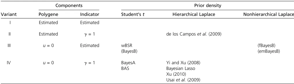
As declared in the Introduction, the purpose of this article is to (1)find a common denominator for many of the Bayesian multilocus association methods with shrinkage-inducing priors proposed in the literature and build a general model framework explaining the similarities and differences be-tween the proposed models and (2) examine the submodels especially regarding (a) different shrinkage prior densities, namely Student’stand Laplace; (b) possible advantage of the hierarchical formulation of the prior density for the model performance; and (c) the necessity of the model compo-nents, indicator variable, polygenic component, and hyperp-rior layer, under the different phyperp-rior densities.
Many of the 12 variants of the multilocus association model considered in the example analysis correspond closely to various methods proposed in the literature. As presented in Table 6, the variant IV Student’stmodel without a polygene (i.e., u =0) or an indicator (i.e., g ¼ 1) evidently equals Table 5 Pig data
Student’st Hierarchical Laplace Nonhierarchical Laplace
Statistic I II III IV I II III IV I II III IV G-BLUP
r 0.55 0.54 0.54 0.54 0.62 0.63 0.62 0.63 0.60 0.58 0.60 0.58 0.63
b 0.62 0.63 0.61 0.63 0.91 0.91 0.91 0.91 0.95 0.83 0.95 0.83 0.99
h2 0.54 0.56 0.54 0.56 0.51 0.53 0.51 0.53 0.40 0.43 0.40 0.43 0.57
Shown are breeding value accuracy and bias estimates from the real data analysis under the different model variants. Accuracy is determined as the correlation (r) between the estimated genomic breeding values and the phenotypic values, divided by the square root of the predetermined heritability, and the bias is determined as the regression coefficient (b) of the phenotypic values on the estimated genomic breeding values. Heritability (h2) estimates are calculated from estimated residual variance. G-BLUP refers to
BayesA (Meuwissenet al.2001; Xu 2003), while the variant III Student’stmodel with an indicator variablegbut without a polygene (u¼0) equals the weighted Bayesian shrinkage regression method (wBSR) proposed by Hayashi and Iwata (2010). Although the latter leads to the same marginal pos-terior for the marker effects as BayesB (Meuwissen et al.
2001; see Habieret al.2007 and Knürret al.2011 for com-ments), the two models have different hierarchical structures. In our model the marker effect sizebisa prioriindependent from the indicator g, and the marker effect is given as the productGb, as illustrated in Figure 2A. In the original BayesB the marker effect is given by b alone, since the likelihood does not include the indicator; instead, the indicator effect is through the effect variances2(see Figure 2B). The param-eterization of BayesB has been criticized by Gianola et al.
(2009). It is noteworthy that with our parameterization a MCMC algorithm for the model variant III would consist only of Gibbs steps, while with the original parameterization of BayesB Metropolis–Hastings steps are needed. Hence, even though we do not have direct evidence of the benefit of our parameterization to the GEBV accuracy, estimation-wise the advantage of this model structure is clear.
As noted in the Table 6, the variant IV hierarchical Lap-lace model without an indicator or polygene, with an esti-mated parameter l, covers several Bayesian Lasso models introduced by Yi and Xu (2008). A corresponding hierarchi-cal Laplace model with a prespecified hyperparameter has also been studied (Usai et al. 2009; Xu 2010). The fast versions of BayesB, fBayesB (Meuwissen et al. 2009) and emBayesB (Shepherd et al. 2010), correspond closely to the nonhierarchical Laplace model we have considered; however, again the structures are different. The structure of our nonhierarchical Laplace model is consistent with its hierarchical counterpart as only the latent variable layer is integrated out (see Figure 2C). The hierarchical structure of emBayesB is somewhat cryptic, since the indicator variable should work only through the marker effect but instead seems to be present also in the likelihood (Figure 2D). This
may explain the difference in the performances of the two models noted in the previous section. Further, unlike Shepherd
et al.(2010), we had no observation of the starting values of the algorithm affecting the result.
Our example analyses demonstrate that the Bayesian multilocus association model is a powerful tool to estimate the effects of genetic markers associated with QTL, leading to accurate breeding value estimates for genomic selection. Compared to the animal model, the multilocus association model benefits from the ability to assign effects of different magnitude for the different marker loci, which is especially important when the trait in question is oligogenic, as is the case in the QTL-MAS data set. In a more polygenic situation, however, the animal model is a competitive alternative, as can be seen in the pig data analyses. We have tested the two most prominent prior densities, Student’stand Laplace, for the marker effect sizes. Both of the densities work nicely as shrinkage priors; however, it seems that with a polygenic trait the Laplace prior is clearly more efficient. This is an important discovery, since the critique of marker association models and their bad behavior in a polygenic situation (e.g., Daetwyleret al.2010; Clarket al.2011) is mainly based on the observations on BayesB, that is, a Student’stmodel.
An EM algorithm for the Laplace model might be more easily tuned than an algorithm for the Student’st model, probably due to the additional hyperprior layer. The preva-lent approach, one that we have also adopted, is to treat the hyperparameters nandt2of the Student’stprior as given, while the hyperparameterlof the Laplace prior is treated as random. We do not know why others have chosen this course and why Carbonetto and Stephens (2011) use importance sampling for Student’stmodel hyperparameters within their otherwise optimization-based algorithm, but our reason is the old-fashioned trial and error: the alternative method did not work. We tried several priors for the scale parametert2of the effect variance in the Student’stmodel, but none of them led to a reasonable estimate (results not shown). Yi and Xu (2008) managed to estimate the hyperparameters of the Table 6 The 12 different submodels considered in the example analysis and the models proposed in the literature corresponding to the submodels
Components Prior density
Variant Polygene Indicator Student’st Hierarchical Laplace Nonhierarchical Laplace
I Estimated Estimated
II Estimated g= 1 de los Camposet al.(2009)
III u= 0 Estimated wBSR (fBayesB)
(BayesB) (emBayesB)
IV u= 0 g= 1 BayesA Yi and Xu (2008)
BAS Bayesian Lasso
Xu (2010) Usaiet al.(2009)
Student’stprior in a model without an indicator variable with uniform hyperprior densities by MCMC. However, the EM algorithm is less flexible in a sense that the variance of the fully conditional posterior density does not have an impact when a parameter is updated to its fully conditional posterior mean or maximum, contrary to MCMC sampling, where a large posterior variance gives great room for maneuver for the parameter to be updated. It appeared to be impossible to select such a prior density that neither the hyperpara-meters nor the effect variances would determine completely the posterior expectation. Gelman et al.(2004) advise aug-menting the model with an additional parameter breaking the dependence between t2 and s2
j, which should help
a Gibbs sampler not to get stuck, but even this method did not help the EM algorithm. The EM estimation of the prior
probability of a marker to be linked to the phenotype, p, proved also impossible with our hierarchical model. With any reasonable uninformative hyperprior the estimated value was almost unity, and the only way to obtain something smaller is to propose a highly informative hyperprior, one so informative that it kind of spoils the whole idea of estimat-ing the value. Therefore, the most reasonable approach seems to be to treat the hyperparameterst2andpof the Student’st prior model as given and determine the best ones, e.g., by cross-validation.
As mentioned earlier, although the hyperparameterlof the Laplace distribution was estimated from the data, the need for tuning of parameters passes to the next layer of the model hierarchy. This is clearly illustrated by proposing sev-eral gamma hyperpriors for the parameter and finding out Figure 2 Different hierarchical structures of models. (A) The hi-erarchical structure of our model, the effect size, and the indicator are independent and both con-tribute to the likelihood. (B) The hierarchical structure of BayesB (Meuwissenet al.2001). The in-dicator works through the effect variance. (C) The structure of the nonhierarchical Laplace model, the effect size and the indicator are independent and both con-tribute to the likelihood that there is no latent variable level. (D) The hierarchical structure of emBayesB (Shepherd et al.