On the Pleiotropic Structure of the Genotype–Phenotype Map and the Evolvability of Complex Organisms

(1)

INVESTIGATION

On the Pleiotropic Structure of the Genotype

–

Phenotype Map and the Evolvability

of Complex Organisms

William G. Hill1_{and Xu-Sheng Zhang}2 Institute of Evolutionary Biology, School of Biological Sciences, University of Edinburgh, Edinburgh, EH9 3JT, United Kingdom

ABSTRACTAnalyses of effects of mutants on many traits have enabled estimates to be obtained of the magnitude of pleiotropy, and in reviews of such data others have concluded that the degree of pleiotropy is highly restricted, with implications on the evolvability of complex organisms. We show that these conclusions are highly dependent on statistical assumptions, for example signiﬁcance levels. We analyze models with pleiotropic effects on all traits at all loci but by variable amounts, considering distributions of numbers of traits declared signiﬁcant, overall pleiotropic effects, and extent of apparent modularity of effects. We demonstrate that these highly pleiotropic models can give results similar to those obtained in analyses of experimental data and that conclusions on limits to evolvability through pleiotropy are not robust.

B

IOLOGICAL organisms are complex structures, so it is not surprising that their genes often show pleiotropic effects over two or more traits. Evidence comes both from observations on substitutions at individual loci and from genetic correlations among the traits at a population level. One view is that all genes are fully pleiotropic, at least at the quantitative level, in view of the highly interdependent and interactive nature of biological systems. Another view is that such an argument is irrelevant to genetic understanding, analysis, and application in that most loci are likely to affect no more than a small minority of traits in any biologically signiﬁcant way (Stearns 2010).

The general degree of pleiotropy is important in several areas, for example in understanding pathways of gene action, in assessing potential side effects of genetic manip-ulation of particular pathways, in assessing the impacts of selective genetic improvement programs, and in considering the opportunities for evolutionary change through new mutations that may induce both favorable and unfavorable effects onﬁtness.

In a recent perspectives paper Wagner and Zhang (2011) discuss the magnitude of pleiotropy for complex or quanti-tative traits. They argue that it is highly restricted, i.e., rather few traits are influenced by each gene, and conse-quently conclude there is more opportunity for evolutionary change according to Fisher’s (1930) geometric model than suggested by the analyses of Orr (2000) and for finding drugs specific for a particular genetic disease.

Different kinds of data sets were used by Wagner and Zhang, many of them collected by them and their col-leagues. One is based on mapping QTL using F2crosses of

selected lines of mice (Wagneret al.2008), but pleiotropy and linkage of nonpleiotropic QTL cannot readily be disen-tangled. The other is based on single mutant lines where this complication does not arise. Wang et al. (2010) analyzed four published data sets on mutants, two of which were very large: One included 253 morphological traits, each recorded on 2449 haploid lines ofSaccharomyces cerevisiae, each mu-tant for a different gene. The mean number of traits affected by each line was 21.6 and the median, 7, was smaller be-cause the distribution of the number per line was of expo-nential form. In the other data set, for 4905 genes and 308 traits in mice, the mean was 8.2 and the median 6. Overall a signiﬁcant degree of pleiotropy was found for no more than 10% of traits observed.

doi: 10.1534/genetics.111.135681

Manuscript received October 10, 2011; accepted for publication December 24, 2011 1_{Corresponding author: Institute of Evolutionary Biology, University of Edinburgh, West}

Mains Rd., Edinburgh, EH9 3JT, United Kingdom. E-mail: [email protected] 2_{Present address: Statistics, Modelling, and Bioinformatics, Centre for Infections,}

(2)

They computed the Euclidean distance, a measure of the total of individual trait effects detected to be signiﬁcant for that gene, and found that it increased more rapidly than would be expected if there were no relation between overall gene effects and number of traits affected (Wanget al.2010, Box 4).

Their third conclusion was that there was strong modu-larity of effects,i.e., that genes differed in the suite of traits they affected. The association between genes and traits was represented by a bipartite network and the presence of a modular structure detected by methods developed in phys-ics (Barber 2007). A series of random networks was gener-ated having the same marginal properties, i.e., numbers of traits detected for each gene and correspondingly genes af-fecting each trait, and the association of genes and traits was found not to be randomly distributed.

Other data that indicate substantial pleiotropy have, however, been published (Stearns 2010). For example, many studies have been undertaken in Drosophila mela-nogasterby Mackay and colleagues. Of theP-element muta-tions they screened, 22% affected abdominal bristle number, 23% sternopleural bristle number, 41% starvation stress re-sistance, 5.6% olfactory behavior, 22% wing shape, 37% locomotor startle response, and 35% aggressive behavior (Mackay 2010). Thus many genes affect each trait and each gene affects many traits.

We consider there are a number of important assump-tions in the analyses by Wagner, Zhang, and colleagues that lead us to question their general conclusions on the degree and modularity of pleiotropy. Most importantly, a gene or line was declared to influence a trait if its observed effect exceeded a threshold determined by statistical significance. The power of detection of an effect then depends on its real size, the amount of replication, and the statistical signifi -cance level, typically set at a high threshold to allow for multiple comparisons. Therefore many real effects were likely to be missed. They recognize what they call“the vex-ing problem of detection limits,”but arguefirst that effects missed are likely to be smaller than those detected, which, while true overall, is not necessarily so for any particular mutant and trait.

To analyze pleiotropy, we take a radically different starting point. We assume and simulate an alternative model in whichallgenes affectalltraits, but not necessarily by the same real amount. We ﬁnd this model can give the appearance of restricted pleiotropy and modularity if data are displayed and analyzed using published methods (Wang

et al.2010).

Model and Methods

Model

The observed effects (zi) of a randomly sampled mutant on

theith of thentraits recorded are assumed to be the sum

zi=ai+eiof a gene effectaiand a residual effecteidue to

sampling error of the estimate. The latter may be based on

many observations and its magnitude depends on the amount of replication and experimental conditions. As sig-niﬁcance tests would be undertaken relative to the error SD, the power to detect gene effects is a function of ai/SD(ei),

and so we standardize gene effects by the error SD and set SD(ei) = 1. Gene effects on each trait are assumed to vary

among loci, with standard deviation sa = SD(ai)/SD(ei)

being the same for all traits.

As genes inﬂuence different pathways or systems, they may have differing effects on associated traits, which we describe by a correlation ra($0) across traits. (We

under-take two-tail signiﬁcance tests, so positive correlations are not a limitation and simplify simulation.) Genes in the same pathway may have differential but correlated effects on a limited subset of traits, “modules”, within which we as-sume there is a correlationrma($0) of genetic effects.

Sim-ilarly errors may be correlated across all traits; for example, if a common control is used, and these are deﬁned by the correlations re and similarly rme within modules assuming

the error deviations follow the same pathways as the gene effects.

Simulation

Normally distributed gene effectsaion traitiwere sampled

as the sum of effects common to all traits,N(0,rasa2), and as

modular effects, independently for each module N(0,

rmasa2), and independent within module effectsN(0, (12 ra2rma)sa2). Individual trait effectsaiare therefore

distrib-uted as N(0, sa2) with a block covariance structure, such

that covariances of effects are (ra + rma)sa2 in the same

module and rasa2 among different modules, with ra + rma#1. Components of the error effects,ei, distributed N(0,1), were sampled similarly with variances ra,rma, and

(1–re2rme), assuming the same modular structure as for

the gene effects.

The “phenotypic” correlation of sampled effects within modules is given by rp = [(ra + ram)sa2+ re]/(sa2 + 1)

and between modules by rmp = (rasa2 + re)/(sa2 + 1).

Although these correlations and sa are sufﬁcient to deﬁne

the model, for clarity results are labeled in terms of the genetic and error correlations.

As mutant gene effects typically have a more leptokurtic distribution than the normal (Keightley and Halligan 2009), Wishart (gamma)-like gene, but not error, effects were also simulated. This was done by squaring the components of the correlated normal variates generated as above, attaching a random sign to each, and scaling such that individual trait effects had a reﬂected Wishart distribution with mean 0 and variance sa2. The actual correlations of these variables are

similar to, but not the same as, those for the normal: for correlations of normal deviates of 0.00, 0.25, 0.50, 0.75, and 0.90, those constructed for the reﬂected Wishart are 0.00, 0.21, 0.44, 0.69, and 0.88, respectively.

(3)

are declared signiﬁcant. As Wanget al.(2010) and Wagner and Zhang (2011) used only these binary results, we adopt their analyses. Sampled phenotypic effectszi were“tested”

by comparison with thresholds expressed relative to the er-ror SD, set at61.96,62.575, and63.09, corresponding to 5%, 1%, and 0.2% signiﬁcant under a null hypothesis of no gene effect. As results for the middle threshold fell within the range of the others, most are not presented.

Replicate simulations with the same model were re-garded as samples of different genes, each with a different array of effects, some of which were signiﬁcantly different from zero. This invokes simpliﬁcations in that genes are regarded as independent and all are from the same modular distribution. Typically 10,000 replicates were used for each model, except to obtain randomized networks where much more computation was needed and we were interested only in the behavior of limited numbers of loci as in biological data.

Analysis of gene trait networks—“modularity”

The strength of a modular structure can be revealed by an increase in, for example, variation in number of traits detected per module, but requires the modular structure to be knowna prioriso that traits could be classified accord-ingly. Detection in the absence of such information can uti-lize a matrix in which, say, genes are rows and traits are columns and elements are equal to estimated gene effects, but we follow previous work and use binary 0/1 variables denoting significance. The gene–trait bipartite network can be represented by a modularity matrix with elements (bij2 pij), wherebij= 1 if traitjis significantly affected by genei

and 0 otherwise. The pij = kidi/m are probabilities in the

null model network that an “edge”exists between gene i

and trait j, where ki is the number of traits signiﬁcantly

affected by gene i, di is the number of genes that signiﬁ

-cantly affect traitj, andmis the total number of signiﬁcant gene–trait pairs (edges).

Modularity (M) is deﬁned as the extent, relative to the null model network, to which edges are formed within mod-ules instead of between modmod-ules. The modularity of each gene–trait bipartite network was calculated from the mod-ularity matrix with the BRIM algorithm (Barber 2007). This is an iterative algorithm for maximizingM, with the sets of

gene and trait vertices each recursively drawing the other into a modular structure. Randomly wired networks that share the same marginal properties were generated with the numerical algorithm of Maslov and Sneppen (2002). First a pair of edges (A, B) and (C, D) were selected (i.e., trait A is signiﬁcantly affected by locus B and C by D). The two edges were then rewired in such a way that locus B affects trait C and locus D trait A. If one or both of these new edges already existed in the gene–trait network, this step was aborted and a new pair of edges selected. Repeat-ing this process led to a randomized version of the original network, for each of which the modularity was computed. For each network based directly on the simulated data, the average (Em) and the standard deviation (SDm) were

obtained from 100 samples of randomized gene–trait networks. The scaled modularity was then obtained as (M–Em)/SDm.

Results

Distribution of number of pleiotropic traits

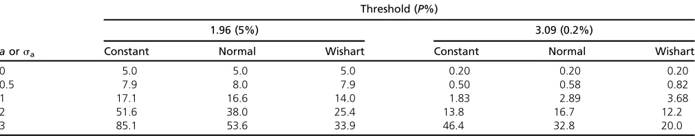
The mean numbers detected of 100 traits analyzed when both the gene effects and the error effects are uncorrelated are shown in Table 1 for three models of trait effect, namely constant (sa= 0;i.e.,ai= a, alli, included for reference),

normally distributed, and reﬂected Wishart-distributed gene effects. There is a high probability that real effects are missed even ifaiorsa= 2,i.e., 2 SD(ei). With a leptokurtic

distribution of effects, relatively more are missed than for the normal, particularly if the variance of effects is large and the threshold is low because many more genes have small effect. Absence of pleiotropy cannot be simply inferred solely from the results of tests of signiﬁcance.

If genes have correlated trait effects, whether overall or within modules, the probability an individual trait is detected and the mean number of traits detected is un-changed. The distribution of the numbers detected depends on the correlations, however (Figure 1). As the overall cor-relation, ra, of effects increases, so the distribution of

num-bers detected widens, as it becomes increasingly likely that very few or very many are detected. A correlation within modules, rma, has a qualitatively similar but quantitatively

Table 1 Expected numbers of traits testing signiﬁcant assuming 100 traits having constant effects (a) or uncorrelated normal or Wishart distributed random effects with SD =sa(by simulation)

Threshold (P%)

1.96 (5%) 3.09 (0.2%)

aorsa Constant Normal Wishart Constant Normal Wishart

0 5.0 5.0 5.0 0.20 0.20 0.20

0.5 7.9 8.0 7.9 0.50 0.58 0.82

1 17.1 16.6 14.0 1.83 2.89 3.68

2 51.6 38.0 25.4 13.8 16.7 12.2

3 85.1 53.6 33.9 46.4 32.8 20.0

(4)

much smaller inﬂuence. Correlations among the errors have less inﬂuence than among gene effects in these examples becausesa.1.

The shape of the distribution and consequently its mode are most affected when there is an overall correlation of gene effects (Figure 1). With a modular structure, the de-gree of skew of the distribution lessens as the number of modules increases (Table A1). Skew as illustrated by the mode becomes most extreme at high thresholds and with the leptokurtic distribution.

Pleiotropic effects of detected loci

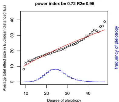
Wanget al.(2010) and Wagner and Zhang (2011) note that the Euclidean distance,TEz=O(Si=1,mzi

2_),_i.e._{, the root sum}

of squares of themdetected (i.e., signiﬁcant) effects, would be expected to be proportional toOmif there is no relation between the magnitude of detected effects and the degree of pleiotropy (i.e., the average effect of a locus on each trait is constant). Under this assumption the coefﬁcient ofmin the power curveTEz=cm

b_{would then be}_b_{= 0.5.}

This curve was ﬁtted to our simulated data, using both untransformed data and a weighted linear regression of log

TEz onm. Both yielded very goodﬁts as measured by R2,

typically.0.95, but the actual curve can depart consistently from the simple power curve (Figure 2). At high numbers detected, the best-ﬁtting power curve underpredicts, but these infrequent points get little weight. Similar departures are seen in some analyses of the real data (Wanget al.2010, Figure 3; and Wagner and Zhang 2011, Box 4).

The simulation results (Table 2) show that an exponent (b) ofTEzin excess of 0.5 can be obtained if there is a

cor-relation of effects or of the error, whether they are overall or within modules. Indeed, this statistic shows only that

pleiotropy is present but tells little about its structure be-cause it is insensitive to the correlations unless they are very small.

Pleiotropic effects of detected loci at the genotypic level:

Effects are detected when the phenotype (z) exceeds the threshold, but the genotypic effect (a) for a signiﬁcant trait is expected to be lower than z because the expected envi-ronmental deviation of those above the threshold is also positive (equivalently, the regression baz ,1). The

Euclid-ean distanceTEafor the genotypic effects for each correlated

trait declared signiﬁcant was also computed. The regression ofTEaonmrises more rapidly than doesTEzand can exceed

1.0, whether the correlations are across or within modules (data not shown), because the regression ofaonzincreases assa2increases.

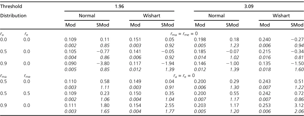
Modularity

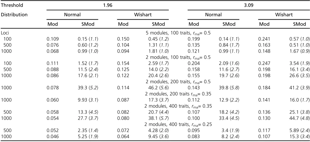
For the model used previously with 100 traits and 100 loci in five modules of equal size, estimates of modularity and scaled modularity are given in Table 3. These show that correlations among all traits do not generate much larity; indeed, higher correlations can lead to lower modu-larity. If correlations within modules are sufficiently high, in these examples.0.5, substantial scaled modularity can be generated. The modularity increases with the threshold and kurtosis of distribution of gene effects. Both the modularity and scaled modularity decrease as the correlation across modules becomes higher, but scaled modularity increases while modularity remains roughly unchanged if the correla-tion is within modules. As the number of traits or the num-ber of loci is increased (Table 4), modularity falls and scaled modularity increases, with the latter reaching high values. Figure 1 Distribution of numbers of traits declared to have a significant

effect. Model: 100 traits inﬁve modules with 5000 replicates (loci). Gene effects on traits follow a normal distribution with the threshold set at 3.09 (P= 0.2%). SD(ai)/SD(ei) =sa= 2. Correlations are ordered (ra,re,rma, rme). The mean number of traits declared signiﬁcant is 17 for all the

correlations displayed. The modes are 6 and 8 for (ra, re, rma, rme) =

(0.5 0.5 0 0) and (0.5 0 0 0), respectively, but are16 for the other examples.

(5)

Discussion

We are not arguing here that there may not be restricted pleiotropy or modularity of gene action, but that the sta-tistical evidence has to be considered critically. In particular we point out that a simple appearance of restricted numbers of traits shown to be signiﬁcant can simply be a consequence of sampling error and high threshold on variable effects among traits, and the thresholdP-values used here are much lower than if corrections were made for multiple testing. Thus Wagner and Zhang (2011) give a theoretical example for a study with 30 traits examined with a power of 80%. If signiﬁcant effects were found for 3 of them, the probability that 27 effects of the same or larger size are missed is,(12 0.8)27₁₀219_{. So they conclude that, if the power is 80%}

and few effects are detected, it is unlikely the true number is much higher;i.e., the detection bias is likely to be small in well-designed studies. We think this conclusion is overstated and the potential bias is severe. In their example, if the effects for all traits are actually the same and those missed

are due only to sampling error, the probability that no others are missed is 0.827_{0.0024, and the expected number of}

traits missed is 27 · 0.2 5,i.e., more than the number detected.

Hence the magnitude of actual pleiotropy is inevitably underestimated unless some alternative steps are taken. The use of basic trait data would considerably improve any analysis and we recommend this be done rather than merely judging signiﬁcance, especially when thresholds are high so the binary information is a small fraction of that in the actual records. Information on sign can also be lost. We consider it would be better to assume a joint distribution of effects of loci on the traits and attempt to estimate parameters of it. This would not be easy, but there is opportunity to set prior distributions and testﬁt in some kind of iterative structure. Any further analysis is well beyond the scope of this article, however.

We also consider the evidence that the power curve of effects as measured by Euclidean distance that shows the Table 2 Mean Euclidean distanceTEzfor total detected phenotypic effects for each mutant expressed in terms of number of signiﬁcant traits (m) for speciﬁed threshold levels

Threshold 1.96 3.09 1.96 3.09

Distribution N W N W N W N W

Correlations rma=rme= 0 ra=re= 0

ra re b rma rme b

0.0 0.0 0.50 0.50 0.50 0.51

0.0 0.5 0.61 0.43 0.54 0.50 0.0 0.5 0.54 0.47 0.52 0.50

0.5 0.0 0.74 0.81 0.57 0.61 0.5 0.0 0.73 0.85 0.58 0.65

0.5 0.5 0.73 0.71 0.56 0.59 0.5 0.5 0.74 0.77 0.58 0.63

0.75 0.0 0.71 0.74 0.56 0.60 0.75 0.0 0.75 0.87 0.59 0.65

0.9 0.0 0.67 0.69 0.55 0.59 0.9 0.0 0.74 0.85 0.58 0.65

There are 100 loci inﬁve modules withsa= 2 for normal (N) and for Wishart (W) distributed effects. Correlations of effects of gene and error effects are, respectively,raandre over all andrmaandrmewithin modules. Results are expressed in terms of the parameterbof the bestﬁt [estimated by weighted regression of logTEz= logc+blogm(R

2_. 0.97)] ofTEz=cmbto the simulated data. Means of 10,000 replicates are shown.

Table 3 Inﬂuence on modularity (Mod) and scaled modularity (SMod) of distribution and correlations of effects for a model of 100 traits and 100 loci inﬁve modules, each of 20 traits

Threshold 1.96 3.09

Distribution Normal Wishart Normal Wishart

Mod SMod Mod SMod Mod SMod Mod SMod

ra re rma=rme= 0

0.0 0.0 0.109 0.11 0.151 0.05 0.198 0.18 0.240 20.27

0.002 0.85 0.003 0.92 0.005 1.23 0.006 0.94

0.5 0.0 0.105 20.77 0.141 20.05 0.185 20.07 0.215 20.34

0.004 0.86 0.006 0.92 0.014 1.02 0.016 0.81

0.9 0.0 0.090 23.80 0.117 21.94 0.146 21.00 0.135 21.50

0.005 0.85 0.012 1.39 0.012 1.39 0.018 1.60

rma rme ra=re= 0

0.5 0.0 0.110 0.58 0.149 0.04 0.200 0.29 0.243 0.51

0.003 1.11 0.003 0.91 0.006 1.30 0.007 1.22

0.5 0.5 0.109 0.23 0.150 0.35 0.200 0.55 0.242 0.72

0.002 1.06 0.004 1.04 0.007 1.17 0.007 0.86

0.9 0.0 0.111 1.80 0.154 2.55 0.203 1.17 0.253 3.12

(6)

magnitude of effects increases with the degree of pleiotropy is not well founded. A gene that has a large effect correlated across traits is likely to be detected for more traits, so there is a nonrandom association between rate of detection and mean effect. It doesnotimply that ones of larger effect show more real pleiotropy as the degree of pleiotropy is the same for all pairs of loci in the model used here. The relationship between mean and mode of numbers detected is indicative of widespread pleiotropy if the mode is much smaller than the mean. This relationship is more extreme in theabsenceof modularity. Thus the more extreme distributions noted by Wagner and Zhang (2011) (e.g., their Figure 3B) are indic-ative more of correlations of gene effects across all traits than of correlations within modules.

The strongest evidence for modularity of gene action is undoubtedly provided by the speciﬁc analysis of networks. Correlation of effects as in a modular structure does indeed generate such evidence, albeit simulated assuming a model of universal pleiotropy with variable correlated effects. We do not doubt that the results cited by Wagner and Zhang (2011) show modularity of gene action, but we can simulate such results merely by assuming there is a moderate corre-lation of effects among loci, even though there is universal pleiotropy. To assess the sampling properties of the modu-larity and scaled modumodu-larity, sets of data were sampled using the same parameter values (number of genes, traits, and correlations). The results showed that the variation in the modularity is rather low relative to its mean, whereas that in the scaled modularity is relatively much larger. This indi-cates that, though scaled modularity has high sampling error when the system is small, the modularity is more robust.

Therefore our results indicate that large values of scaled modularity (e.g.,.10) as obtained by Wanget al.can arise with large data sets with a fully pleiotropic model, even if the correlation within modules is #0.5. The simulations show that the high values of modularity they obtained (.0.2 say) are more likely in our model if there are large correlations within modules, high threshold values, high kurtosis of dis-tribution of gene effects, and low variance of gene effects (i.e., lowsa).

Taken together with the lack of evidence for a relation-ship between the degree of pleiotropy and signiﬁcance of effects, it implies that we have to be wary of drawing con-clusions about lack of evolutionary constraints. A deeper analysis is required.

Literature Cited

Barber, M. J., 2007 Modularity and community detection in bi-partite networks. Phys. Rev. E Stat. Nonlin. Soft Matter Phys. 76: 066102.

Fisher, R. A., 1930 The Genetical Theory of Natural Selection, Ox-ford University Press, OxOx-ford.

Keightley, P. D., and D. L. Halligan, 2009 Analysis and implica-tions of mutational variation. Genetica 136: 359–369.

Mackay, T. F. C., 2010 Mutations and quantitative genetic varia-tion: lessons from Drosophila. Philos. Trans. R. Soc. B 365: 1229–1239.

Maslov, S., and K. Sneppen, 2002 Speciﬁcity and stability in to-pology of protein networks. Science 296: 910–913.

Orr, H. A., 2000 Adaptation and the cost of complexity. Evolution 54: 13_–20.

Stearns, F. W., 2010 One hundred years of pleiotropy: a retrospec-tive. Genetics 186: 767_–773.

Table 4 Inﬂuence on mean modularity (Mod) and scaled modularity (SMod) of changing the number of loci (equivalent to replicates), number of traits, module size, andrma

Threshold 1.96 3.09

Distribution Normal Wishart Normal Wishart

Mod SMod Mod SMod Mod SMod Mod SMod

Loci 5 modules, 100 traits,rma= 0.5

100 0.109 0.15 (1.1) 0.150 0.45 (1.2) 0.199 0.14 (1.1) 0.241 0.57 (1.0)

500 0.076 0.60 (1.2) 0.104 1.31 (1.1) 0.135 0.84 (1.7) 0.163 0.51 (1.0)

1000 0.068 0.99 (1.0) 0.094 1.81 (1.0) 0.121 0.99 (1.1) 0.148 1.67 (0.9)

2 modules, 100 traits,rma= 0.5

100 0.111 1.52 (1.7) 0.154 2.59 (1.7) 0.204 2.09 (1.6) 0.247 3.54 (1.9)

500 0.088 11.5 (2.4) 0.125 14.0 (2.2) 0.158 11.6 (2.7) 0.198 16.1 (3.4)

1000 0.086 17.6 (2.1) 0.122 20.4 (2.6) 0.155 19.7 (2.6) 0.198 26.6 (3.5)

1000 0.078 39.3 (5.2) 0.114 46.2 (5.6) 0.143 39.8 (5.8) 0.184 41.2 (3.9)

2 modules, 200 traits rma= 0.35

1000 0.060 9.93 (3.1) 0.087 17.3 (3.7) 0.112 12.9 (2.2) 0.141 16.0 (1.7)

500 0.058 13.3 (4.5) 0.082 20.7 (4.4) 0.107 18.2 (4.2) 0.136 25.1 (3.8)

1000 0.054 27.7 (3.7) 0.080 38.1 (5.7) 0.100 33.4 (4.5) 0.130 44.7 (4.8)

500 0.052 2.35 (1.4) 0.072 4.28 (2.0) 0.095 3.4 (1.9) 0.117 5.89 (2.4)

1000 0.046 5.25 (1.9) 0.064 9.45 (3.6) 0.083 8.2 (2.4) 0.107 15.3 (3.4)

(7)

Wagner, G. P., and J. Zhang, 2011 The pleiotropic structure of the genotype-phenotype map: the evolvability of complex organ-isms. Nat. Rev. Genet. 12: 206–213.

Wagner, G. P., J. P. Kenney-Hunt, M. Pavlicev, J. R. Peck, D. Waxman

et al., 2008 Pleiotropic scaling of effects and the ‘cost of complexity’. Nature 452: 470–473.

Wang, Z., B. Liao, and J. Zhang, 2010 Genomic patterns of plei-otropy and the evolution of complexity. Proc. Natl. Acad. Sci. USA 107: 18034–18039.

Communicating editor: S. F. Chenoweth

Appendix

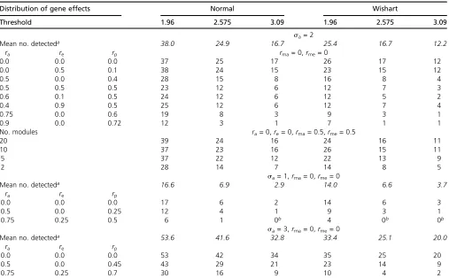
Table A1 Inﬂuence of correlations across and within modules on the mode of numbers detected

Distribution of gene effects Normal Wishart

Threshold 1.96 2.575 3.09 1.96 2.575 3.09

sa= 2

Mean no. detecteda _38.0 _24.9 _16.7 _25.4 _16.7 _12.2

ra re rp rma= 0,rme= 0

0.0 0.0 0.0 37 25 17 26 17 12

0.0 0.5 0.1 38 24 15 23 15 12

0.5 0.0 0.4 28 15 8 16 8 4

0.5 0.5 0.5 23 12 6 12 7 3

0.6 0.1 0.5 24 12 6 12 5 2

0.4 0.9 0.5 25 12 6 12 7 4

0.75 0.0 0.6 19 8 3 9 3 1

0.9 0.0 0.72 12 3 1 7 1 1

No. modules ra= 0,re= 0,rma= 0.5,rme= 0.5

20 39 24 16 24 16 11

10 37 23 16 26 15 11

5 37 22 12 22 13 9

2 28 14 7 14 8 5

sa= 1,rma= 0,rme= 0

ra re rp

0.0 0.0 0.0 17 6 2 14 6 3

0.5 0.0 0.25 12 4 1 9 3 1

0.75 0.25 0.5 6 1 0b ₄ ₀b ₀b

sa= 3,rma= 0,rme= 0

ra re rp

0.0 0.0 0.0 53 42 34 35 25 20

0.5 0.0 0.45 43 29 21 23 14 9

0.75 0.25 0.7 30 16 9 10 4 2

There are 100 traits.ra,re, andrp= (rasa2+re)/(sa2+ 1) are correlations across modules of gene, error, and“phenotypic”effects, and similarlyrma,rme, andrmpare correlations within modules.

a_{The mean number detected (numbers in italics) does not depend on the correlations. If, however, the correlations across module (}_r_a,_r_{e) are high, the probability that no}

traits are detected to be signiﬁcant rises, and the mean conditional on at least one trait detected may be much higher than shown.