University of Windsor University of Windsor
Scholarship at UWindsor
Scholarship at UWindsor
Electronic Theses and Dissertations Theses, Dissertations, and Major Papers
2008
Evaluation of machining systems from a complexity and cost
Evaluation of machining systems from a complexity and cost
perspectives
perspectives
Gabriel Gonzalez Gillis University of Windsor
Follow this and additional works at: https://scholar.uwindsor.ca/etd
Recommended Citation Recommended Citation
Gonzalez Gillis, Gabriel, "Evaluation of machining systems from a complexity and cost perspectives" (2008). Electronic Theses and Dissertations. 8091.
https://scholar.uwindsor.ca/etd/8091
EVALUATION OF MACHINING SYSTEMS FROM A COMPLEXITY AND
COST PERSPECTIVES
By
Gabriel Gonzalez Gillis
A Thesis
Submitted to the Faculty of Graduate Studies
through Industrial and Manufacturing Systems Engineering
in Partial Fulfillment of the Requirements for
the Degree of Master of Applies Science at the
University of Windsor
Windsor, Ontario, Canada
2008
1*1
Library and
Archives Canada
Published Heritage
Branch
395 Wellington Street Ottawa ON K1A0N4 Canada
Bibliotheque et
Archives Canada
Direction du
Patrimoine de I'edition
395, rue Wellington Ottawa ON K1A0N4 Canada
Your file Votre reference ISBN: 978-0-494-47048-0 Our file Notre reference ISBN: 978-0-494-47048-0
NOTICE:
The author has granted a
non-exclusive license allowing Library
and Archives Canada to reproduce,
publish, archive, preserve, conserve,
communicate to the public by
telecommunication or on the Internet,
loan, distribute and sell theses
worldwide, for commercial or
non-commercial purposes, in microform,
paper, electronic and/or any other
formats.
AVIS:
L'auteur a accorde une licence non exclusive
permettant a la Bibliotheque et Archives
Canada de reproduire, publier, archiver,
sauvegarder, conserver, transmettre au public
par telecommunication ou par Plntemet, prefer,
distribuer et vendre des theses partout dans
le monde, a des fins commerciales ou autres,
sur support microforme, papier, electronique
et/ou autres formats.
The author retains copyright
ownership and moral rights in
this thesis. Neither the thesis
nor substantial extracts from it
may be printed or otherwise
reproduced without the author's
permission.
L'auteur conserve la propriete du droit d'auteur
et des droits moraux qui protege cette these.
Ni la these ni des extraits substantiels de
celle-ci ne doivent etre imprimes ou autrement
reproduits sans son autorisation.
In compliance with the Canadian
Privacy Act some supporting
forms may have been removed
from this thesis.
Conformement a la loi canadienne
sur la protection de la vie privee,
quelques formulaires secondaires
ont ete enleves de cette these.
While these forms may be included
in the document page count,
their removal does not represent
any loss of content from the
thesis.
Canada
Bien que ces formulaires
AUTHOR'S DECLARATION OF ORIGINALITY
I hereby certify that I am the sole author of this thesis and that no part of this
thesis has been published or submitted for publication.
I certify that, to the best of my knowledge, my thesis does not infringe upon
anyone's copyright nor violate any proprietary rights and that any ideas, techniques,
quotations, or any other material from the work of other people included in my thesis,
published or otherwise, are fully acknowledged in accordance with the standard
referencing practices. Furthermore, to the extent that I have included copyrighted
material that surpasses the bounds of fair dealing within the meaning of the Canada
Copyright Act, I certify that I have obtained a written permission from the copyright
owner(s) to include such material(s) in my thesis and have included copies of such
copyright clearances to my appendix.
I declare that this is a true copy ozbzf my thesis, including any final revisions, as
approved by my thesis committee and the Graduate Studies office, and that this thesis has
ABSTRACT
Manufacturing systems, specifically machining, are typically designed as either
dedicated or flexible; representing two very different paradigms. Measures for
manufacturing flexibility have been proposed; generally, according to behaviour of
system or product mix. Attempts have also been made to relate flexibility to subsequent
costs.
In this thesis, System Design is presented as a property of inherent attributes determined
at the design stage. This provides the 'Flexibility Level' and its measurement is based on
physical-functional attributes. Hence, System Design is viewed as a continuous quality,
which describes both the level of flexibility and/or dedicated nature of a system.
This metric is related to cost in a model which describes system design in its entirety;
including manufacturing complexity in relation to cost as a tool to minimize
manufacturing costs. Consequently, system behaviour is investigated given alternate
manufacturing conditions such as varying product mix and production volume
DEDICATION
This thesis has been a major investment of time and effort but it is also a major
accomplishment. Support and encouragement has always been a critical driver necessary
especially through some difficult times.
I dedicated this work to two very important people in my life. First, my soon to
be wife, Kerri Charron, who has been patient to support all the time I have invested in
this effort. She has decided to stand by my side, provided strength and happiness; these
are the foundations for success.
I also dedicated this work to my mother, Deborah Gillis de Gonzalez. She has
always supported and pushed education upon her children. She has made it a priority for
us to strive to excel and I believe this work is culmination of her forming.
Lastly, some very important mentions of very important people that, even though
they are no longer with us, would have been extremely happy to share this moment and
the accomplishment. These are my aunt Lorie Cox, my grandmother Maria Luisa Roman
ACKNOWLEDGEMENTS
I will like to mention important individuals to whom I owe my most sincere
gratitude for their support and guidance through this work.
Dr. Hoda ElMaraghy and Dr. Waguih ElMaraghy have been significantly
important for the development of this thesis. First, their ready to lend a hand and
accommodating attitude has served as pillar where I have found the guidance needed to
develop this thesis. They believed an initial idea as presented and always held strong to
push to find and explore new avenues which complemented the effort. Their high
expectations were key for attained success.
Dr. Andrzej Sobiesiak was instrumental in given advice about starting this
program as well as for approaching potential program advisors. He has also provided
great advice as a member of my thesis committee. Dr. Baki has also been an active
participant in my committee meetings from where I have acquired great advice.
I will also like to express my appreciation to Aunt Ann for assisting in formatting
my work and Samin Shroki who has been a great friend and resource to discuss ideas and
TABLE OF CONTENTS
AUTHOR'S DECLARATION OF ORIGINALITY iii
ABSTRACT iv
DEDICATION v
ACKNOWLEDGEMENTS vi
LIST OF FIGURES ix
LIST OF TABLES xii
Chapter 1 Introduction 1
1.1 Flexible Manufacturing System Design Alternatives 3
1.2 Model for Manufacturing Flexibility Performance 5
Chapter 2 Literature Search 13
Chapter 3 Dimensions of Manufacturing Flexibility 21
3.1 Proposed Flexibility Scale Methodology 24
3.2 Example of Computation of Flexibility Scale 32
3.3 Next Dimension of Flexibility: Product Flexibility 34
Chapter 4 Complexity 41
4.1 Entropy approach or Shannon's Information 41
4.2 Effective Complexity 42
4.2.1 Computing Effective Complexity, KU(E), for Manufacturing Systems.... 44
4.2.2 Importance of Effective Complexity 48 4.2.3 Effective Complexity Application Example 51 4.3 Current Manufacturing Complexity Measures and Indices 57
4.3.1 Product Complexity 59 4.3.2 System Complexity 60 4.3.3 Process Complexity 70 4.3.4 Operational Complexity (Effort) 77
5.1 Implementation Effectiveness Strategy 88
5.2 Optimality Condition 90
Chapter 6 Cost function 92
6.1 FR1 = Target Jobs-Per-Hour (JPH; Production Rate) 94
6.2 FR2 = Capital Cost 95
6.3 FR3 = Operational Cost 96
6.4 FR4 = Changeover Cost & Agility 100
6.5 Cost Considerations vs. Product Variety (Mix) & Production Volume 102
6.6 Cost-Complexity Relation: After Runoff 108
Chapter 7 Application: Flexible-dedicated design 111
7.1 Grouping: Main approach for reduction of operation cost I l l
7.2 Product 115
7.3 Design Alternatives 115
Chapter 8 RESULTS & DISCUSSIONS 118
8.1 Future Research Opportunities 128
Chapter 9 CONCLUSIONS 129
9.1 Guidelines for Flexibility Implementation 130
REFERENCES 132
APPENDIX A: Proofs (Manufacturing Flexibility Model) 137
APPENDIX B: Proofs (Flexibility Scale) 138
APPENDIX C: Proofs (Product Flexibility) 140
APPENDIX D: Cost Function Discussions 141
APPENDIX E: Equipment Details 144
APPENDIX F: Cost Design Matrix Calculations 148
LIST OF FIGURES
FIGURE 1-1: EXAMPLES OF VINTAGE DEDICATED EQUIPMENT 4
FIGURE 1-2: EXAMPLES OF MOST ADVANCED FLEXIBLE TECHNOLOGY IN
USE TO DATE 4
FIGURE 1-3: COST VS. SYSTEM DESIGN 9
FIGURE 1-4: OBJECTIVE: COST VS. SYSTEMDESIGN APPLIED ON A
COMPLEXITY 9
FIGURE 2-1: STATION DESIGN - FLEXIBLE, DEDICATED (LICON MT L.P., 2006)
AND WEBZELL (APR 2005) 15
FIGURE 3-1: STRUCTURE OF FLEXIBILITY SCALE 24
FIGURE 4-1: CRANKSHAFT PIN-GRINDING MACHINING APPLICATION 53
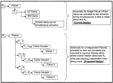
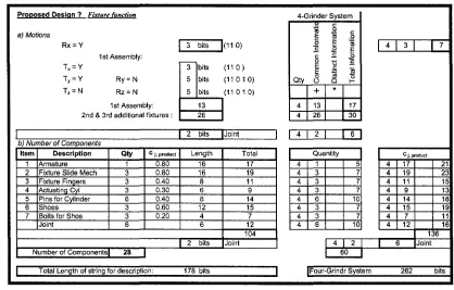
FIGURE 4-2: FIXTURE SYSTEM STRUCTURE 54
FIGURE 4-3: MANUFACTURING SYSTEMS CHARACTERISTICS AND
COMPONENTS (ELMARAGHY, H.A. 2006) 61
FIGURE 4-4: A COMPLETE MACHINE COMPLEXITY CODE (MCC) STRING FOR
AN EXAMPLE OF A MULTI-AXIS MULTI-SPINDLE MACHINE
(ELMARAGHY, H.A. 2006) 62
FIGURE 4-5: MANUFACTURING SYSTEMS EQUIPMENT COMPLEXITY CODE
(ECC) STRUCTURE (ELMARAGHY, H.A. 2006) 63
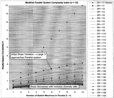
FIGURE 4-6: MODIFIED PARALLEL SYSTEM COMPLEXITY INDEX (EQUATION
9) — SMALL * X' 66
FIGURE 4-7: MODIFIED PARALLEL SYSTEM COMPLEXITY INDEX (EQUATION
9) — LARGE ' X' 67
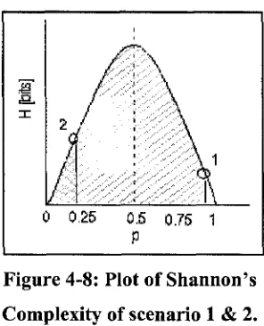
FIGURE 4-8: PLOT OF SHANNON'S COMPLEXITY OF SCENARIO 1 & 2 80
FIGURE 5-1: SYSTEM DESIGN MODEL 84
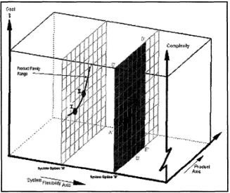
FIGURE 5-2: PRODUCT VS. COMPLEXITY PLANE: PRODUCT CATALOG &
SYSTEM RANGE 86
FIGURE 5-3: NOTE THAT (A) IS AN ASSUMED COST-DEMAND PLOT FOR
PRODUCT A; (B) IS THE PLOT FOR PRODUCT B WHICH HAS OPPOSITE
FIGURE 5-4: OVERALL APPLICATION PLAN 91
FIGURE 6-1: CUSTOMER NEEDS (CN) AND FUNCTIONAL REQUIRENMENTS
(FN) FOR SETUP OF COST MODEL 93
FIGURE 6-2: ZIG-ZAG AND DESIGN TABLE FOR FR1 = TARGET JPH 94
FIGURE 6-3: ZIG-ZAG FOR FR2 = CAPITAL COST 96
FIGURE 6-4: ZIG-ZAG FOR FR31 = OPERATIONAL COST: LABOUR COST 97
FIGURE 6-5: ZIG-ZAG FOR FR32 = OPERATIONAL COST: MAINTENANCE
MATERIALS 98
FIGURE 6-6: ZIG-ZAG FOR FR33 = UTILITIES 99
FIGURE 6-7: ZIG-ZAG FOR FR4 = CHANGEOVER COST AND AGILITY 100
FIGURE 6-8: SYSTEM DESIGN TABLE: IMPLEMENTATION & OPERATION
COST & AGILITY 101
FIGURE 6-9: COST REPORT CAD FOR DEDICATED SYSTEM 102
FIGURE 6-10: EFFECT OF PRODUCTION VOLUME ON COST PER SYSTEM
DESIGN (MEDIUM TO HIGH PRODUCTION) 105
FIGURE 6-11: EFFECT OF PRODUCTION VOLUME ON COST PER SYSTEM
DESIGN (LOW PRODUCTION) 106
FIGURE 6-12: COST VS. PRODUCTION VOLUME AND PRODUCT VARIETY.. 107
FIGURE 6-13: COST-COMPLEXITY BEHAVIOUR OVER TIME AFTER
EQUIPMENT RUNOFF 109
FIGURE 7-1: COMPOSITE PRODUCT MODEL - BLOCK "BOTTOM FACE" WORK
PLANE (M.B.C. AND OIL PAN BOLTS) 111
FIGURE 7-2: MOTION STACK-UP FOR AXES OF A SINGLE SPINDLE
MACHINING CENTER I l l
FIGURE 7-3: PRODUCT FAMILY SYMMETRY AND SPINDLE GROUPING 113
FIGURE 7-4: IMPROVED SPINDLE ADAPTER GROUPING 114
FIGURE 7-5: INDUSTRY AVAILABLE SPINDLE ADAPTERS (SHOU MING
INDUSTRIAL CO., 2007) 114
FIGURE 7-6: AUTOMOTIVE MACHINING PRODUCT CATEGORIES 116
FIGURE 7-7: MOTION AND CUTTING APPLICATIONS FOR GENERIC PRODUCT
FIGURE 7-8: ALTERNATIVE MACHINE ARRANGEMENTS 117
FIGURE 8-1: SUMMARY OF COST VS. FLEXIBILITY LEVEL FOR DESIGN
OPTIONS A, B AND C 122
FIGURE 8-2: COST VS. PRODUCTION VOLUME (COMPETING SYSTEMS, NO
RECONFIGURATION) 123
FIGURE 8-3: COST VS. PRODUCTION VOLUME AND PRODUCT VARIETY.... 124
FIGURE 8-4: SUMMARY OF EFFECTIVE COMPLEXITY VS. SCC MEASURES
(INCREASED SENSITIVITY) 126
FIGURE 8-5: EFFECTIVE COMPLEXITY & SCC RESULT OF EQUIPMENT
COMPARISON 127
LIST OF TABLES
TABLE 3-1: DEFINITION AND HIERARCHY OF FLEXIBILITY (KOSTE, ETAL.,
1999) 21
TABLE 3-2: ELEMENTS OF FLEXIBILITY AND POTENTIAL INDICATORS
(KOSTE, ET AL., 1999) 23
TABLE 3-3: SCALE OF FLEXIBILITY 33
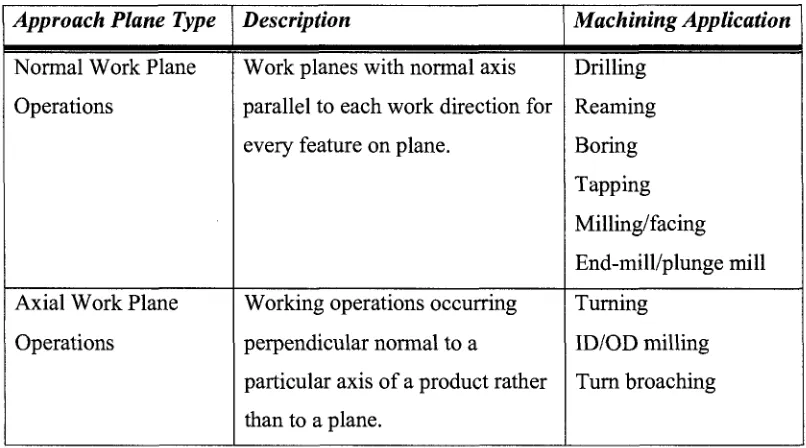
TABLE 3-4: PRODUCT GENERAL FLEXIBILITY WORK PLANES 38
TABLE 3-5: COMPOSITE PRODUCT MODEL - CYLINDER BLOCK 40
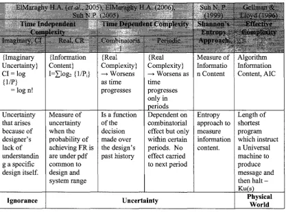
TABLE 4-1: SUMMARY OF COMPLEXITY 48
TABLE 4-2: EFFECTIVE COMPLEXITY OF PROPOSED NEW GRINDER DESIGN.
55
TABLE 4-3: DIMENSIONS OF MANUFACTURING COMPLEXITY 58
TABLE 4-4: MANUFACTURING SYSTEM EQUIPMENT CODES (ELMARAGHY,
H.A. 2006) 61
TABLE 4-5: SCC FOR ONE SINGLE-PIN VS. MODIFIED MULTI-PIN GRINDER. 68
TABLE 4-6: SCC FOR SYSTEM OF FOUR SINGLE-PINS VS. MODIFIED
MULTI-PIN GRINDERS 69
TABLE 4-7: SCC ANALYSIS OF DEDICATED DRILL-REAM-TAP OIL PAN &
M.B.C. BOLT HOLES 72
TABLE 4-8: EFFECTIVE COMPLEXITY RESULTS FOR DRILL + REAM + TAP
SYSTEM 72
TABLE 4-9: SCC ANALYSIS OF DEDICATED DRILL-TAP OIL PAN & M.B.C.
BOLT HOLES 73
TABLE 4-10: EFFECTIVE COMPLEXITY RESULTS FOR DRILL + TAP SYSTEM.
73
TABLE 4-11: SCC ANALYSIS OF FLEXIBLE DEDICATED DRILL-TAP OIL PAN &
M.B.C. BOLT HOLES 74
TABLE 4-12: EFFECTIVE COMPLEXITY ANALYSIS OF FLEXIBLE SYSTEM.... 74
TABLE 4-13: SCC ANALYSIS OF FLEXIBLE DRILL-THREAD MILL OIL PAN &
TABLE 4-14: EFFECTIVE COMPLEXITY ANALYSIS OF FLEXIBLE SYSTEM
WITH DRILL + THREAD MILL 76
TABLE 4-15: SCC ANALYSIS OF FLEXIBLE/DEDICATED DRILL-THREAD MILL.
77
TABLE 4-16: EFFECTIVE COMPLEXITY ANALYSIS OF FLEXIBLE-DEDICATED
SYSTEM WITH DRILL + THREAD MILL 77
TABLE 7-1: MOTIONS STACK-UP OF SINGLE SPINDLE C.N.C. MACHINING OF
COMPOSITE CYLINDER BLOCK - "BOTTOM FACE" 112
TABLE 7-2: REDUCED MOTIONS STACK-UP 113
TABLE 7-3: ASSUMED STRATEGIC PRODUCT OFFERINGS OF FIRM UNDER
ANALYSIS 115
TABLE 8-1: MANUFACTURING SYSTEM RESULTS - FLEXIBLE, DEDICATED
AND FLEX.-DEDICATED EXAMPLES 119
TABLE 8-2: COST REPORT CARD FOR DEDICATED SYSTEM 121
TABLE 8-3: COST REPORT CARD FOR FLEXIBLE SYSTEM (C.N.C. SINGLE
SPINDLE) 121
TABLE 8-4: COST REPORT CARD - FLEX.-DED. SYSTEM (C.N.C. W.
DEDICATED ADAPTER) 122
TABLE F-l: COST CALCULATION OF "DEDICATED SYSTEM" 148
TABLE F-2: COST CALCULATION OF "FLEXIBLE CNC - SINGLE SPINDLE". 151
TABLE F-3: COST CALCULATION OF "FLEXIBLE CNC -WITH DEDICATED
Chapter 1 Introduction
Manufacturing systems have been developed from their initial introduction in the
industrial revolution and through the mass production systems in the last century. The
development is characterized by the desire to push the limits of productivity and
manufacturing economy; this is still true to this day. The next challenge is presented by
ever increasing demanding customers and increase in market niches due to globalization.
Consumers have grown over past decades not only to expect affordable prices but also to
demand a level of quality and performance previously not achievable. In short, this
means that manufacturing systems now have three expectations: mass production prices,
competitive quality, and desirable and comprehensive product catalog. This is in contrast
to only cost being important to consumers as in the early 1900's.
Manufacturing technology has been developed from dedicated equipment to the flexible
C.N.C. (Computer Numerically Controlled) machining centers; both used today.
Nevertheless, either type of design presents its unique challenges for cost management of
high volume manufacturing. Transfer systems consist of highly non-responsive systems
composed of many dissimilar stations unique only to the individual process step.
Machining centers avoid this problem, hence making the system highly responsive to
changes. However, this type of system is usually expensive to operate and maintain.
The intention of this thesis is to address the comparison of both the dedicated and flexible machining systems. It is discussed that either of these systems are extreme cases of manufacturing system design. It is desired to understand which system is most economically beneficial for midrange to high volume manufacturing production. This is while establishing as the basis for analysis the attributes for individual station-system design.
It is presumed that manufacturing systems design can be compared by their level of
flexibility; this level is inherent to their initial design and is measured by a scale of
required. Each design alternative has a cost burden set by its designed flexibility and is
estimated with the manufacturing system's cost function. This establishes a relation
between flexibility and cost.
Furthermore, cost and manufacturing system complexity estimations are compared in a
proportionality relation. This is related by manufacturing system behaviour and
operational challenges, and it is useful as a tool for minimizing cost. All together, a
design model is assembled from these manufacturing system properties on a scale for
flexibility level. Assertions are made and a design strategy is developed for search of
economical designs.
The development of a unified model which describes a manufacturing system based on
total cost versus flexibility level is of extreme importance. It sets the stage for
minimization of cost for a varying level of flexibility. Thus, allowing trade-off of
flexible system designs and cost. It is believed that a refinement of the outlook of
manufacturing flexibility deployment, as proposed in this paper, will maximize its
observed benefits. It will drive economical design.
Therefore, objectives of this thesis are summarized as follows:
• Determine method to measure flexibility of a manufacturing system
• Develop unified system model to be used to described performance of
manufacturing systems in general and make assertions
• Use developed model to measure performance of sample manufacturing
systems with varying levels of flexibility design
• Incorporate Complexity Analysis into proposed design strategy
• Investigate behaviour of model after design and implementation
A fundamental development of the proposed design model is first introduced in
Section 1.2. All the definitions, relations, and rules required to build the model are
brought together. It is the foundation of the research. The design of a flexible
application but varying only in the level of flexibility implementation. That is,
application remains constant while the level of flexibility of the manufacturing system is
changed. Then, it is presumed that cost implication is a function related to the flexibility
of the system. The scale for measuring system flexibility is discussed in Chapter 3.
Chapter 4 discusses definitions of Complexity and its formulation to be used in
the design model. The design strategy is concluded in Chapter 5 with the introduction of
a 'product size' axis; furthermore, properties of system range, reconfigurability, and
design optimality are also discussed as applicable to the strategy.
Chapter 6 develops the manufacturing cost function. It is a practical description
of all the components of cost which are applicable from initial design, installation,
operation, possible reconfigurations and through final disposal of system. Thus, it infers
to total manufacturing costs. It is developed using Axiomatic Design. A cost report card
is developed and used for comparison of manufacturing system design alternatives.
Applications are given in Chapter 7, results and discussion in Chapter 8, and conclusions
in Chapter 9.
1.1 Flexible Manufacturing System Design Alternatives
Figure 1-1 and Figure 1-2 are examples of the extremes of dedicated and flexible
technology. Both system alternatives are used to process cylinder blocks but in two
completely different manners; each has its own advantages and disadvantages. Therefore,
developing a means of comparing and evaluating them is the intent. The discussion can
be enlightened by making the following questions. How would the cost distribution look
if the ninety six holes boring station of Figure 1-1 is replaced by a machining center as
the one in Figure 1-2? How would production schedules and required reconfigurations
Machining boring cases for automobile
engines at General Motors, 1937
Courtesy of Windsor Star, P8946 [10]http^/209.202.75.197/digi/sar/images/part 3/fordmarm facturing.jpg
3/25/2006
Manufacturing in Ford of Canada plant, 1915
Collection of Windsor's Community Museum, P8423
[l]tiltpy/209.202.75.197/digi/sar/images/part3/for d manu facturin s.jp g
Boring ninety-six holes simultaneously with a Foortburt boring machine, 1946
Courtesy of Windsor Star, P8945 {l]http://209.202.75.197/digj/sar/i mage s/part3/for
d manu factu ri ng.jp g
Figure 1-1: Examples of vintage dedicated equipment.
Stats from website: - "Completed in "one hit" the finished item took a little under 120 hours to machine using 58 tools & was our main demo on the MAM72-63V at EMO 2005.
- The MAM72-63V was developed with Motorsport & Automotive manufacturers & subcontractors firmly in mind, to give them a simultaneous 5_ axis machine that can work to impossibly tight tolerances on large & complex parts & components in one loading."
Typical HVL:
25 seconds/part; 144 part/hr; for effective ~650,000 parts/year
(17,280 parts per 120 hrs)
[2J V8 Cylinder Block - Machined From Solid, http-7/w" o.uk/news?action=view&newslD=41
1.2 Model for Manufacturing Flexibility Performance
Discussion in Chapter 3 will show how flexibility is not a single entity which
describes a quality of manufacturing system. Instead, it is understood as a property
applicable to many levels of manufacturing from the shop floor and up to the strategic
structure of a firm. Nevertheless, it is the combined effect of the application of flexible
policies at all levels which makes or breaks the advantage acquired by its application. For
example, consider two alternatives of poor application:
(1) Flexibility not used or when a system is well designed but by choice of
management only used for one product and marginal reconfiguration, and
(2) Flexibility limited by its design or when a system is only capable of operating
within a fraction of the total products in a family.
In contrast, a flexible system application can be of great benefit to the firm when a
successful flexible manufacturing system design is supported by a corresponding supply
chain capable of handling this flexibility. Furthermore, a product and release engineering
capable of following demands by marketing is essential.
This research is concentrated at the base level of a manufacturing firm: the shop floor.
This is not only where capital expenditure is most extensive but also where great effort
must be invested for changeover to new products. Here, a designer must work within
work-planes to design a manufacturing line. Individual stations are designed to produce
features in one work-plane. Further stations are added serially until all features within a
work-plane and all work-planes which make the product are covered.
The focus is to develop a method and/or guidelines for analysis at the station level. It is
to combine knowledge and experience with research to propose a structure for 'flexible
manufacturing' machining systems. In addition, this report will also propose guidelines
which must be met for good implementation. The reader should keep in mind that the
This section addresses the design model to serve as unifying-theory for all applicable
concepts. This is started by making reference to an important concept: productivity. The
following paragraph taken from the Accel-Team.com (2005) gives an enlightening
business perspective of this term.
"Essentially, productivity is the ratio to measure how well an organization (or individual, industry, country) converts input resources (labour, materials, machines, etc.) into goods and services.
This is usually expressed in ratios of inputs to outputs. That is (input) cost per (output) good/service. It is not on its own a measure of how efficient the conversion process is. "
Therefore, the following assembly 'A' is extracted from previous reference:
!A = Productivity
Al = applicable to an organization
A2 = Measure of performance
A3 = Ration of input (cost) per output (good/service)
A4 = Not measure of efficiency (of conversion process)
A similar statement should be inferred for manufacturing flexibility. Flexibility will
reach its full value when its effect can be related to a cost function. Thus, as productivity
relates to costs incurred by the production per unit produced, a scale of flexibility must
also relate cost to its extent of implementation. The future is the ability to distinguish
applications which are most cost effective and maximize strategic advantage. This is in
an attempt to avoid expensive practices. Therefore, from assembly ' B ' , Flexible
Manufacturing System (FMS) can be defined for intent of this thesis as follows:
1 For development of demonstrations I referenced first two chapters of "Theory of Sets" by (Bourbaki,
A Flexible Manufacturing System (FMS) is a quality, or alternative, of a
manufacturing system where it is designed to have some amount of flexibility (flexibility level); system has quality of being flexible. The system is then said it can react in case of changes whether predictable or unpredictable. Also, its application is done at many levels.
Definition extracted from following assembly ' B ' of definitions for Flexible
Manufacturing System (wikipedia.org, "flexible manufacturing system", 2007),
Flexible and Flexibility (Lexicon, 1988). See APPENDIX A(a) quoted statements.
B = Flexible Manufacturing System (FMS)
B1 = quality of a Manufacturing System
B2 = has some amount of flexibility (quality of being flexible)
B2, 1 = system can react in the case of changes
B2, 2 = predicted or unpredicted changes
B3 = has levels of application (i.e. machine, routing, etc.)
Cost of a Manufacturing System, from assembly 'C, is the aggregated costs
throughout the system's life cycle. Typical components of costs are installation or capital cost, operation (human, computing, etc), conversions or product upgrades, maintenance, and losses through inherent downtime.
C = Cost of manufacturing system
CI = aggregated cost
C2 = through system life cycle
C3 = of all components
C3, 1 = installation, capital cost
C3, 2 = operation (human)
C3, 3 = conversions, product upgrades
C3, 4 = maintenance
Also, it can be argued that, C depends on B, since manufacturing cost is dependent on the
design of the system. This is true in all manufacturing systems since incurred cost always
is greatly influenced by design options such as equipment type and numbers,
arrangements, distances, etc. This will also affect future operation burden. It said that,
C is a relation of B, C |B|,
Therefore,
Since it can be argued that when cost is considered for the entire life cycle of the system, it depends on the type of flexibility designed into the manufacturing system (flexibility level). Therefore,
Equation 1 Cost = /(Flexibility Level)
Chapter 3 will provide the required clarification on relating Manufacturing
System design and Flexibility Level. Briefly, Flexibility Level is proposed as a measure
of design of a manufacturing system based on its abilities. This distinguishes between
alternative levels of flexibility but does not make dedicated and flexible system
paradigms independent. It describes both; this gives any system the ability to be
dedicated or flexible as a continuous flow of design levels. Hence, design depends on
flexibility level. It is measured on a scale from ' 0 ' for dedicated equipment to ' 1 ' for
maximum flexibility ability.
Figure 1-3 illustrates the theoretical view of Equation 1. Here the system design
range is on the x-axis with dedicated to fully flexible systems at its extremes. Also
plotted in Figure 1-3 is a conceptual cost curve; it is an assumed approximation
applicable to high volume manufacturing. Arguably, cost maxima will occur at the
dedicated extreme since reconfiguration cost is high. Investment cost might also be high.
The low installation and reconfiguration cost in a flexible system is replaced by a high
L
t
Cost
\
\
t
0 Dedicated System
s
flexibility level —s>
/ /
/
1
1
t l Flexible System
Figure 1-3: Cost vs. System Design.
A complete model which describes total manufacturing cost is required. It is
desirable to find one that copes with alternate products (A, B, or C). Effectively, an
understanding of the behaviour of the cost optima according to flexibility level and
product changes is required. Furthermore, a manufacturing complexity variable is
introduced to illustrate the effects of increased complexity of both products and machines.
All this is illustrated in the updated model of Figure 1-4.
Complexity Whens,A«B<C
A
j * i
^ I I
i
l i
Design Flexibility Level ^
Figure 1-4: Objective: Cost vs. System Design applied on a complexity.
In context, Figure 1-4 implies that there exists proportionality between cost and
complexity of a system. This is illustrated in Assumption 1 which is the important tool
regarding manufacturing system behaviour are necessary to establish this relation.
Before, behaviour of a real manufacturing system is defined.
Manufacturing System Behaviour is the way in which a manufacturing system
behaves with respect to its original design intent and parameters. It is also the way it responds to its environmental influences: human operation, maintenance, tooling / materials, temperature-humidity, etc.
Ideal Manufacturing System Behaviour is deterministic. It refers to a system
which is predictable and controlled with certainty. It behaves according to its design and does not react to environmental influences.
Therefore, Manufacturing System Behaviour is an ensemble of elements or information; therefore, it depends on Physical Information, Effective Complexity, and Environmental Information, or Real or Imaginary Complexity. It directly affects performance.
In analogy to an ensemble, Manufacturing System Behaviour can be thought
of as an ensemble made up by random elements which contribute to the
overall performance. Consequently,
D2 = Manufacturing System Behaviour
Dl = Ensemble of elements (information)
D2 = Output is system performance
D3 = Elements (Information)
D3, 1 = Physical = Effective Complexity
D3, 2 = Environmental = Uncertainty and Ignorance
Behaviour is n. manners, deportment || moral conduct || the way in which a
machine, organ or organism works with respect to its efficiency || the way in
which something reacts to environment... (Lexicon, 1988).
Where,
E = Performance
El = property of something, system (applicable to task)
E2 = state of action; execution. Representation by action (completion)
E3 = what is accomplished, contrasted with capability (level of success)
E3, 1 = accomplish
= to bring to a successful conclusion, fulfill
Performance is a property of a system or task which is being executed. It is a
representation of the action and how well it is completed contrasted with capability. Thus, for a manufacturing system, the representation of how well the task of producing a product is measured by cost. Therefore, it is inferred that:
Y^Cost ~ Y£°
mpi
exity
Since Manufacturing System Behavior affects performance; complexity affects cost.
Assumption 1: Complexity-Cost Proportionality Relation
For any system of'/' sub-units made up by '_/' components, the sum of Cost and the sum
of Complexity components are proportional such that:
Equation 2 £ Cost ,y ~ ]T Complexity y
Furthermore, breaking into subcategories we obtain:
Equation 3
(Costij) i + (Costtj) 2 + ... = (ktj * Complexity ij) \ + (k,-y * Complexity u) 2+ —
Assumption 1: is important because it provides the means to bind Complexity theory to
Manufacturing Cost. Chapter 4 is a discussion of the knowledge necessary for
understanding of Complexity for practical purposes. It is a proficient tool for analysis
where other methods are limiting or might require great investment. Therefore,
Complexity can be used to increase understanding and control of systems. This is done
by means of managing information content of those variables which are unknown or not
Equation 2 may be modified by rearranging variables. Terms from either the cost
or complexity side are interchanged with their reciprocals. Thus, a complexity term can
replace a not well understood cost term. This will aid in the overall understanding and
manipulation of the final cost. The following assumption states this argument.
Assumption 2: Variable Interchange
Interchange reciprocal terms from cost or complexity sides of equation.
Equation 4:
(Cost ij) i + (k tj * Complexity ,7) 2 + ... = (k ,y * Complexity ij) \ + (Cost ,7) 2 + •••
Then, all that is left is the application of this tool. This is made clear with Assumption 3.
Assumption 3: Minimization of replaced variable
The effects of the replaced cost component are minimized by minimization of the
complexity term. Thus,
Equation 5: min {(Cost ij) 1} = min {(k i j * Complexity ij) 1}
In summary, the proposed approach is to use axiomatic design to generate a cost
function for all components of a flexible manufacturing system. Then, one can replace
Chapter 2 Literature Search
The task of establishing a relation between costs and manufacturing flexibility is
available in literature in varying degrees. Different aspects of flexible manufacturing are
approached; ranging from product mix, equipment layout, and product design among
others. Much evidence exists published in literature. Furthermore, several different
computation schemes for both cost and flexibility are available. However, a unification
model as one proposed in this thesis can serve to enhance research; great effort is spent in
this model to gather the necessary description to relate machining station design to
strategic plan of manufacturing firm. Some related articles are mentioned.
Complexity in General
Aldaihani {et al, 2005) provide an important example commonly present in
flexible systems in particular when common material handling systems is available
between stations. This is an example strongly related to scheduling complexity
discussion of Section 4.3.5. They present "a stochastic model to determine the
performance of a flexible manufacturing cell (FMC) under variable operational
conditions, including random machining times, random loading and unloading times, and
random pallet transfer times. The FMC under study consists of two machines, pallet
handling system, and a loading/unloading robot. After delivering the blanks by the pallet
to the cell, the robot loads the first machine followed by the second. Unloading of a part
starts with the machine that finishes its part first, followed by the next machine. When the
machining of all parts on the pallet is completed, the handling system moves the pallet
with finished parts out and brings in a new pallet with blanks."
Phukan {et al, 2005) propose complexity metrics for manufacturing control
architectures. "There is a need to develop metrics that quantify the complexity of a
stage. In this paper, we propose metrics used in software engineering to characterize the
complexity of manufacturing systems. These metrics have been applied for measuring the
Complexity of two software systems: material delivery system and distributed
scheduling." This is an interesting alternative to the discussions of Chapter 4.
An important concept which will be examined in later sections is the necessity
and importance of understanding product family and the effects this has on
manufacturing cost and flexibility agility. Suh E.S. (et al, 2007) expanded on this. "In
this paper, a multidisciplinary process for designing flexible product platform
components is introduced, assuming the platform component is decided a priori. The
design process starts with identification of uncertainties and generation of multiple design
alternatives for embedding flexibility into the component. Design alternatives are then
optimized for minimum cost, while satisfying the component performance requirements.
The flexible designs are then evaluated for economic profitability under identified
uncertainty."
Measure of Flexibility
Groote (1994) sets on finding a general framework for the modeling an analysis of
flexibility. It is based on the identification of three elements: the set of technologies
whose flexibility is to be compared, the sets of environments in which those technologies
might operate, and the performance criterion for the evaluation of the technologies. For
purpose of the discussion, Groote (1994) defines flexibility as:
"DEFINITION (flexibility as a complement to diversity). Technology *i e 7 is said
to be more flexible than technology ** 6 T(*s MJ> if for any pair of environments «u^<=B
such that ** «** *t> the following inequality holds:
wtft. «i> - *(*t# «») * * ( I J / *i) ~ *ih, «*)•»
This definition relates flexibility with an environmental response. Effectiveness is
Aksin (et ah, 2007) review the flexibility question. "The objective is to identify
preferred flexibility structures in service or manufacturing systems, when demand is
random and capacity is finite. Considering a network flow type model as the basis of the
analysis, general structural properties of flexibility design pertaining to the marginal
values of flexibility and capacity are identified."
Equipment Design (flexibility) and Cost
Figure 2-1: Station Design - Flexible, Dedicated (LiCON MT L.P., 2006) and Webzell (Apr 2005).
Akturk (et ah, 2006) propose a cellular manufacturing system design model to
manage product variety by integrating with the technology selection decision. The
proposed model determines the product families and machine groups while deciding the
technology of each cell individually. In order to integrate the market characteristics in
their model, they proposed a new cost function. The design process introduced is based
on two matrices one to describe 'machine capability, MCM', and a second to describe
'part requirements, PRM' for processing. Both are identity matrices composed of 0's and
The effort then consists of comparing between predetermine flexible and dedicated
operations to find best selection and arrangement. Flexibility of an entire cell is varied by
selecting between either alternative for each step. Selection of most economical cell is
made by ranking the totals for all pre-calculated cost indices. Ability to handle all
available products is also considered. Both, Akturk {et al, 2006) and this thesis are
inline for identifying a relationship between flexibility vs. cost. However, Akturk {et al,
2006) is focused on a higher level, cell design, than this report is, station design.
Freiheit {et al, 2007) investigate the investment and operational cost differences
between high volume serial and parallel C.N.C.-based machining lines. This study
provides insight into the cost-benefit tradeoff of implementing parallelism; that is, effects
of production line layout of flexible systems on machine reliability, line balance,
configuration throughput, and cost yields.
Kurtoglu (2004) explores a method for modeling and comparing between
alternatives of flexible assembly stations. A 'Total Cost, T C function is the basis of
comparison. It depends on matrices describing Flexibility of Workstation, F W (one for
setup cost and a second for resetting costs), Productivity, Operation Needs, Setup (current
state), etc. The values in these matrices are pre-calculated and either denotes time or cost
considerations.
Comparison is possible once the Total Cost function is determined for each system
variant. Production rate vs. cost plots from TC are then used to find optimum production
rate and costs for each system variant. This reference does not consider the detailed
behaviour of a station. The method for distinguishing flexibility is limited.
"It is important to determine an appropriate level of flexibility in the
reconfiguration of production systems while considering the tradeoffs between its costs
and benefits. This paper develops a real-option theoretical model that provides insights
method is presented to assist the justification of an RMS in deciding how to influence its
operating environment and choose right reconfiguration technologies in order to
maximize the performance measure of profitability." (Du, et al, 2006)
The analysis in Du {et al, 2006) is based on the following. "According to de Groote
(1994) general framework, in planning flexibility strategy with an RMS involves two
types of decisions:
1. Let G = {e|e = 1, . . . , E} be the set of all environmental factors upon which the
RMS is operated and which in turn influence the RMS.
2. Let F = { f | f = l , . . . , F } b e the set of all possible reconfiguration technologies
from which an RMS can be implemented.
The implementation of an RMS involves both a production environment and
reconfiguration technologies. Let C(e) and C( f) represent the cost associated with
implementing an environment and a reconfiguration technology, respectively.
Further let p(e, f) be the performance criterion (called profit function), where p(e, f) can
be any real-valued function, i.e., p :G xF —>R. Therefore, the flexibility planning problem
can be stated as:
max p(e, f), G,F
Though the profit function, p(e, f), can in principle be empirically estimated, the
implications about the profit function are not as straightforward as suggested by the
properties of these functions (Jordan, et al., 1995). This paper proceeds with the
development of a real-option method to estimate the profit function for given
environment and reconfiguration technologies."
Evans {et al, 2004) proposed comparison of competing flexible manufacturing
systems by the development of an Investment Analysis to review cost implications. This
is done for capital investment, variable cost structure and fixed costs on a net present
value over a five-year term and for each system option. The most profitable option is
Further development of investment analysis is proposed by Palmer (et ah, 2005). "The
proposed model better enables rational analysis of Flexible Computer-Integrated
Manufacturing (FCIM) system investment options, resulting in a more accurate
prediction of income and product line profitability attributable to FCIM system
investment."
Boyer (et ah, 1996) focuses on increased flexibility as a tool to address the
challenges posed by variable demand. This is done by examining two types of flexibility:
process and machine flexibility. The first is defined as the ability of a single
manufacturing plant to make more than a single type of product. Machine flexibility is
defined in terms of changeover cost (capacity or production loss). Further development
consists of relating product mix, plants, capacity at plants, and average demands.
Example: Table 3 from Boyer (et ah, 1996). This research does not sufficiently detail
individual station parameters.
Turkcan (et ah, 2007) review system design question with a dual objective:
minimization of cost and total weighted tardiness. "In this study, we consider flexible
manufacturing system loading, scheduling and tool management problems
simultaneously. Our aim is to determine relevant tool management decisions, which are
machining conditions selection and tool allocation and to load and schedule parts on
non-identical parallel C.N.C. machines."
Spicer (et ah, 2007) "Investigates how to determine the optimal configuration
path of a scalable-RMS that minimizes investment and reconfiguration costs over a finite
horizon with known demand.
- First, a practical cost model is presented to compute the reconfiguration cost
between two scalable-RMS configurations. This model comprehends labor costs,
lost capacity costs, and investment/salvage costs due to system reconfiguration
- Second, the paper presents an optimal solution model for the multi-period
scalable-RMS using dynamic programming (DP).
Third, a combined integer programming/dynamic programming (IP-DP) heuristic
is presented that allows the user to control the number of system configurations
considered by the DP in order to reduce the solution time while still providing a
reasonable solution."
Lau (et ah, 2004) propose a framework to be used for manufacturing system design.
"This framework aims at providing a unified platform for complex manufacturing
systems with enhanced formality. Features include procedures for requirement analysis,
simulation of system behaviour, and formal verification of abstract implementation. The
proposed framework helps to shorten lifecycle for system design and helps engineers to
produce manufacturing systems that conform better to original specifications to better
quality".
Furthermore, Boyle (2004) suggests a management strategy for implementation of
flexible manufacturing. "The purpose of this research is to develop a framework and an
initial list of best management practices for implementing manufacturing flexibility. To
identify these practices, recent frameworks (i.e. 1988 and onward) for implementing
manufacturing flexibility in organizations are reviewed. Based on this review, the major
management practices for implementing flexibility are identified and synthesized into a
new framework.
This framework suggests that manufacturing flexibility should be implemented using a
three-stage approach, labeled: identifying required flexibility (i.e. identifying and
justifying the flexibility types, measurements and tools needed to achieve the required
manufacturing flexibility), achieving required flexibility (i.e. acquiring and implementing
the organizational and technological tools needed to achieve the required manufacturing
flexibility) and managing required flexibility (i.e. monitoring and changing the required
flexibility types and levels, in light of changing uncertainty and competitive,
best management practices are identified." This paper is of interest since it mirrors the
efforts proposed in this thesis but from a management perspective rather than system
design.
Van Biesebroeck (2007) presents an overview of cost of flexibility. It "provides
evidence that while flexibility has an advantage to cope with increasing variety, there are
non-negligible costs as well".
Flexible-dedicated equipment design
Examples of creative equipment design and which are also directionally related to ideas
proposed in this thesis are found in literature. That is, the use of flexible-dedicated design
as an alternative to pure flexible or dedicated systems. Some examples are Lorincz
(2006), LiCON MT L.P. (2006) and Webzell (Apr 2005). The last two are reviewed
earlier in this section. Furthermore, the review by Webzell (Feb 2005) also provides
flexible cell designs which have flexible-dedicated attributes. Thus, providing further
prove that the technology described in this thesis is already under development. This
makes an excellent case for the necessity of model presented. That is, to provide a
roadmap for future implementation and research that speeds development and minimizes
risk of failure. The last example of equipment design to be mentioned is presented by
Chapter 3 Dimensions of Manufacturing Flexibility
A method for distinguishing between flexible manufacturing system designs must be
establish first before attempting to compare among alternatives. This must consist of a
qualitative metric, which describes system design from flexible to dedicated
arrangements. Thus, discussion in this Chapter begins with a summary of researched
material into the meaning of flexibility in manufacturing.
Manufacturing flexibility implementation varies at different levels of the firm but
each is important. For example, plant level design is a characteristic which contributes to
flexibility. In turn, it is independent of logistics planning but both are critical and must
be designed together. Both must meet the high level strategic plan of the firm.
Therefore, a firm's Flexible Manufacturing System (FMS) strategic implementation plan
must consider the 'top-to-bottom' structure of the organization. In brief, we must
consider these characteristics as the 'dimensions of manufacturing flexibility' as discussed
by Koste and Malhorta (1999). In their discussion, an exhaustive research is conducted
among the available literature to distinguish what are considered as dimensions of
flexibility and the extent of research among each. Table 3-1 summarizes their findings.
Included are the tiers of a manufacturing firm at which each dimension is applicable.
Table 3-1: Definition and hierarchy of flexibility (Koste, etal, 1999).
Dimensions ! Description
1
2
Individual
Resource
[Tier 1]
Machine
Flexibility
Labour
Flexibility
The number and heterogeneity (variety) of operations a
machine can execute without high transition penalties or
large changes in performance outcomes.
The number and heterogeneity (variety) of
tasks/operations a worker can execute without incurring
high transition penalties or large changes in performance
3
4
5
6
7
8
9
10 Shop
Floor
[Tier 2]
Plant
[Tier 3]
Material
Handling
Flexibility
Routing
Flexibility
Operation
Flexibility
Expansion
Flexibility
Volume
Flexibility
Mix
Flexibility
New
Product
Flexibility
Modificati
on
Flexibility
The number of existing paths between processing centers
and the heterogeneity (variety) of material which can be
transported along those paths without incurring high
transition penalties or large changes in performance
outcomes.
The number of products which have alternate routes and
the extent of variation among the routes used without
incurring high transition penalties or large changes in
performance outcomes.
The number of products which have alternate sequencing
plans and the heterogeneity (variety) of the plans used
without incurring high transition penalties or large
changes in performance.
The number and heterogeneity (variety) of expansion
which can be accommodated without incurring high
transition penalties or large changes in performance
outcomes.
The extent of change and the degree of fluctuation in
aggregate output level which the system can accommodate
without incurring high transition penalties or large
changes in performance outcomes.
The number and variety (heterogeneity) of products which
can be produced without incurring high transition
penalties or large changes in performance outcomes.
The number and heterogeneity (variety) of new products
which are introduced into production without incurring
high transition penalties or large changes in performance
outcomes.
The number and heterogeneity (variety) of product
modification which are accomplished without incurring
Functional
[Tier 4]
Strategic
Business
Unit
[Tier 5]
outcomes.
R&D Flexibility
System Flexibility
Organizational Flexibility
Manufacturing Flexibility
Marketing Flexibility
Strategic Flexibility
It is still necessary to find a scale for each dimension to be used in future design of
industrial applications. Koste {et al., 1999) also set to find a framework for analyzing the
dimensions of manufacturing flexibility. They defined critical characteristics, or
elements, that must be applied to each dimension if one intends to completely describe
flexibility. Table 3-2 describes the four elements that comprise the domain of any
flexibility dimension. These elements are Range-Number N), Range-Homogeneity
(R-H), Mobility (M), and Uniformity (U).
Table 3-2: Elements of flexibility and potential indicators (Koste, et al., 1999). Elements ' Indicators
Range-number (R-N)
Range-heterogeneity
(R-H)
Mobility (M)
Uniformity (U)
Number of options (operations, tasks, products, etc.)
Heterogeneity of options (difference between operations,
tasks, products, etc.)
Transition penalties - time, cost, effort of transition
Similarity of performance outcomes - quality, costs, time, etc.
Koste {et al, 1999) discuss, 'Range' is described as the number of different
positions, or flexible options, that can be achieved for a given flexibility dimension. This
is designed as R-N (range-number). They also argued range may not be as objective as a
range and create a richer measurement of range (designate as R-H or
range-heterogeneity).
'Mobility' is the third element and it represents the ease with which the organization
moves from one state to another. It corresponds to the 'ease of movement' which uses
both time and cost to assess its impact (Koste, et al, 1999). (The term agility is
sometimes used instead of mobility.) The last element is 'Uniformity'. Given the
similarity of performance outcomes, the less flexible system will exhibit losses in
performance outcomes.
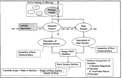
3.1 Proposed Flexibility Scale Methodology
Figure 3-1 describes the inner workings of the proposed Flexibility Scale. In
short, it is a bi-axis development that starts at the Firm's Catalog of Offerings where a
product family is extracted as a complete set. An idealized system which is capable of
handling all products within this family is built as the Industry Application.
Firm's Catalog of Offerings
Industry _ | Application
/ R e a l >v ~-V System
J-; Assembly of Root ! Characteristics
Flexibility Scale = Ratio of Abilities = Weight of Real System Weight of Ideal
Relative Comparison of Decision
1) Relative Magnitude of Decision
2) True/False Nature of Decision
A set of real system alternatives to be compared are also produced. A description for
both the Idealized and Real systems are developed using proposed methodology of Root
Characteristics. Finally, each real system alternative is ranked compared to the idealized
industry application. This is the Flexibility Level expressed as the Ratio of Abilities.
The methodology proposed as follows is applied at the lowest level (dimension) as
represented in Table 3-1; machine flexibility'. The first step for set-up of this analysis of
system flexibility is to make a determination on the 'product family' to be reviewed.
A = family
Al = group of elements
A2 = grouped by a common characteristic
B = Product
Bl = good which can be bought or sold (has value)
B2 = purchased as materials and sold as good (is produced)
Assembly C = Product Family, or Range Product Range
= given by assembly of characteristics A and B
= Characteristic of any one or group of object x
= AB(x)
Product Family, or Product Range, is a single or group of objects 'x'
characterized by a common characteristic, utility. Each having both commercial value or existing need, and is an item produced as result of a manufacturing activity .
D = Utility
Dl = State or act of using or being used (useful)
3 Method can be extended to provide scale for the remaining dimension of FMS.
4 Definitions utilized can be found in APPENDIX B(a)
D2 = function, the purpose for which is something is used (has function).
E = Property
El = is an attribute
E2 = common to elements of a group
E3 = cannot be used to distinguish between elements of a class
Therefore, from assembly of D and E; we consider utility as of set of objects x,
Utility of object, or group of objects x is first the state or act of having usefulness, which satisfies purpose and/or function. Secondly, group of products must be related by a common attribute(s) but which cannot be used for distinguishing between them.
This means, for example, that we might group elements of the family of cylinder blocks
having "counter-weighted cranks", "cylinder head(s)", and "piston-connecting rod" as
common characteristics. The distinguishing characteristics are size and arrangement (V
or I). These limitations are not applicable to Wankel rotary engines since crank is
replaced by a rotor, head by cover, and piston is non existent.
Note that a second terminology is used in this report as the 'catalog of offerings'; it is the
catalog which includes all product families offered by the firm (cranks, blocks, etc). Not
to be confused with product family.
The second step defines the guidelines for comparison. This is based on
comparing competing systems with respect to one another; relative comparison.
F6 = Decision
Fl = a definite selection
F2 = select one choice from set of alternatives
F3 = designated for an application (has related application)
G = Comparison
Gl = must have at least two elements or characteristics
G2 = must have expression of objects or characteristics (direct or
transformation) which allows determination of like/unlike
comparison (must be comparable)
H = Relative
HI = is object or characteristic of something (quantity, quality, truth, idea,
etc.)
H2 = is known only with respect to a second object or characteristic
H3 = is not absolute statement
Therefore, from assembly FGH and for this thesis,
Relative Comparison of Decision (or Relative Comparison) is a definite
statement or assertion which selects one alternative among many; these are related and satisfy a need.
These alternatives are expressions of objects or characteristics such as quantity, quality, truth, idea, etc., which assists in making determinations between them. However, no absolute statement exist and all is known is with respect to a second object or characteristic.
Two concepts of choice-decision are applicable:
1) Relative Magnitude of decision - This type of comparison is used to describe
features of flexibility having magnitudes of abilities. This is accomplished by using factors. These could be numbers such as 0, 1, 2, etc. Zero is for non-desirable and
higher numbers for increasingly advantageous systems.
J = Relative Magnitude Comparison
Jl = set of comparables
J l , 1 = is object or characteristic of something
J l , 2 = is a magnitude measurable
J l , 3 = there exists two or more objects
J2 = relation is non-absolute rather it is know with respect to a base of
comparison. (Use of factors)
2) True or False nature of decision - Objects or characteristic that are of
existence type. That is, they either exist or not; are available or not. The designation for this comparison is of binary type; values are (True = 1, False = 0). This addresses the general ability question: can the system cope with such: yes/no? Given by,
I = T / F Decision
11 = is a decision (as per previous discussion)
12 = is an existence characteristic
(It either exists or not; available or not)
The third step is to identify and list all available characteristics for a
system/industry application. The task is to achieve all root characteristics of a
manufacturing system. Care must be taken to avoid mixing similar options; thus,
achieving range-(number, heterogeneity) as per previous discussion
K7 = Root
Kl = is a statement of object or characteristic
K2 = is fundamental or essential
L = Characteristic
LI = quality of object
L2 = is distinguishable from other descriptions
M = Manufacturing System
Ml = Equipment
M l , 1 = Production Equipment
M l , 1, 1 = Operation Equipment
M l , 1, 1, 1 = Station equipment
M l , 1, 1, 1, 1 = Spindle
M l , 1, 1, 1, 1 = Slide(s) System
M l , 1, 1, 1, 1= Tooling
M l , 1,2 = Work Holding-Fixturing
M l , 2 = Material Handling Equipment
M l , 3 = Test Systems
M2 = Management Strategy (Flex., Quality System, etc)
M3 = Human Factors
Therefore, from assembly of KLM,
Root Characteristic of Manufacturing Systems is a statement of an object or characteristics which is an essential element of a description. It describes a quality which is unique and fundamental. It is the functional elements which make a manufacturing system. The alternatives in arrangements make the alternatives in manufacturing systems (flexible, dedicated).
For example, functional components of a machining application are: spindles, transfers,
slides, tools, etc. Once identification of all options is complete, it is time to set-up
evaluation. The basis for the proposed measure of manufacturing flexibility is given by
the measure of Total Abilities of an Industry Application. The description of an
industrial application is given by the assembly KLM applied to the manufacturing
equipment. That is, it is the set of 'root characteristics' which complete a description of a
system.
N = Industry Application
N2 = has intent of addressing a need
(Low/High Volume, Product Type, Size, etc)
N3 = inherent type (machining, assembly, stamping, etc)
An Industry Application is a set of manufacturing equipment of inherent type (machining, assembly, stamping, etc.) arranged to address a manufacturing need (Low/High Volume, Work Size, etc). A Description of Industry Application is the set of root characteristics without specifying arrangement.
Description of an industry application' is the assembly of KLM and N (KLMN(x));
where x is any equipment. Then, Total Abilities of an Industry Application are the sum
of the weights of all root characteristics identified in the description of industry
application. It is given by rankings I, J applied to assembly KLMN(x); it is assembly (IJ)
KLMN(x). That is,
0 = Weight of Root Characteristic
0 1 = Root Characteristic (1 through n); KLMN(x)
0 2 = Elements of Comparison
0 2 , 1 = Range-Homogeneity
0 2 , 2 = Range-Heterogeneity
0 2 , 3 = Uniformity
0 2 , 4 = Mobility
0 3 = Comparison Ranking; IJ
0 3 , 1 = T/F Comparison (Binary 0 or 1)
0 3 , 2 = Magnitude Comparison (Factors 0, 1, 2 ...)
0 4 = Max possible weight
Then, Total Abilities of an Industry Application is the weight taking the highest possible value for all ranks of all the root characteristics which make the entire description.
The fourth step is the final comparison of the system in question and the industry
application. Hereafter all is left is to unite all concepts introduced thus far and explain
how they form the scale for manufacturing flexibility. This is introduced as the Ratio of
Abilities; this is the scale.
Recalling the assembly KLMN(x) is a description of equipment x by assembly of all root
characteristics. Also, the rank is given by assembly (IJ) applied to KLMN(x) following
condition 0 2 . The weight is then the sum of all ranks for all characteristics.
Ratio of Abilities - Total Abilities is the weight calculated by summing all
maximum possible ranks; this can be considered as the number options available in an Industry Application. However, not all systems have the same abilities. They will have varying weights. Therefore, the actual weight of a system is defined as the 'Weight of a System'. Then, arguably, it is possible to deduce the comparison of a given system with the Industry Application as:
Flexibility Scale = Ratio of Abilities = Weight of a System
Total Abilities
Total Abilities is also understood as the weight of the system with maximum
possible options which describes a given product family. That is, the idealized
manufacturing system for a given product family, or Industry application, which