Gravitational waves from the dynamical bar instability in a rapidly rotating star - art. no. 084024.

Gravitational waves from the dynamical bar instability in a rapidly rotating star

J. David Brown

Department of Physics, North Carolina State University, Raleigh, North Carolina 27695-8202 共Received 31 March 2000; published 25 September 2000兲

A rapidly rotating, axisymmetric star can be dynamically unstable to an m⫽2 ‘‘bar’’ mode that transforms the star from a disk shape to an elongated bar. The fate of such a bar-shaped star is uncertain. Some previous numerical studies indicate that the bar is short lived, lasting for only a few bar-rotation periods, while other studies suggest that the bar is relatively long lived. This paper contains the results of a numerical simulation of a rapidly rotating␥⫽5/3 fluid star. The simulation shows that the bar shape is long lived: once the bar is established, the star retains this shape for more than 10-bar-rotation periods, through the end of the simulation. The results are consistent with the conjecture that a star will retain its bar shape indefinitely on a dynamical time scale, as long as its rotation rate exceeds the threshold for secular bar instability. The results are described in terms of a low-density neutron star, but can be scaled to represent, for example, a burned-out stellar core that is prevented from complete collapse by centrifugal forces. Estimates for the gravitational-wave signal indicate that a dynamically unstable neutron star in our galaxy can be detected easily by the first generation of ground based gravitational-wave detectors. The signal for an unstable neutron star in the Virgo cluster might be seen by the planned advanced detectors. The Newtonian-quadrupole approximation is used throughout this work.

PACS number共s兲: 04.30.Db, 04.40.Dg, 95.30.Lz, 97.10.Kc

I. INTRODUCTION

A self-gravitating, axisymmetric fluid body with a suffi-ciently high rotation rate can be dynamically unstable to non-axisymmetric perturbations. Typically, the fastest growing unstable mode is the m⫽2 ‘‘bar’’ mode which acts to trans-form the body from a disklike shape to an elongated bar that tumbles end over end. This instability has been described analytically for the case of uniform density bodies关1,2兴, and has been the subject of numerous numerical studies.1 The numerical results show that bar formation is accompanied by the ejection of mass and angular momentum, and that the ejected matter forms long spiral arms in the equatorial plane. The subsequent evolution is less certain. Some simulations indicate that the bar shape is short lived, with the star return-ing to a predominantly disklike shape after a few bar-rotation periods. Other simulations predict that the bar persists for many bar-rotation periods. In recent work, New, Centrella, and Tohline 关3兴 address this issue with a series of simula-tions using two different codes at various resolusimula-tions, and conclude that the bar shape is persistent. In their highest resolution run the bar decayed after roughly six or seven bar-rotation periods. This was believed to be caused by nu-merical errors that induced an unphysical center of mass mo-tion. In a lower resolution run a symmetry condition was imposed that prevented any center of mass motion. In that case the star maintained its bar shape throughout the simula-tion.

The purpose of the present work is to simulate the long-time evolution of a rapidly rotating, self-gravitating star us-ing Newtonian hydrodynamics and gravity. As discussed in Sec. III, the numerical code is substantially different from

the codes that have been used previously to address this problem. The initial data for this study consists of a␥⫽5/3 polytrope with stability parameter␤⫽0.30. The stability pa-rameter is defined by␤⫽T/兩W兩, where T is rotational kinetic energy and W is gravitational potential energy. The results here suggest that the bar shape is indeed long lived—the star displays a prominent bar shape at the end of the simulation, which includes more than ten bar-rotation periods.

Numerical studies of fluids with various equations of state and initial rotation profiles have shown that the dynamical bar instability appears when the stability parameter ␤ ex-ceeds a certain critical value, typically close to 0.27 关4,5兴. For the secular instability, which arises through dissipative mechanisms, the critical value of ␤ is near 0.14. A neutron star might reach the critical value of ␤ for dynamical or secular instability by accreting matter and angular momen-tum from a binary companion. A stellar core that has ex-hausted its nuclear fuel might reach a critical rotation rate as it collapses.

A star or stellar core that develops a rotating-bar-like con-figuration will generate large amounts of gravitational radia-tion. Depending on the distance of the source, this radiation might be strong enough to be detected by the worldwide network of gravitational-wave detectors currently under con-struction关6兴. Here, the question of the persistence of the bar shape becomes very important. The detectability of a source depends on its characteristic amplitude hc⬇h

冑

Should we expect the bar shape to persist or decay? One reason why the bar might decay is the loss of mass and angular momentum from the ends of the bar. The accompa-nying drop in rotational kinetic energy could reduce the sta-bility parameter and allow the star to return to axisymmetry.

1_{For a brief review, see Ref.关3兴.}

Loss of rotational kinetic energy through shock heating might also occur. For the simulation presented here,␤has an initial value of 0.30, large enough to dynamically trigger the growth of the bar mode. During the initial period of bar formation, mass and angular momentum are shed from the ends of the bar and long, spiral arms are formed. The stabil-ity parameter rapidly drops below 0.27 and eventually settles to a value of about 0.24. However, these losses of mass and angular momentum, with the accompanying drop in ␤, are insufficient to completely rob the star of its bar shape.

The results here are consistent with the conjecture that the star will retain its bar shape indefinitely on a dynamical time scale, as long as␤stays above the critical value for secular instability关8兴. If this is correct, the bar should still decay due to secular processes. Imamura, Durisen, and Pickett have ar-gued that the bar continues to shed small amounts of angular momentum to the spiral arms, and these losses cause the bar to decay 关8兴. Other secular mechanisms, such as energy and angular momentum loss through gravitational radiation, could play a role as well.

It is possible that, for the equation of state and angular velocity profile used here, the star is able to retain its bar shape simply because the critical value of ␤ for dynamical instability is 0.24 or less. This possibility was tested by con-ducting a second simulation using the same equation of state and scaling the angular velocity by a factor of 3/4. The re-sulting model has an initial value of␤equal to 0.25. The bar mode showed no signs of growth in this simulation. Thus, for the models tested here, the bar mode does not spontane-ously grow unless ␤ exceeds a critical value greater than 0.25. However, once the bar shape is established, it can per-sist for many bar-rotation periods with ␤ equal to 0.24 or less.

In the present numerical calculation there are two sources of error in angular momentum. First, some of the angular momentum that is lost off the edge of the computational grid might, ideally, fall back onto the star. Second, numerical errors at each time step introduce a purely artificial loss of angular momentum. Both of these errors act to decrease the angular momentum of the star. One expects such losses to cause the bar shape to deteriorate. What is seen, both in the gravitational wave analysis and in the Fourier analysis of the density, is a relatively persistent signal with a modest decline in amplitude over the duration of the simulation.

The physical model and initial data that form the basis of the simulation are described in Sec. II. Section III contains a discussion of the numerical code. The results of the simula-tion are described qualitatively and quantitatively in Sec. IV. Conclusions and results are summarized in Sec. V. Details of the initial data code are given in the Appendix.

II. PHYSICAL MODEL

The initial data for the simulation consist of a stationary, axisymmetric Newtonian fluid star with polytropic equation of state, P⫽K␳␥. The equation of state parameters are cho-sen to coincide roughly with those of a low-density neutron star with soft equation of state, ␥⫽5/3 and K⫽5.38 ⫻109cgs 关2兴. The bar instability in stellar cores with stiff

equations of state has been investigated by Houser and Cen-trella关9兴.

The equations of hydrostatic equilibrium are solved using an algorithm described in the Appendix, in which the freely specifiable data are the central density ␳_c and the angular velocity distribution ␻(r). Here r is the distance from the rotation axis. With the choices

␳c⫽2.00⫻10

14 _g/cm3_{, 共1a兲}

␻共r兲⫽共4000/s兲e⫺共r/4.80⫻106 cm兲2, 共1b兲

the equilibrium configuration has mass, equatorial radius, po-lar radius, angupo-lar momentum, and stability parameter given by

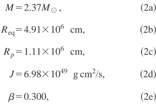
M⫽2.37M_䉺, 共2a兲

Req⫽4.91⫻106 cm, 共2b兲 Rp⫽1.11⫻106 cm, 共2c兲

J⫽6.98⫻1049 g cm2/s, 共2d兲

␤⫽0.300, 共2e兲

respectively. Equations 共1b兲 and共2b兲show that the angular velocity has values

␻共0兲⫽4000/s, ␻共Req兲⫽1400/s, 共3兲

on the rotation axis and at the equator. The azimuthal veloc-ity at the equator is 6.89⫻109cm/s, below the Kepler veloc-ity of 8.90⫻109cm/s. Note that the mass 共2a兲 is consider-ably larger than the masses of observed neutron stars, and exceeds the limit for nonrotating neutron stars for most equa-tions of state. However, as discussed by Baumgarte, Shapiro, and Shibata 关10兴, differentially rotating ‘‘hypermassive’’ neutron stars with M⬎2 M_䉺might appear as the immediate products of core-collapse supernovas or binary neutron star mergers.

The rotation law for a uniform density Maclaurin spheroid is

The dimensionful model described here can be rescaled by introducing parameters␭,␮, and␶that scale the lengths, masses, and times. To be precise, a quantity Q with dimen-sions关Q兴⫽LAMBTC, where L is length, M is mass, and T is time, is rescaled according to Qnew⫽Qold/(␭A␮B␶C). A physical, dimensionful model is retained if the parameters are dimensionless and Newton’s constant G is unchanged by the rescaling. This requires ␭,␮, and␶to satisfy␭3⫽␮␶2. Alternatively, the model can be converted to polytropic units

关12兴 in which G⫽K⫽M⫽1 by setting ␭⫽4.81⫻105cm, ␮⫽4.71⫻1033g, and␶⫽1.88⫻10⫺5s. This leads to

␳c⫽4.73⫻10⫺3, 共5a兲

Req⫽10.2, 共5b兲

␻共0兲⫽7.53⫻10⫺2_{, 共5c兲}

for the central density, equatorial radius, and central angular velocity.

For the model with the scaling displayed in Eqs.共1兲and

共2兲, the maximum flow velocity is 8.2⫻109_{cm/s. This} occurs at a distance of 3.4⫻106cm from the rotation axis. At this peak velocity, the special relativistic gamma factor (1⫺v2_/c2₎⫺1/2_{, where c is the speed of light, differs from} unity by about 4%. General relativistic effects should be greatest near the surface of the star at the poles, where the gravitational potential is approximately G M /R_p⫽2.8 ⫻1020cm2/s2. Comparing this result with c2, we find that general relativistic effects represent a correction of roughly 30% at the poles. Thus, with the scaling used in Eqs.共1兲and

共2兲, the errors that we introduce by ignoring special and gen-eral relativity are substantial.

The errors are reduced if the model is rescaled appropri-ately. For example, with␭⫽1/2,␮⫽2, and␶⫽1/4, the mass of the star is cut in half, its linear size is increased by a factor of 2, and its angular velocity is decreased by a factor of 4. In this case the model might represent a stellar core that has partially collapsed, but is prevented from contracting to

nuclear density by centrifugal forces. 共Note that with this scaling Newton’s constant is unchanged. Also note that the speed of light should not be scaled, since it does not appear in the Newtonian hydrodynamical equations or the Poisson equation.兲 The scaling reduces the maximum speed by a factor of 2 and reduces the gravitational potential by a factor of 4. For this model, special and general relativistic effects represent corrections of about 2% and 8%, respectively.

III. NUMERICAL CODE

The axisymmetric initial data were calculated on a grid in the r-z plane consisting of 512⫻511 zones. Details and tests of the initial data code are contained in the Appendix. In preparation for the evolution of this data, the grid was chosen to cover a physical domain of 1.77⫻107cm in radius and 2.50⫻107cm in the z direction. Thus the star was contained in a small region of the grid, roughly the inner 142⫻45 zones. The quality of the data can be checked with the diag-nostic expressionV⫽(2T⫹W⫹3兰P dV)/W, where T is ki-netic energy, W is gravitational potential energy, and 兰P dV is the volume integral of pressure. According to the virial equations, this quantity should vanish关1,13兴. For the numeri-cally generated model, this diagnostic has a value of V ⫽3.2⫻10⫺5.

At the beginning of the evolution, the density and velocity are interpolated onto a three-dimensional Cartesian grid. The grid contains 1283 zones and covers a cubic domain with sides of length 2.50⫻107cm. The equatorial radius of the star spans 25 zones, while the polar radius spans 6 zones. The density in each zone is modified with a random pertur-bation ranging from ⫺10% to ⫹10% of the unperturbed value. Initially, the specific internal energy e is obtained from the density by the relation e⫽K␳␥⫺1/(␥⫺1). There-after, the star is evolved with the equation of state

P⫽共␥⫺1兲␳e, 共6兲

with␥⫽5/3.

The evolution code includes the nonrelativistic hydrody-namics codeVH-1, written by Blondin, Hawley, Lindahl, and Lufkin. VH-1 is based on the piecewise-parabolic method

共PPM兲 as described by Colella and Woodward 关14兴. The PPM scheme is a higher-order extension of Godunov’s method 关15兴. It uses parabolas as interpolation functions within each zone and characteristics to determine the do-mains of dependence for zone interfaces. The average values of density, pressure, and velocity within these domains are used as inputs to the Riemann problem between adjacent zones. The solution of the Riemann problem determines time-averaged values of pressure and velocity, which in turn are used to compute hydrodynamical fluxes. In VH-1, each time step is reduced to three one-dimensional evolutionary ‘‘sweeps’’ via operator splitting. For each one-dimensional sweep, the fluid variables are evolved in Lagrangian coordi-nates and then remapped onto the original Eulerian grid. The order of the sweeps is cycled through all possible permutations.

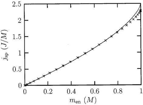
FIG. 1. The specific angular momentum jsp, in units of J/ M , versus the mass menenclosed in a cylindrical radius, in units of M. Both the numerical data共crosses⫻兲and the Maclaurin rotation law

For the simulation presented here, I used a ‘‘Courant number’’ of 0.3. That is, the time step was set to 0.3 times the maximum allowed by the Courent-Friedricks-Lewey

共CFL兲 condition. This is a relatively small time step for a PPM code. It was chosen to help minimize the artificial loss of angular momentum, discussed below.

The Poisson equation for the gravitational potential is solved using multigrid methods关16兴. The finest grid has size 1293, with grid points that lie at the corners of the 1283 hydrodynamical zones. The boundary conditions are com-puted from a multipole expansion of the potential that in-cludes monopole, dipole, quadrupole, and octupole terms.

The PPM method is designed to evolve the fluid mass density ␳, linear momentum density, and total energy den-sity, and in the process to conserve the mass, linear momen-tum, and total energy of the system. Unfortunately, for such a rapidly rotating star, the total energy density E is domi-nated by kinetic energy density K. This is a problem because the internal energy density␳e⫽E⫺K is needed for the cal-culation of pressure from the equation of state共6兲. Since␳e is a difference of large numbers, it is subject to large numeri-cal errors. As long as the fluid flow is smooth, one can solve this problem by modifying the code so that internal energy, rather than total energy, is evolved. However, this modifica-tion of the PPM algorithm leads to the wrong jump condi-tions at shock fronts. Thus, for the present simulation, a com-promise was struck: in regions of smooth flow the code evolves internal energy, and in the neighborhood of shocks the code evolves total energy. Similar schemes have been described in Refs.关17,18兴.

VH-1 uses the shock flattening algorithm described by Colella and Woodward关14兴as a dissipation mechanism. The algorithm determines a ‘‘flattening coefficient’’ f for each computational zone, which ranges from 0 for smooth flow to a maximum of 0.5 in the presence of a strong shock. The flattening coefficient is also used to determine whether inter-nal energy or total energy is used to update the fluid vari-ables in each zone. Thus internal energy is used when f is less than some threshold value ft, while total energy is used

for f⬎ft. In practice, the performance of the code was

found to be insensitive to the value of the threshold ft, for

values ranging from 0.1 to 0.5.

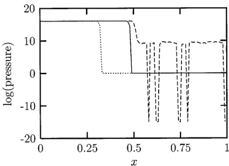
The ability of this ‘‘hybrid’’ code to switch from internal energy to total energy at shock fronts was demonstrated on a variety of one-dimensional test problems. These include the standard Sod shock tube problem with density and pressure ratios of up to 1.0⫻106, and strong standing shocks. Figures 2 and 3 show the results of the most extreme test, a standing shock wave with an upstream Mach number of 1.0⫻108. Results are shown for the hybrid code, a total energy code

共which evolves total energy exclusively兲, and an internal en-ergy code 共which evolves internal energy exclusively兲. The simulations use 100 zones to cover the computational do-main 0⭐x⭐1 and a Courant number of 0.6. The upstream fluid, in the region 0.5⬍x⭐1, has density␳⫽1.0, pressure P⫽1.0, and velocity u⫽⫺1.3⫻108. The downstream fluid, in the region 0⭐x⬍0.5, has density ␳⫽4, pressure P ⫽1.25⫻1016, and velocity u⫽⫺3.2⫻107. Ideally the dis-continuities should be maintained at x⫽0.5. Figures 2 and 3

show the pressure and density after 250 time steps. The CFL condition for this simulation is determined by the upstream velocity, so the upstream fluid travels a distance of ⬃0.006 in each time step.

Figure 2 shows that the total energy code produces ex-tremely large errors in the upstream pressure. As expected, Figs. 2 and 3 show that the results from the internal energy code are quite poor. Altogether, the hybrid code is the most successful at maintaining the proper pressure and density profiles. For this extreme test, the largest errors from the hybrid code appear in the downstream fluid where the den-sity and pressure differ from their ideal values by at most 11% and 1.6%, respectively. The hybrid code also lost about 2.7% of the total energy during the 250-time-step simulation. Because the present code conserves linear momentum, there is no erroneous center of mass motion due to numerical errors. On the other hand, the code does not conserve angular momentum. This is a fairly serious problem because the an-gular motion of the star is the central effect we wish to study. The amount of angular momentum that is lost, or gained, through numerical error is found by computing the total an-FIG. 2. Logarithm of pressure for the strong standing shock test. The curves were obtained from the hybrid code 共solid line兲, total energy code共dashed line兲, and internal energy code共dotted line兲.

gular momentum on the grid, Jgrid, and correcting for the amount of angular momentum that is lost共or gained兲through the grid boundaries, Jlost. The angular momentum passing through the grid boundaries is obtained by computing the angular momentum that moves off the Eulerian grid during each Lagrangian time step. Ideally, the sum of the angular momentum on the grid and the angular momentum lost through the boundaries, Jgrid⫹Jlost, should be constant. As seen in the next section, over the course of the simulation

共8000 time steps兲about 8% of the star’s angular momentum is lost through the boundaries. During this same time, the total angular momentum drops by nearly 25%. Thus numeri-cal errors account for a drop of about 17% in the angular momentum of the star.

In the Newtonian-quadrupole approximation, the gravita-tional wave signal hi j is formed from linear combinations of

components of the second time derivative of the reduced quadrupole moment I–¨i j. The relationship is hi j

⫽(2G/Rc4_{) P}

i j kl_I–¨

kl, where Pi j

kl _{is the projection operator for}

transverse directions and R is the distance from the source to the observation point 关19兴. Using the hydrodynamical equa-tions, the time derivatives that appear in I–¨i j can be

elimi-nated 关20兴so that, to within boundary terms, we have

I–¨i j⫽STF

冕

Here ‘‘STF’’ stands for the symmetric, trace-free part of the expression that follows,viis the fluid velocity,⳵j⫽⳵/⳵xj is

a spatial derivative, and⌽is the gravitational potential. The gravitational-wave signal is computed numerically by using expression 共7兲 for I–¨i j. This calculation is subject to

errors due to the finite size of the computational grid. Recall that during the course of the simulation, matter is expelled from the star. Some of this matter, a total of 0.048M_䉺, passes through the grid boundaries. As a consequence, the relationship hi j⫽(2G/Rc4) Pi j

kl

I–¨kl is not correct, even in the

Newtonian-quadrupole approximation, because the lost mat-ter is not included in the calculation of I–¨_{i j}. A second source of error stems from the fact that boundary terms were dis-carded in the derivation of Eq. 共7兲. These boundary terms would vanish if the density were always zero on the grid boundary. Fortunately, the matter that reaches the boundary has relatively low density and the errors that arise from the missing boundary terms in Eq.共7兲are small. This has been verified by comparing the results from Eq. 共7兲with the re-sults obtained by computing numerically the second time derivative of the reduced quadrupole moment. The numerical derivatives were obtained by performing a least-squares fit to a quadratic using five or seven consecutive data points. The second derivative at the central time is found from the cur-vature of the quadratic. This calculation is subject to a cer-tain amount of numerical noise, but otherwise the results agree quite closely with those obtained from Eq. 共7兲. Since the matter that passes through the grid boundaries does not greatly effect the calculation of I–¨i j with Eq. 共7兲, it is

plau-sible to assume that the errors obtained by equating hi j and

(2G/Rc4) P_{i j}klI–¨_kl are also small.

The frequency spectrum for the gravitational-wave signal is computed with the Lomb normalized periodogram 关16兴. This method was chosen for its ability to handle the un-evenly sampled data. In the Newtonian-quadrupole approxi-mation, the gravitational-wave luminosity is given by L ⫽G I–តi jតI–i j/(5c5), and the radiated energy ⌬E is the time

integral of L 关19兴. The calculation of the time derivative I–

ត_{i j⫽}d I–¨i j/dt must be handled with care since, otherwise,

even small errors in L will accumulate in the integration over time. For this calculation, I use a Savitzky-Golay approach

关16兴. Specifically, the time derivative of the function I–¨i j in

each time interval is computed from the slope of a quadratic polynomial that is obtained from a least-squares fit to several nearest neighbor data points. The number of points used is typically between 10 and 20.

The evolution code was run on a Cray T90 vector com-puter, while the initial data, gravitational wave spectrum, and gravitational wave luminosity were computed on local work-stations. The evolution required 8000 time steps and about 45 CPU hours.

IV. DESCRIPTION OF THE EVOLUTION

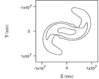
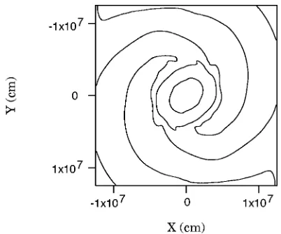
The star retains its predominantly circular, disklike shape for about 10 ms, which amounts to approximately six rota-tion periods for the fluid near the center of the star. Over the next few milliseconds, the bar mode grows rapidly, so that by 13 ms the star is highly elongated as shown in Fig. 4. After a few more milliseconds the central regions of the star recircularize, and by 16 ms the inner density contours have nearly lost their bar shape as seen in Fig. 5. The cycle of bar formation and recircularization repeats; by 19 ms the star again shows a strong barlike shape, as shown in Fig. 6. The episodes of bar formation and recircularization continue with diminishing amplitude and a period of about 6.5 ms. During each episode, the bar undergoes a little more than 1.5 revo-lutions. Near the end of the simulation, at a time of⬃50 ms, the oscillations become quite weak and the star settles into a

bar-shaped configuration of modest strength. See Fig. 7. During the initial episode of rapid bar formation, matter is thrown outward from the ends of the bar. The ejected matter forms long spiral arms, clearly visible in Figs. 4 and 5. Some of this matter is lost off the edge of the computational grid— between 14 and 20 ms the mass loss totals 0.040M_䉺. The subsequent episodes of bar formation are less violent, with only small amounts of ejected mass reaching the grid bound-aries. The mass loss between 20 ms and the end of the simu-lation amounts to 0.008M_䉺.

When the star assumes its bar shape, the individual par-ticles in the inner regions of the star circulate along trajecto-ries that roughly coincide with the constant density contours. For example, at the time shown in Fig. 4, 13.58 ms, the bar is rotating about the center of mass with a period of approxi-mately 4 ms. Individual particles flow along the 1014_g/cm3 density contour with fairly uniform speeds ranging from about 6.5⫻109cm/s to about 7.5⫻109cm/s. The density contour at 1014g/cm3 has a perimeter length of approxi-mately 1.7⫻107cm. Thus the particles orbit along this con-tour with period⬃2.5 ms as the contour precesses about the star’s center with period⬃4 ms.

The shape of the star can be quantified by Fourier

analyz-ing the density in a circle in the equatorial plane关21,12兴. The Fourier coefficients are defined by

Am⫹iBm⫽

1 2␲

冕

2␲

d␸ ␳共␸兲eim␸, 共8兲

where␳(␸) is the density in the equatorial plane at an arbi-trarily chosen distance of 2.0⫻106_{cm from the center of the} star. Here␸is the azimuthal angle. The amplitude of the mth Fourier mode is defined by Cm⫽

冑

2_⫹

B_m2, and the phase angle is ␾m⫽arctan(Bm/Am). Figure 8 shows the natural

logarithm of the ratio of the amplitude C_m and the average density C0 for the m⫽2 bar mode and the m⫽4 mode. The m⫽3 mode is small and is not displayed in Fig. 8. The coefficient C3/C0remains less than 0.01 through most of the evolution, reaching peak values of⬃0.02 in the late stages. The periodic growth and decay of the bar shape is clearly seen in the peaks and valleys of the graph in Fig. 8. The amplitudes grow exponentially for several milliseconds dur-ing the initial episode of bar formation. For the m⫽2 bar mode, the growth rate near 10 ms is d ln C2/dt⬇820/s. For

FIG. 6. Density contours as in Fig. 4, at 19.48 ms.

FIG. 7. Density contours as in Fig. 4, at the end of the simula-tion共52.57 ms兲.

FIG. 8. Natural logarithm of the ratios C2/C0 and C4/C0 of Fourier amplitudes.

the m⫽4 mode, the growth rate is d ln C2/dt⬇1400/s. In polytropic units (␶⫽1.88⫻10⫺5s), the growth rates for the m⫽2 and m⫽4 modes are 0.015 and 0.026, respectively. For m⫽2, this value differs by a few percent from the result 0.0145 reported in Ref.关5兴. In units of the ‘‘dynamical time’’ t_D⫽关R_eq3/(G M )兴1/2_{, where R}

eq is the initial equatorial ra-dius, the growth rates are 0.50/t_D and 0.86/t_D for the m⫽2 and m⫽4 modes. Comparing these results to the values 0.55/t_D and 1.1/t_D obtained from the highest resolution run in Ref. 关3兴, we find a fairly large discrepancy in the m⫽4 case. This difference might be caused by numerical errors in the present code associated with the cartesian grid.

Near the end of the simulation, the oscillations in the Fourier amplitudes have subsided and the star settles into a bar shape with strength C2/C0⬇0.18. The downward drift in C2/C0, visible in Fig. 8, is possibly due to numerical error as discussed below.

The phase angles for the m⫽2 and m⫽4 modes are shown in Fig. 9. The eigenfrequencies are d␾2/dt ⫽3.24/ms and d␾4/dt⫽6.52/ms. The pattern speeds m⫺1d␾m/dt 关12兴 are 1.62/ms for the m⫽2 mode and

1.63/ms for the m⫽4 mode. These speeds, which equal 0.99/tD and 1.0/tD in dynamical time units, agree with the

results obtained in Refs.关5,3兴to within 1%. The approximate equality of the pattern speeds shows that the m⫽4 mode is a harmonic of the m⫽2 bar mode.

The stability parameter ␤ undergoes fluctuations, drop-ping to a local minimum when the bar amplitude C₂/C₀ is a local maximum and rising to a local maximum when the bar amplitude is a local minimum. This behavior is shown in Fig. 10. As the fluctuations diminish, ␤settles to a value of

⬃0.24 with a slight downward drift. Note that this value of␤ is well below the critical value 0.27 for the growth of the bar mode in a constant density star.

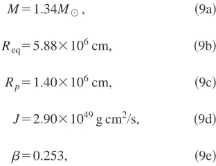
The fact that the bar shape persists with ␤ below 0.27 might indicate that the threshold for bar formation in a ␥ ⫽5/3 star with rotation law given by Eq.共1b兲is actually 0.24 or less. This possibility was tested by evolving a second model star, obtained by modifying the freely specifiable data

in Eq. 共1兲 so that the central value of angular velocity is 3000/s rather than 4000/s. The parameters describing this model are

M⫽1.34M_䉺, 共9a兲

Req⫽5.88⫻106cm, 共9b兲

Rp⫽1.40⫻106cm, 共9c兲

J⫽2.90⫻1049g cm2/s, 共9d兲

␤⫽0.253, 共9e兲

so, in particular, the stability parameter is between 0.24 and 0.27. This model was evolved for approximately 23 ms, which equals about 11 rotation periods for the fluid near the center of the star. During this time, the m⫽2 bar mode showed no signs of growth. We are thus led to conclude that for a ␥⫽5/3 fluid star with rotation law of the type consid-ered here, the dynamical m⫽2 bar mode will not spontane-ously grow unless␤exceeds a critical value near 0.27; how-ever, once a bar shape is established, it can persist for many rotation periods with ␤⫽0.24 or less.

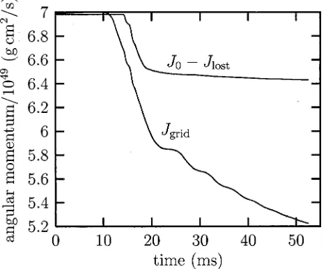
As discussed in the previous section, the numerical code does not conserve angular momentum. In Fig. 11, the total angular momentum on the grid, Jgrid, is plotted as a function of time along with the difference between the initial angular momentum J0⫽6.98⫻1049g cm2/s and the angular momen-tum Jlost that flows off the edge of the numerical grid. Ide-ally, these two curves should coincide; the fact that J_gridfalls below J0⫺Jlostindicates that numerical errors artificially re-move angular momentum from the system. The results for Jlostwere checked by computing the angular momentum flux from each of the saved data sets, which were generated every 50 time steps. The numerically computed time derivative of J_lost is in very close agreement with the angular momentum flux.

I have not yet determined the source of the numerical errors in angular momentum. Note, however, that the errors are not significant until the star begins to develop a notice-able bar shape, at about 10 ms. This suggests that the code has difficulty tracking the leading and trailing edges of the bar-shaped star, with their sharp density gradients, as the bar rotates in the x-y plane.

Since numerical errors cause angular momentum to be lost, it is plausible to expect that rotational kinetic energy is artificially lost as well. This might account for the downward drift in the stability parameter at late times, as seen in Fig. 10. In turn, one might expect a drop in the stability parameter to cause the star’s bar shape to decay. Figure 8 shows that the Fourier amplitude C2is fairly robust at late times with a slight downward trend on average. If angular momentum were not artificially lost, the simulation might show that after the fluctuations cease the bar shape remains unchanged on a dynamical time scale.

V. GRAVITATIONAL WAVES

In the Newtonian-quadrupole approximation, the gravita-tional wave amplitude for the plus polarization state, h_⫹, as measured at a distance R in the equatorial plane of the source, is

c4R

G h⫹共eq兲⫽共cos

2_{␸⫺2兲I–¨}

xx⫹共sin2␸⫺2兲I–¨y y

⫹2 cos␸sin␸I–¨xy. 共10兲

Here, I–¨_{i j} is the second time derivative of the reduced quad-rupole moment and␸is the azimuthal angle of the observa-tion point relative to the 共arbitrary兲 x axis of the source. Figure 12 shows the results for h_⫹ with R⫽20 Mpc and ␸ ⫽␲/2. 共Recent estimates indicate that the distance to the Virgo cluster is⬃20.9 Mpc关22兴.兲In the equatorial plane, the

cross polarization amplitude, h_⫻(eq), is a linear combination of the components I–¨xz and I–¨y z. Since the star is

approxi-mately symmetric under reflections in the equatorial plane, h_⫻(eq) as measured in the equatorial plane is nearly zero.

For an observation point above the north pole of the star, the plus polarization amplitude is

c4R

G h⫹共p兲⫽共2 cos

2_{␸⫺1兲I–¨}

xx⫹共2 sin2␸⫺1兲I–¨y y

⫹4 cos␸sin␸I–¨xy. 共11兲

Since the star is highly flattened and has little motion in the z direction, the zz component of the second time derivative of the unreduced quadrupole moment, I¨zz, is very small.

Fur-thermore, because the shape of the bar does not evolve rap-idly compared to its rotation rate, the xx and yy components satisfy I¨xx⫹I¨y y⬇0. These observations imply I–¨xx⬇⫺I–¨y y.

As a consequence, we see from Eqs. 共10兲 and 共11兲 that h_⫹(p)⬇2h_⫹(eq). This is confirmed by the results of the simulation. As expected, the amplitude h_⫻(p) is almost iden-tical to h_⫹(p), just phase shifted by 45°.

Although the reliability of the results for the gravitational-wave signal is rather poor, due both to the crudeness of the physical model and to numerical errors, it is still of some interest to consider the detectability of these waves. Thus, consider the characteristic amplitude of the source, approxi-mated by关7兴

hc⬇

冉

冊

1/2

. 共12兲

Here ⌬E is the total energy radiated in gravitational waves and fcis the characteristic frequency. The gravitational-wave

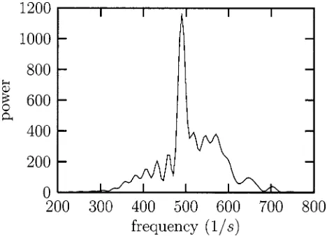
frequency is sharply peaked about 490 Hz, as shown in Fig. 13. The total energy radiated in gravitational waves, as FIG. 11. The angular momentum on the grid, Jgrid, and the

difference J0⫺Jlostbetween the initial angular momentum and the angular momentum lost at the boundaries of the grid.

computed in the Newtonian-quadrupole approximation up to the time the simulation was halted, is ⌬E⬇5⫻10⫺4M_䉺c2. From these data we find the characteristic amplitude of the source to be hc⬇4⫻10⫺22 _{at a distance of 20 Mpc. This} value for hc is a lower bound, since the radiated energy⌬E

will continue to increase as long as the bar persists. Also note that the result hc⬇h

冑

The signal hc⬇4⫻10⫺22is probably too weak to be seen by the first generation of interferometric gravitational-wave detectors, which should have a sensitivity of about 10⫺20 at 500 Hz关6,23兴. The signal might be detectable by the planned advanced detectors, which are expected to have a sensitivity below 10⫺21 at 500 Hz关6,23兴. For a source at a distance of

⬃25 kpc, comparable to the diameter of the Milky Way gal-axy, the characteristic amplitude is hc⬇3⫻10⫺19. This is a relatively large signal that should be detected easily by the first generation of interferometers.

If the simulation is scaled as described in Sec. II, the amplitude as measured at a fixed 共unscaled兲 distance R changes by a factor of␶2/(␮␭2) and the frequency changes by a factor of ␶. For example, with ␭⫽1/2, ␮⫽2, and ␶ ⫽1/4, the amplitude h_⫹(eq) at R⫽20 Mpc is reduced from that shown in Fig. 12 by a factor of 8. The characteristic amplitude hc is also reduced by a factor of 8, to about

5⫻10⫺23at 20 Mpc, and the peak frequency occurs at⬃120 Hz. This signal is somewhat below the expected sensitivity of the advanced gravitational-wave detectors, which is ap-proximately 10⫺22at 120 Hz关6,23兴. At a distance of 25 kpc, the characteristic amplitude is almost 4⫻10⫺20, well above the expected sensitivity of ⬃4⫻10⫺21 _{for the first} genera-tion detectors.

VI. CONCLUSIONS

The simulation presented here shows that a rapidly rotat-ing ␥⫽5/3 fluid star with rotation law Eq. 共1b兲 is dynami-cally unstable to bar formation and that the bar shape, once

established, is relatively long lived. Over the final 10 or 20 ms of the simulation, the star maintains a modest but fairly persistent bar shape with stability parameter␤equal to about 0.24. It is possible that, for ␥⫽5/3 stars with certain initial angular velocity profiles, the threshold for bar formation is actually 0.24 or less. However, further numerical study showed that an axisymmetric star with ␤⫽0.25 initially is stable against growth of the bar mode. Thus, for the models considered here, the dynamical bar mode requires a value of ␤ near 0.27 to grow but the bar shape can persist for many bar-rotation periods with␤⫽0.24 or less. Imamura, Durisen, and Pickett suggest that as long as ␤ is greater than the critical value for growth of the secular instability, about 0.14, a bar-shaped star is dynamically stable against forming an axisymmetric disk 关8兴. The results here are consistent with this conjecture. Recent numerical studies by New, Centrella, and Tohline关3兴also indicate that the bar shape is long lived. The strength of the gravitational-wave signal emitted by an initially axisymmetric, dynamically unstable star depends on the rotating star’s length and time scales. With the nu-merical model scaled to represent a low-density neutron star with soft equation of state, the characteristic amplitude is hc⬇4⫻10⫺22 at a distance of 20 Mpc. With the mo-del scaled to represent a stellar core that has partially col-lapsed and is prevented from contracting to nuclear densities by centrifugal forces, the characteristic amplitude is hc ⬇5⫻10⫺23at 20 Mpc. These signals are probably too weak to be detected by the first generation of interferometers, al-though the neutron star signal might be detectable by the planned advanced interferometers. At a distance of 25 kpc, both signals are quite large and should be detected easily by the first generation interferometers.

ACKNOWLEDGMENTS

I would like to thank John Blondin for helpful discus-sions. Numerical calculations were carried out on the Cray T90 at the North Carolina Supercomputing Center.

APPENDIX

The technique used in this work to solve the equations of hydrostatic equilibrium is similar to the self-consistent field method, first developed by Ostriker and Mark关24兴and later refined by Hachisu 关25兴. The self-consistent field method is based on the integral form of the Euler equation which reads, for the equation of state P⫽K␳␥关24,25兴:

␥K ␥⫺1␳

␥⫺1_{⫹⌿⫹⌽⫽C. 共A1兲}

In this equation,⌿⫽⫺兰dr r␻2 is the ‘‘rotational potential’’ derived from the angular velocity ␻(r), ⌽ is the gravita-tional potential, and C is an integration constant. In the self-consistent field method, one begins with an initial guess for the density ␳, solves the Poisson equation for ⌽, and then uses Eq.共A1兲to obtain a corrected density distribution. The process is then iterated. Typically, the Poisson equation is solved by expanding the potential ⌽ in terms of Legendre FIG. 13. The frequency spectrum of gravitational waves,

polynomials, and the constant C appearing in Eq. 共A1兲 is determined by specifying certain properties at the star’s sur-face. For example, Hachisu fixes the ‘‘axis ratio’’ Rp/Req

关25兴.

For the method used in this paper, the constant C is de-termined by properties at the center of the star. The rotational potential is chosen to vanish at the star’s center, ⌿(0)⫽0, and the constant C is written as

C⫽␥K␳_c␥⫺1⫹⌽c. 共A2兲 Here the subscript c denotes the center of the star. The cen-tral density␳c is specified as input data, along with the

ro-tation law ␻(r). The initial guess for ␳ is chosen to be a static, spherically symmetric polytrope with central density ␳c, obtained by solving numerically the Lane-Emden

equa-tion. The potential⌽and its central value are obtained from the Poisson equation using a multigrid algorithm, as dis-cussed below. Note that with this scheme the center of the star must have nonzero density. This precludes the possibil-ity of generating stars with toroidal surfaces.

Equation共A1兲can be written as F⫽0 where the function F is defined by

F⬅ ␥K ␥⫺1␳

␥⫺1_{⫹⌿⫹⌽⫺C 共A3兲}

and the constant C is given by Eq. 共A2兲. The corrections to the density are obtained from a Newton-Raphson algorithm applied to F⫽0. Note that F(x) is a nonlocal function of ␳(x), where x labels points in space. The nonlocal depen-dence of F(x) on ␳(x) enters through the gravitational po-tential ⌽(x). One might expect that the value of ⌽at the point x is insensitive to the density␳(x) at the same point x, since the potential ⌽is determined primarily by the global properties of the star, such as its mass. With this observation in mind, we compute the variation of F at point x with re-spect to ␳ at point x by dropping the nonlocal terms. This leads to the approximate result ␦F⬇␥K␳␥⫺2␦␳. Then set-ting F⫹␦F⫽0, we find the density correction

␦␳⫽_␥1_K␳2_⫺␥_{共C⫺⌽⫺⌿兲⫺} 1

␥⫺1␳, 共A4兲

to be used for each Newton-Raphson iteration.

I have not constructed a mathematical argument to justify the above assumption, namely, that the nonlocal terms in F

can be ignored in computing ␦F. However, this same as-sumption is implicit in the usual self-consistent field method. As described in Refs. 关24,25兴, for the self-consistent field method the density is updated by solving Eq. 共A1兲 for ␳, ignoring the␳ dependence in⌽. That is, the change in␳is

␦␳⫽

冋

册

⫺␳, 共A5兲

where ⌽ is the solution of the Poisson equation. Formula

共A5兲 can be justified by the same reasoning that led to Eq. 共A4兲, but with the following difference: enthalpy H

⬅␥K␳␥⫺1/(␥⫺1), rather than density ␳, is treated as the independent variable. The variation of F with respect to H, ignoring the ⌽ dependence on H, is ␦F⬇␦H. Setting F⫹␦F⫽0 leads to a new enthalpy distribution H_new ⫽H⫺F. Solving this equation for the new density␳new, we find the density correction ␦␳⫽␳new⫺␳ of Eq.共A5兲.

The initial data code solves the equations of hydrostatic equilibrium at the zone centers of a 513⫻513 grid in the r-z plane of a cylindrical coordinate system. The symmetry axis coincides with the edge of the first column of zones. The density ␳ is computed on the inner 512⫻511 zones. One layer of zones at the top, bottom, and side opposite the sym-metry axis are reserved for setting boundary conditions for the gravitational potential ⌽. The boundary values are ob-tained by expanding the potential in a multipole series that includes monopole and quadrupole terms. 共The dipole and octupole moments vanish due to rotational symmetry and reflection symmery about the equatorial plane.兲The Poisson equation is solved with a multigrid algorithm, adapted from the code described in Ref.关16兴to handle the boundary con-ditions and the cylindrical geometry.

The initial data described in Sec. II was generated by a code that relies on the Newton-Raphson iteration scheme

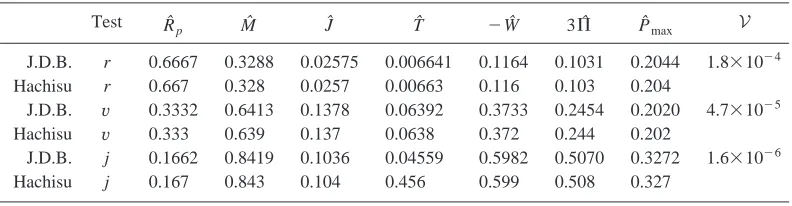
共A4兲and the multigrid Poisson solver described above. The results of three tests of this code共J.D.B.兲are shown in Table I. For comparison, the results obtained by Hachisu 关25兴are also listed. The values reported in the table are scaled as in Hachisu’s self-consistent field method, with Newton’s con-stant G, the equatorial radius Req, and the maximum density ␳max equal to unity. Carets denote these scaled quantities. Also,⌸denotes the volume integral of pressure,兰P dV.

The ‘‘r’’ test assumes a rigid rotation law, ␻(r)⫽␻0, with the scaled angular velocity given by ␻ˆ₀2⫽0.266. The ‘‘v’’ test assumes the ‘‘v-constant’’ rotation law, ␻(r) ⫽v0/

冑

2_{⫽0.215 and dˆ⫽0.100. The ‘‘j’’ test} TABLE I. Comparison of results obtained from the initial data code described here共J.D.B.兲and Hachisu’s

self-consistent field method code.

Test _Rˆ

p Mˆ Jˆ Tˆ ⫺Wˆ 3⌸ˆ Pˆmax V

J.D.B. r 0.6667 0.3288 0.02575 0.006641 0.1164 0.1031 0.2044 1.8⫻10⫺4 Hachisu r 0.667 0.328 0.0257 0.00663 0.116 0.103 0.204

J.D.B. v 0.3332 0.6413 0.1378 0.06392 0.3733 0.2454 0.2020 4.7⫻10⫺5 Hachisu v 0.333 0.639 0.137 0.0638 0.372 0.244 0.202

J.D.B. j 0.1662 0.8419 0.1036 0.04559 0.5982 0.5070 0.3272 1.6⫻10⫺6

assumes the ‘‘j-constant’’ rotation law,␻(r)⫽j0/(d2⫹r2), with jˆ₀2⫽0.0176 and dˆ⫽0.100. For each test, ␥⫽5/3. For Hachisu’s data the virial theorem diagnostic V is typically less than a few times 10⫺4 关25兴. The test results show that the present code and Hachisu’s code differ by less than 1% in every case.

Subsequent testing has shown that the density update in

Eq. 共A4兲is no better, in terms of accuracy and convergence rate, than the usual self-consistent field method update共A5兲. After 30 Newton-Raphson iterations, the results obtained from the two update formulas agree to a few parts in 10⫺9, at worst. For both update formulas, the errors共as compared to the 30-iteration results兲 were at most a few tenths of a per-cent after 10 iterations.

关1兴S. Chandrasekhar, Ellipsoidal Figures of Equilibrium 共Yale University Press, New Haven, CT, 1969兲.

关2兴S. L. Shapiro and S. A. Teukolsky, Black Holes, White Dwarfs, and Neutron Stars共Wiley, New York, 1983兲. 关3兴K. C. B. New, J. M. Centrella, and J. E. Tohline, Phys. Rev. D

62, 064019共2000兲.

关4兴See, for example, R. H. Durisen and J. E. Tohline, in Pro-tostars and Planets II, edited by D. Black and M. Matthews 共University of Arizona Press, Tuscon, 1985兲, pp. 534–575. 关5兴J. Toman, J. N. Imamura, B. J. Pickett, and R. H. Durisen,

Astrophys. J. 497, 370共1998兲.

关6兴See, for example, B. C. Barish, Adv. Space Res. 25, 1165 共2000兲; B. Caron et al., Nucl. Phys. B共Proc. Suppl.兲54B, 167 共1997兲.

关7兴K. S. Thorne, in 300 Years of Gravitation, edited by S. W. Hawking and W. Israel 共Cambridge University Press, Cam-bridge, England, 1987兲, pp. 330–458.

关8兴J. N. Imamura, R. H. Durisen, and B. K. Pickett, Astrophys. J. 528, 946共2000兲.

关9兴J. L. Houser and J. M. Centrella, Phys. Rev. D 54, 7261 共1996兲.

关10兴T. W. Baumgarte, S. L. Shapiro, and M. Shibata, Astrophys. J. Lett. 528, L29共2000兲.

关11兴P. Bodenheimer and J. P. Ostriker, Astrophys. J. 180, 159 共1973兲.

关12兴H. A. Williams and J. E. Tohline, Astrophys. J. 315, 594 共1987兲.

关13兴J. Tassoul, Theory of Rotating Stars 共Princeton University Press, Princeton, 1978兲.

关14兴P. Colella and P. R. Woodward, J. Comput. Phys. 54, 174 共1984兲.

关15兴S. K. Godunov, Mat. Sb. 47, 357共1959兲.

关16兴W. H. Press, S. A. Teukolsky, W. T. Vetterling, and B. P. Flannery, Numerical Recipes 共Cambridge University Press, Cambridge, England, 1992兲.

关17兴G. L. Bryan, M. L. Norman, J. M. Stone, R. Cen, and J. P. Ostriker, Comput. Phys. Commun. 89, 149共1995兲.

关18兴M. Zingale, F. X. Timmes, B. Fryxell, D. Q. Lamb, K. Olson, A. C. Calder, L. J. Dursi, P. Ricker, R. Rosner, P. MacNeice, and H. Tufo, ‘‘Helium Detonations on Neutron Stars.’’ 关19兴C. W. Misner, K. S. Thorne, and J. A. Wheeler, Gravitation

共Freeman, New York, 1973兲.

关20兴L. Blanchet, T. Damour, and G. Scha¨fer, Mon. Not. R. Astron. Soc. 242, 289共1990兲. Similar formulas were obtained by L. S. Finn and C. R. Evans, Astrophys. J. 351, 588共1990兲. 关21兴J. E. Tohline, R. H. Durisen, and M. McCollough, Astrophys.

J. 298, 220共1985兲.

关22兴G. A. Tammann, A. Sandage, and B. Reindl, in Proceedings of the 19th Texas Symposium on Relativistic Astrophysics and Cosmology, Paris, 1998, ‘‘The distance of the Virgo cluster,’’ astro-ph/9904360.

关23兴K. S. Thorne, in Black Holes and Relativistic Stars, edited by R. M. Wald共University of Chicago Press, Chicago, 1998兲. 关24兴J. P. Ostriker and J. W.-K. Mark, Astrophys. J. 151, 1075

共1968兲.