Mechanics of fabric drape

(1)

ABSTRACT

PANDURANGAN, PRADEEP SAMBANDAN. Mechanics of Fabric Drape. (Under the direction of Dr .Jeffrey W. Eischen)

Three dimensional virtual representations of fabrics done based on particle modeling lack accuracy in their representation of various fabrics due to very little understanding of how fabric mechanical properties affect drape.

Particle models represent cloth as a mesh of particles connected by springs. The springs exert forces on the particles causing them to move thus representing the deformation of fabric. The spring constant values input to the simulation correspond to the mechanical properties of the modeled fabric. Fabric mechanical property values obtained from standard testing like the Kawabata evaluation cannot be input directly to the particle modeling software to produce simulations resembling reality. A systematic way of selecting various input parameters to the particle model is developed by comparison of 3D scans of the drape of simple forms of various fabrics to matching simulations produced by the particle model. Since drape is a complex function of many unpredictable variables a simple way of varying only a few parameters in simulations without compromising on their resemblance to reality has been developed.

(2)

The relationship was then tested on more complex apparel and found to produce excellent results.

(3)

MECHANICS OF FABRIC DRAPE

by

Pradeep Pandurangan

A thesis submitted in partial fulfillment of the requirements for the degree of

Master of Science

Department of Mechanical and Aerospace Engineering North Carolina State University

Raleigh, NC July 2003 Approved by:

_____________________________ ___________________________ Dr. Traci May-Plumlee Dr. Eric Klang

____________________________ Dr. Jeffrey Eischen

(4)

BIOGRAPHY

Pradeep Pandurangan was born and brought up in Madras, India. In 2002 he completed his Bachelor of Engineering degree in Mechanical Engineering from The University of Madras, India. He pursued his Masters degree in Mechanical engineering at the North Carolina State University from fall 2002. He worked as a research assistant on a project titled 3D Virtual Draping with Fabric Mechanics and Body Scan Data, sponsored by the National Textile center. He graduated in August 2004.

(5)

ACKNOWLEDGEMENTS

I am immensely grateful to:

• My advisor Dr. Jeffrey Eischen, NC State Department of Mechanical and Aerospace Engineering.

• Dr. Traci May-Plumlee, Technology and Management NC State College of

Textiles.

• Committee member Dr. Eric Klang, NC State Department of Mechanical and Aerospace Engineering.

• Narahari Kenkare, Ph.D. student, Textile Technology and Management, NC

State College of Textiles.

• The National Textile Center, for funding my research through a grant.

• Mike King, David Bruner, and Kim Munro of theTextile Clothing Technology

Corporation.

• Optitex, for donating the Modulate™ simulation software.

• Gadi Zadikoff, ofOptitex R&D.

• My family and friends especially Bharani.

(6)

LIST OF FIGURES

Figure 1.1-Simulation of a garment……….. 1

Figure 1.2-Particle spring grid ………. 3

Figure 1.3- 3D body scanning system………4

Figure 1.4-Simulation done using Modulate™ imported to Geomagic™………… 5

Figure 2.1-Kawabata tensile testing……….. 7

Figure 2.2-Kawabata tensile testing response……… 8

Figure 2.3-Kawabata bending test………. 8

Figure 2.4-Kawabata bending test response……….. 9

Figure 2.5-Kawabata shear test………. 9

Figure 2.6-Kawabata shear testing response………. 10

Figure 3.1-Definition of drape coefficient………. 13

Figure 3.2-Cusick drape meter………... 14

Figure 3.3-Steps in calculation of drape coefficient by scanning and processing in Geomagic™………... 15

Figure 3.4-Measurement of nodes………. 16

Figure 3.5-Drape test setup dimensions………. 16

Figure 3.6-Variation exhibited by fabrics in drape parameters………... 17

Figure 3.7-Pattern used in simulation……… 19

Figure 3.8-Simulation of drape of standard circular specimen………... 19

Figure 3.9-Modulate™ software input parameters………... 20

(10)

Figure 4.1- Tip loaded cantilever beam and particle model of a tip loaded

cantilever beam ……….………... 22

Figure 4.2-Choi and Ko particle model connectivity (shown for center particle)…. 23 Figure 4.3- Formation of initial coordinates of nodes………26

Figure 4.4- Fixed end modeling of cantilever beam with applied tip load………… 26

Figure 4.5-Beam undergoing large deflection……….. 29

Figure 4.6-Tip deflections for a tip loaded cantilever……… 30

Figure 4.7-Tip deflections for a uniformly loaded cantilever……… 30

Figure 4.8 - Particle beam deflections……….. 34

Figure 4.9- Plot of flexural stiffness input to particle model and matching flexural rigidity from theoretical model for tip loading………. 35

Figure 4.10- Plot of flexural stiffness input to particle model and matching flexural rigidity from theoretical model for distributed loading……… 36

Figure 4.11- Non-dimensional plots of flexural rigidity of particle model and matching flexural rigidity from theoretical model for distributed loading……..…. 37

Figure 4.12-Plot of ₂ b WL EI value at saturation against particle load ………... 38

Figure 4.13- Plots of flexural stiffness of particle model and matching flexural rigidity from theoretical model for different resolutions………... 36

Figure 4.14- Non-dimensional plots of flexural stiffness input to particle model and matching flexural rigidity from theoretical model for different resolutions…... 39

Figure 5.1-Scan of drape of circular fabric……… 43

Figure 5.2-Modulate™ simulation satisfying criterion………. 44

(11)

Figure 5.3- KES bending stiffness versus with bending stiffness input to

ModulateTM simulations ………... 45

Figure 5.4-Band of acceptance………... 46

Figure 6.1- Scan of skirt fitted to a mannequin………. 48

Figure 6.2- Scan of a mannequin used for testing………. 48

Figure 6.3-Dimensions of garment1 used in testing………... 49

Figure 6.6-Stages in simulation of garment1………. 51

Figure 6.7-Views of Sateen simulation (blue) and scan (red) of garment1 ……….. 53

Figure 6.8-Views of Lawn simulation (blue) and scan (red) of garment2 ……... 55

Figure 6.9-Views of Momie simulation (blue) and scan (red) of garment3 ……... 56

(12)

LIST OF TABLES

Table 2.1-Bending stiffness and weights of selected fabrics………. 10

Table 2.2-Shearing stiffness and friction coefficient of selected fabrics…………... 11

Table 2.3-Tensile properties of selected fabrics……… 11

Table 3.1-Variation exhibited in drape parameters………... 18

Table 4.1-Results of tip loaded particle model cantilever beam………32

Table 4.2-Results of uniformly loaded particle model cantilever beam……… 33

Table 5.1-Bending stiffness values from matching simulations of fabrics………… 44

Table 6.1-Comparison of scan and simulations of garment1……… 52

(13)

LIST OF SYMBOLS AND ABREVIATIONS

B bending stiffness (dyne-cm) c damping coefficient cm centimeter (10-2m)

DC drape coefficient dyn dyne (10-5Newton) E energy

E Youngs modulus

F, f force

G Shearing stiffness (dyne-cm) g, gm gram

gf gram force (0.009807 Newton) I moment of inertia

Ks, ks stretching spring stiffness Kb, kb bending spring stiffness KES Kawabata evaluation system lp load per particle

L length

LT linearity

Ls stretching spring length Lb bending spring length M, m mass, metre

MIU Surface friction coefficient Np number of particles

P tip load

R,r radius

RT Resilience

t time

UDL uniformly distributed load v velocity

W load per unit length, weight WT tensile energy

κ curvature

δh horizontal deflection

δv vertical deflection t

∆ time step

(14)

1 INTRODUCTION

Accurate 3D virtual representation of fabrics is a very effective tool for the textile industry and would greatly facilitate many aspects of it. At present virtual cloth modeling technologies lack accuracy in their representation of various fabrics. Unless the virtual representations resemble reality they will be of only limited use.

Cloth modeling technologies take into account the nature of the simulated fabric and its surroundings to predict how the fabric might look like virtually. But the mechanics of fabrics is much more complicated than conventional engineering materials like steel because of the complex behavior of cloth and its highly deformable nature. One of the main hurdles towards accurate virtual representations is the lack of understanding of how fabric mechanical properties affect drape. The problem is further complicated by the fact that fabrics exhibit variation in their drape. It was observed in experiments that they do not drape the same way each time.

Figure 1.1- Simulation of a garment

(15)

1.1 Cloth modeling technologies

Cloth materials have distinct properties that make them deform in a different way than other materials. Apart from having a unique behavior each cloth material has its own characteristic way of deforming. A cotton fabric will not deform in the same way as a polyester fabric. Computer simulation of cloth drape has always presented significant problems and has been primarily carried out by a continuum model based on finite elements or a discrete particle based model. There are significant problems with the former continuum based modeling of cloth which assumes the small scale behavior of cloth is simply a scaled down version of its macroscopic behavior. This assumption is not valid for woven, highly deformable, anisotropic and nonlinear cloth. Cloth modeling based on an interacting particle model [1] is based on the microstructure of woven cloth which is not continuous and is a complex microstructure. By representing cloth in a particle model various complexities in the microstructure of cloth are better represented. The particle method is also simpler to implement and needs less computational time. Empirical data from a fabric testing system like Kawabata can provide the required material property input to the simulation system.

In the ideal case test data representing a particular fabric when input to the system should simulate that particular cloth but this is not the case. The fabric test data when input to the simulation system produces simulations which do not accurately represent the cloth leading to ad hoc selection of the input parameters to produce a more accurate simulation. There is a need for a way to systematically select the input parameters in a particle model simulation in order to accurately represent each cloth virtually. This would be of immense value to an apparel designer who could then visualize how a shirt made from different types of fabrics will differ in appearance.

(16)

1.2 Problems associated with cloth modeling

Experience shows that each time a table cloth is draped it hangs in a slightly different manner, the reason being that drape of cloth is governed by a large number of factors which exhibit behavior sensitive to environmental and other conditions. Cloth in itself can be considered as a composite material whose mechanical properties vary with direction. Standard tests like the Kawabata evaluation system only measure average mechanical properties governing cloth deformation because a comprehensive evaluation would be impractical considering time and cost factors. So cloth modeling is typically done with only limited knowledge of the factors influencing drape which leads to lack of realism. Cloth materials are also very diverse structurally. The diversity exhibited structurally should be captured without making any changes to the structure of the modeling technique which makes the predicting drape difficult.

1.3 Cloth modeling using interacting particles

Figure 1.2- Particle spring grid

(17)

represented by energy functions. The total energy of each particle will be the sum of energies due to these interactions plus the gravitational potential energy due to the mass of particles and artificial repulsion energy applied to keep each particle at a minimum distance from others. The total force acting on each mass point can be derived from the energy functions, with the equations of motion of the particle system as the final result. The displacements time history of the particles can be calculated by employing numerically integration (i.e. a time-stepping technique).

1.4 Simulations, scans and their analysis

A brief outline of how the process of generating simulations, scanning of 3D objects and processing the scans and simulations were accomplished is explained below.

Simulations generated using Modulate™ have been used during this research. As mentioned earlier, this software allows users to construct fabric patterns of any desired shape and simulate its drape over an object.

A 3D image of any object can be obtained as a data point cloud by using the 3D body scanner available at the Apparel Design Lab at the NC State College of Textiles, shown in Figure 1.3. The scanner has been extensively used to generate images of the drape of fabrics in order to compare with simulations.

(18)

The simulations generated by Modulate™ and point clouds generated by the scanner were processed by Geomagic™. Geomagic™ is a 3D image processing software system in which surfaces can be generated from point clouds and other analyses such as computation of cross sectional areas and volumes can be done. Figure 1.4 shows a simulation of a garment done using Modulate™ (left) and the same simulation imported into Geomagic™ (right) for analysis.

(19)

2 PROPERTIES INFLUENCING FABRIC DRAPE

2.1 Effect of mechanical properties on drape

Standard fabric testing groups the mechanical properties of cloth into the following categories:

• Tensile

• Bending

• Surface

• Shearing

• Compression

• Weight and thickness

Each fabric has its own distinct set of the above properties and hence it drapes in its own characteristic way. All the parameters mentioned above have an influence on drape and some have a greater effect than others. Hu and Chan [5] have investigated the relationship between fabric drape and mechanical properties derived from standard testing methods. According to their results the following the factors influencing drape, shown in descending order of importance.

Bending>Tensile>Shear>Weight>Surface>Compression

2.2 Measurement of mechanical properties of fabrics by the Kawabata

Evaluation System (KES)

(20)

hysteretic behavior of cloth. This is due to the fact that there is some energy loss during the deformation predominantly due to friction. The testing is done in both the warp and weft directions to account for the anisotropy present in fabrics. Kawabata testing is carried out only in the small deformation regime under an assumption of purely linear elastic behavior. This makes the derivation of various stiffnesses from the plots relatively easy by reducing the data with linear regression and calculating their slopes. The results from the bending, tensile, and shear are described in the sections below.

2.2.1 Tensile properties

During KES tensile testing a load of 500 gf/cm is applied along the width direction of the specimen shown in Figure 2.1. The strain along the width direction is minimal. The strain rate is kept at a constant of ₄_×₁₀−3_{/sec. A curve as shown in Figure 2.2 is obtained}

Figure 2.1- Kawabata tensile testing The characteristic values extracted from the curves are

• LT : Linearity

• WT : Tensile energy per unit area (gf.cm/cm2)

• RT : Resilience (%) LT =

max max

2

ε ×

F WT

WT =

∫

max

0

ε

Fd (gf.cm/cm2₎

RT =

_WT

d F

∫

max

0 '

ε

x100 (%)

F

5cm _20cm

(21)

Figure 2.2- Kawabata tensile testing response

2.2.2 Bending property

During the KES bending test pure bending is imposed on the fabric sample in a range of curvatures of −2.5≤ ≤κ 2.5cm-1 with a constant rate of curvature change of 0.5 cm-1/sec enforced. The bending rigidity B is obtained as the slope of the moment curvature curve shown in Figure 2.4. The average of the slopes in the warp and weft directions is given as the bending rigidity.

Figure 2.3- Kawabata bending test 20cm 1cm

M F, gf/cm

500 Fmax

(22)

Figure 2.4- Kawabata bending test response

2.2.3 Shearing property

The KES shear test is done as shown in Figure 2.5 with a constant tension W of 10gf/cm applied along the direction orthogonal to the shearing force. The shear stiffness G is taken as the slope of the Fs-Φ plot shown in Figure 2.6. The mean slope is measured between .5o_{and 5}o_{and the average of warp and weft directions is taken as G.}

Figure 2.5- Kawabata shear test 20cm

5cm Shear testing

Φ

Fs W

M, (gf-cm)/cm

K, 1/cm

(23)

Figure 2.6- Kawabata shear testing response

2.3 Kawabata test results

Kawabata tests were done on 16 fabrics including both woven and knit structures. The results of the testing are summarized in the tables below. The compression test on the fabrics was not done because of the expected negligible influence on drape.

Fabric Bending stiffness, _{B (dyne-cm)} Weights ,W (g/m2)

Plain1 35 110

Interlock 6 38 202

Rib 38 211

Lawn 68 95

Plain 2 82 194

Challis 91 153

Twill 1 122 190

Plain 4 129 168

Oxford 5 129 211

Sheeting 138 189

Sateen 180 248

Poly Twill 213 254

Corduroy 251 217

Momie 470 180

Twill 3 551 292

Plain20 580 256

Table 2.1- Bending stiffness and weights of selected fabrics Shearing property Fs, gf/cm

Φ, degree

(24)

Fabric Shear stiffness, G gf/(cm-degree)

Surface friction coefficient,

MIU

Plain1 1.110 0.210

Interlock 6 0.552 0.288

Rib 0.9489 0.30

Lawn 1.8117 0.24

Plain 2 2.297 0.161

Challis 0.7412 0.26

Twill 1 2.060 0.200

Plain 4 2.634 0.219

Oxford 5 2.093 0.188

Sheeting 2.3055 0.23

Sateen 4.4332 0.22

Poly Twill 0.7929 0.37

Corduroy 2.4607 0.23 Momie 3.0817 0.28

Twill 3 6.045 0.248

Plain20 4.3681 0.19 Table 2.2- Shearing stiffness and friction coefficient of selected fabrics

Fabric LT _(gf-cm/cmWT 2₎ RT (%)

Plain1 0.570 11.700 49.270 Interlock 6 0.779 3.394 45.573

Rib 1.7127 12.7014 47.4833

Lawn 0.6532 13.1004 52.6073

Plain 2 0.631 13.120 47.430

Challis 0.6198 14.8874 50.8424

Twill 1 0.660 6.710 58.540

Plain 4 0.696 11.308 44.174

Oxford 5 0.658 6.561 52.122

Sheeting 0.6184 26.5521 36.9171 Sateen 0.6881 11.6228 49.4988 Poly Twill 0.6194 37.3918 66.7362

Corduroy 0.5916 19.094 50.6522

Momie 0.7043 12.0568 58.0024

Twill 3 0.775 8.200 52.787

(25)

2.4 Problems associated with the KES

The mechanical properties of cloth are roughly divided into three regions: the initial resistance region, region of low deformation, and a region of high deformation. The mechanical behavior of cloth throughout the region of deformation is non-linear. It is only in the region of low deformation that the mechanical properties follow a reasonably regular pattern and can be represented by a linear mathematical model. The data obtained from the KES only represent the mechanical properties of cloth in the low deformation regions and this severely limits the accuracy with which one can relate the measured mechanical properties to the input constants in the 3D simulations where large deformations are expected and present.

(26)

3 DRAPE OF CIRCULAR FABRIC PARTS

3.1 Measurement of fabric drape

Fabric drape is defined as the extent to which fabric will deform when it is allowed to hang under its own weight. Fabrics have different weights and different mechanical properties like bending stiffness, stretching stiffness, etc. This causes each fabric to deform in its own characteristic way.

The most fundamental method for quantifying drape and one which is widely used in the textile industry is the measurement of the drape coefficient [7]. The drape coefficient is measured on an initially horizontal annular ring of fabric. A single number is obtained for the drape coefficient with a theoretical maximum of 100 and a theoretical minimum of 0. A solid circular fabric specimen is allowed to drape over a circular horizontally placed rigid disc with the center of the fabric coinciding with the center of the disc. Thus, an annular ring of fabric is allowed to drape over the disc and typically the fabric deforms into a series of folds around the disc. The drape coefficient is defined as the ratio of the total area of the annular ring obtained by vertically projecting the shadow of the draped specimen to the undeformed pre-drape area (expressed as a percentage).

Figure 3.1- Definition of drape coefficient

The drape coefficient is conventionally measured by an apparatus called the Cusick drape meter shown in Figure 3.2 in which the circular piece of fabric is supported horizontally by an inner circular disc and an outer annular disc. During the drape test cloth is placed over the two discs and the outer annulus is lowered gradually while the

R r

(27)

Figure 3.2- Cusick drape meter

An alternative method of measuring the drape coefficient was accomplished by using the 3D body scanner in the NC State College of Textiles Design Lab. The circular piece of cloth was draped over the circular disc and scanned. The scan data is obtained as a point cloud which is then processed using the Geomagic™ software. The drape coefficient and other useful drape parameters can then be extracted from the processed scan. The steps in the calculation of drape coefficient from a 3D scan of the draped fabric are shown in the figures below.

(28)

(c) (d)

(e) (f)

Drape coefficient = 100 2 1

×

A A

Figure 3.3- Steps in the calculation of the drape coefficient by scanning and processing in Geomagic™

While measuring the drape coefficient the fabric drapes in regular smooth folds called nodes. The characteristic dimensions of these nodes were also measured as shown in Figure 3.4.

(29)

Figure 3.4- Measurement of nodes

3.2 Variability exhibited in fabric drape

Fabrics do not drape the same way each time. By studying the range of variation exhibited in the actual fabric drapes one can get an idea of how close a simulation must be in order for it to pass as an acceptable virtual representation of the respective cloth.

Drape measurement was carried out on 36cm diameter fabric samples draped on an 18cm diameter disc (see Figure 3.5). Each fabric was draped 12 times, 6 times on the front side and on the 6 times on the back side (the front and back sides of the cloth can be distinguished based on the weave of the cloth), in the Cusick drape meter as well as in the 3D scanner. In each trial the drape coefficient, number of nodes, and the nodal dimensions were recorded. As expected each fabric exhibited a wide range of variation in the drape parameters.

Figure 3.5- Drape test setup dimensions

The figures below show the variation exhibited in the number of nodes, drape coefficients, node dimensions during the 12 trials.

d2

d1 _d 3

Node

18cm

9cm

(30)

0 1 2 3 4 5 6 7 8 9

0 10 20 30 40 50 60 70 80 90

0 20 40 60 80 100 120 140 160 180 200

Figure 3.6- Variation exhibited by fabrics in drape parameters during variability tests

d1 d2 d3

Plain1 Interlock6 Rib Lawn Plain 2 Challis Twill1 Plain 4 Oxford 5 PolyTwill Corduroy Momie Twill 3 Plain20

Dimensions of nodes

(mm

)

Dra

pe coefficient

(31)

3.3 Accurate representation of a fabric

In order to simulate the appearance fabric drape virtually, one has to know what an accurate representation of a fabric is. Fabric drapes exhibit a fairly wide range of variation as the experimental results showed in the previous section. The variation exhibited in the drape parameters is summarized below.

Fabric DC Number

of

nodes d1(mm) d2(mm) d3(mm) Plain1 27-36 6,7 98-110 51-67 60-67 Interlock6 27-38 6,7 89-125 42-60 60-67 Rib 15-21 6,7,8 71-95 42-65 45-57 Lawn 43-54 6,7 101-130 35-58 70-75 Plain 2 46-63 6,7 104-150 38-65 67-75 Challis 26-34 6,7,8 79-94 41-57 55-64 Twill1 42-51 5,6,7 111-154 40-71 68-77 Plain 4 46-63 6,7 107-148 31-52 71-79 Oxford 5 42-63 5,6,7 120-165 31-62 74-83 Poly twill 35-40 6,7 88-112 45-65 61-70 Corduroy 67-75 5,6,7 120-171 26-50 76-85

Momie 77-83 5,6 151-186 30-50 81-87 Twill 3 70-83 5,6 141-180 32-47 73-80 Plain20 73-85 5,7 132-185 28-52 76-87

Table 3.1- Variation exhibited in drape parameters

Looking at the wide variation in drape exhibited by fabrics it is understood that there is no one target value for a simulation to match for it to be accepted as a good match to the actual fabric. Instead if a simulation falls within a wide region of acceptance it could pass as a good match to the actual drape.

3.4 Circular fabric part simulation using Modulate™

(32)

diameter 36cm used in Modulate™ simulations and Figure 3.9 shows stages in the simulation of the drape of the circular fabric part.

Figure 3.7- Pattern used in simulation

(33)

3.5 Factors influencing drape in particle model simulations

Even though particle model simulations are based on the woven microstructure of cloth it doesn’t represent the full thread structure of the woven cloth. Due to the inability of particle model simulations to exactly represent woven cloth materials some of the mechanical properties influencing the drape of real fabric mentioned previously do not influence the particle model simulations in the same way and to the same extent as they do the drape of a real fabric.

Particle model simulations (using Modulate™) do not take into account certain factors like shear and bending hysteresis which do have an effect on the drape of the real fabric. Another drawback is that cloth by nature is not isotropic and hence doesn’t produce a symmetric drape about an axis of symmetry. Modulate™ simulations do not capture these effects. Only the stretching stiffness parameter is directionally dependent. There is only a single bending stiffness parameter, same for shear. A picture of the Modulate™ cloth parameter input window is shown in Figure 3.10.

Figure 3.9- Modulate™ software input parameters

(34)

(35)

4 TWO DIMENSIONAL PARTICLE MODEL

4.1 Introduction

In this section an approach based on theory is made to determine how various spring constants that are input to the particle model formulation affect drape shapes. A 2D version of the Choi and Ko [2] particle model was programmed. A cantilever beam was selected as a model configuration because a theoretical solution is available in the large deflection regime. Figure 4.1 shows a tip loaded cantilever beam (above) and the corresponding particle model idealization (below). By comparing the deflections of the particle model with those of the theoretical model a relationship can be obtained between the constants input to the particle model and those of the theoretical model.

Figure 4.1- Tip loaded cantilever beam (above), particle model of the tip loaded cantilever beam (below).

4.2 Choi and Ko particle model

The Choi and Ko model provides the theoretical basis for the Modulate™ software. Problems relating to stability and realism presented previously in the particle model were overcome by Choi and Ko in their model [2]. In this model two types of particle interaction are involved and are referred to as type1 and type2 (see Figure 4.2). The type1 interaction represented by red lines is responsible for stretch and shear resistance. Such

x y

p1 p2 pi-1 pi+1

P

pi xi yi y

P

(36)

connections are referred as sequential connections as they connect every particle to all of its neighboring particles. The type2 interaction represented by the blue lines is responsible for bending and compression resistance. Such connections are referred to as interlaced connections and they connect each particle to particles immediately adjacent to all of its neighboring particles (i.e. the adjacent particle is skipped).

Figure 4.2- Choi and Ko particle model connectivity (shown for center particle alone)

4.3 Particle Method Formulation

4.3.1 Forces acting on particles

Each particle is subject to two types of forces generated by interaction with neighboring particles. Stretching forces are generated between neighboring particles (sequential), while bending and compression forces are generated between every other particle (interlacing).

4.3.2 Type 1 or stretching interaction

(37)

(

)

s ij s ij s ij s

L

x

L

x

L

x

k

E

≤

=

≥

−

=

0

2

1

2

wherexij =xj −xi, 

     = i i i y x

x and

        = j j j y x

x , Ls is the natural length of the spring

(distance between the neighboring particles) and ks is the stretching spring stiffness. The

force acting on particle ‘i’ due to the stretching deformation is then given by.

(

)

L

x

L

x

L

x

k

x

E

f

ij ij ij ij s ij s i i

≤

=

≥

−

=

∂

−

=

0

4.3.3 Type 2 or bending interaction

This interaction takes place between every other particle. Choi and Ko have approximated the bent equilibrium shape of a buckled beam as a circular arc (constant curvature) and the corresponding bending energy as.

2 2 1 _κ b bL k E =

where Lb is the natural length of the bend element, while kb is the flexural spring

stiffness. The curvature κ can then be calculated given the distance between the end points of the particles and the natural length of the bend element,

1 2 sinc ij b b x L L κ ₌ − _ _     where sinc(x) x x) sin( = .

Approximate formula for computation of curvature:

(38)

        − ≈ b ij b L x L 6 1

2

κ

The above formula for curvature was derived from the exact expression for curvature as follows. 1 2 sinc ij b b x L L κ₌ −       sinc 2 ij b b x L L κ  _{ =}     b ij b b L x L L = 2 2 sin κ κ

Performing a two term Taylor series expansion of the left hand side of the above equation, b ij b L x L = × −           2 3 2 1 2 κ

Solving for κ ,

        − = b ij b L x L 6 1

2

κ

The above formula for κ is simple to compute and produces κ values that are within approximately 5% of the exact solution for0.75≤ ≤1

b ij L x

.

The force acting on particle ‘i’ due to the bending deformation is then given by

1 2 cos sinc

2 2 ij b b b i ij x L L k x

f κ κ κ

− −      = _ _ _ _ __       4.4 Programming

(39)

1. A mesh of particles is numbered and the coordinates of each particle is recorded. Element lengths can then be computed. The elements are identified as being either type 1 or type 2.

Figure 4.3- Formation of initial coordinates of nodes

2. The motion of the first two particles is constrained in order to force the model to behave like a cantilever beam (left end zero transverse deflection and slope). The picture shows a concentrated tip load applied, but a distributed load can also be treated.

Figure 4.4- Fixed end modeling of cantilever beam with applied tip load

3. The effective force acting on each particle is the sum of internal forces fi for type 1 and

type 2 interactions, damping forces and any externally applied forces.

damping spring

external f f

f

F = + +

or

v c f

f f

F

bend stretch

external + + +

=

P

x y

y

x pi

p1 p2

Ls Ls

2 Type1 elements

1 Type 2 element

(40)

Where                     ⋅ ⋅ = 2 2 1 1 y x y x v v v v

v , is the vector of particle velocities and c is a damping coefficient.

4. The equations of motion that are to be solved are v dt x d = F M dt v

d ₌ −1

Where M is a diagonal mass matrix with each diagonal element being the particle mass,

                            ⋅ ⋅ = p N p N y x y x y x x 2 2 1 1

is the vector of particle positions

and Np is the number of particles in the model.

(41)

The differential equations to be solved are:

( )

t x k v dt x d , = =

(

t x v

)

l F M dt v d , , 1 ₌ − = Runge-Kutta iteration:

( )

(

)

(

)

(

)

(

)

(

)

t a x x b b b b b a a a a a t b v t a x t t l b t b v t a x t t k a t b v t a x t t l b t b v t a x t t k a t b v t a x t t l b t b v t a x t t k a v x t l b x t k a ∆ + = + + + = + + + = ∆ + ∆ + ∆ + = ∆ + ∆ + ∆ + =       ∆ + ∆ + ∆ + =       ₊∆ ₊ ∆ ₊ ∆ =       ₊∆ ₊ ∆ ₊ ∆ =       ∆ + ∆ + ∆ + = = = 4 3 2 1 4 3 2 1 3 3 4 3 3 4 2 2 3 2 2 3 1 1 2 1 1 2 1 1 2 2 6 1 2 2 6 1 , , , , 2 , 2 , 2 2 , 2 , 2 2 , 2 , 2 2 , 2 , 2 , , ,

Where ∆t is the time step.

4.5 Tip deflections from large deflection beam theory

The exact differential equation to be solved while calculating the deflection of beams is given by.

(42)

Where the quantity ds dθ

represents the curvature of the beam. When the deflection is

small the quantity ds dθ

is approximated by ₂

2

dx v d

. This approximation is satisfactory provided the slopes of the beam are small. When the slopes and hence the deflections become large the exact differential equation of the deflection curve must be used.

Figure 4.5- Cantilever beam undergoing large deflection

Non-dimensional curves of the tip deflections of a cantilever beam acted upon by a concentrated tip load P or a uniformly distributed load of W, load per unit length are given in Figures 4.6 and 4.7, respectively (from references [3] and [4]). The flexural rigidity of the beam is denotedEI.

y

L

δv

δh dθ

ρ

ds

P x

x dx

(43)

Figure 4.6- Tip deflections for a tip loaded cantilever

Figure 4.7- Tip deflections for a uniformly loaded cantilever 0 5 10 15 20 25 30 35 40 45 50 -0.2

0 0.2 0.4 0.6 0.8 1 1.2

L

h

δ

L

v

δ

EI PL2

0 100 200 300 400 500 600 0

0.1 0.2 0.3 0.4 0.5 0.6 0.7 0.8 0.9 1

L

−

δ

h

L

v

δ

(44)

4.6 Required data input

The program requires the following constants to be input. 1. Length of stretch elements, Ls

2. Length of bend elements, Lb 3. Length of beam, L

4. Stretch spring stiffness, ks 5. Flexural spring stiffness, kb 6. Number of particles, Np

7. Tip load, P or load per particle, lp

8. Particle mass, m 9. Damping coefficient, c 10. Time step, ∆t

4.7 Results

The tip deflection was computed using the particle model approach for a fixed set of constants and the flexural rigidity. Then the flexural rigidity required for the theoretical beam model to produce the same deflections under the same load was determined. The vertical tip deflection of the two models was matched. It was observed that the horizontal deflections of the particle and theoretical model were within 5% of each other. Cloth materials are characterized by high stiffness to stretching. This behavior has been modeled by using high values of stretching spring constant (ks) compared to the bending spring constant (kb) in the particle model. Furthermore the deflections of the particle model are not very sensitive to variations in the stretch constant, hence the effect of varying the spring constant in the following simulations is insignificant and ignored.

(45)

Input Data Results Deflections from particle

model Case P

(N) ks (N-mm) kb (N-mm2)

Ls (mm)

Lb

(mm) Np

δh

(mm) (mm)δv

Matching flexural rigidity from beam theory (N-mm2)

1. .03 -1.23 -2.26 .028

2. .05 -.88 -1.95 .049

3. .075 -.77 -1.81 .06

4. .1 -.74 -1.77 .063

5. 1 -.73 -1.76 .064

6.

-.02

3 -.62 -1.66 .072

7. .03 -1.77 -2.57 .021

8. .05 -1.41 -2.36 .044

9. .075 -1.16 -2.17 .068

10. .1 -1.07 -2.07 .081

11. 1 -1 -2 .091

12.

-.04

400

3

.5 1 6

-.95 -1.97 .095

13. .75 1.5 4 -.87 -1.94 .25

14. .5 1 6 -1.63 -2.4 .1

15. .375 .75 8 -2 -2.59 .049

16.

-.1 200 1

.3 .6 10 -2.26 -2.69 .028

17. .75 1.5 4 -1.17 -2.17 .35

18. .5 1 6 -1.6 -2.49 .15

19. .375 .75 8 -2.2 -2.68 .06

20.

-.2 200 1

.3 .6 10 -2.42 -2.76 .035

(46)

Input Data Results Deflections from particle model Case p l Particle Load (N) ks (N-mm) kb (N-mm2)

Ls

(mm) (mm)Lb Np

δh (mm) δv (mm) Matching flexural rigidity from beam theory (N-mm2)

1. .01 -1.99 -2.72 .005

2. .02 -1.46 -2.46 .013

3. .03 -1.1 -2.2 .023

4. .05 -.77 -1.87 .036

5. .075 -.65 -1.71 .042

6. .1 -.62 -1.66 .045

7.

-.005 400

1

.5 1 6

-.57 -1.62 .047

8. .01 -2.29 -2.83 .004

9. .02 -1.88 -2.67 .01

10. .03 -1.55 -2.5 .02

11. .05 -1.14 -2.21 .035

12. .075 -.92 -2 .048

13. .1 -.82 -1.88 .056

14.

-.008 400

1

.5 1 6

-.75 -1.81 .061

15. -.1 2 4 4 -1.07 -3.78 5.54

16. -.067 1.33 2.67 6 -2.34 -5.15 3.14

17. -.05 1 2 8 -3.89 -6.19 1.74

18. -.04 .8 1.6 10 -4.83 -6.69 1.1

19. -.0333

1000 10

.67 1.33 12 -5.54 -7 .74

20. -.15 2 4 4 -1.6 -4.58 6.04

21. -.1 1.33 2.67 6 -2.74 -5.49 3.98

22. -.075 1 2 8 -4.42 -6.44 2.1

23. -.06 .8 1.6 10 -5.37 -6.88 1.31

24. -.05

1000 10

(47)

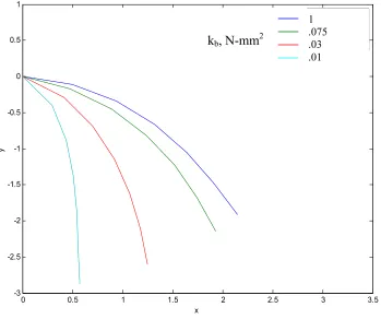
Figure 4.8 shows the deflections of the uniformly loaded particle model beam for different values of flexural spring stiffness while keeping other constants the same.

0 0.5 1 1.5 2 2.5 3 3.5

-3 -2.5 -2 -1.5 -1 -0.5 0 0.5 1

x

y

Kb = 1 Kb = .075 Kb = .03 Kb = .01

Figure 4.8-Deflections of the 2D particle beam for different values of bend spring constant, other inputs Np = 6, l_p = -.01 N, ks = 400 N/mm, Ls = .5mm, Lb = 1mm,

L = 3mm, c = 1 Nsec/mm, m = 1g.

Figures 4.9 and 4.10 are plots of flexural stiffness input to the particle model and the matching flexural rigidity values from beam theory. The plot shows a generally bi-linear relationship between these variables.

1 .075 .03 .01

(48)

0 0.5 1 1.5 2 2.5 3 0.02 0.03 0.04 0.05 0.06 0.07 0.08 0.09 0.1

Kb input to the particle model

C or re sp on di ng fl ex ur al r ig id ity fr om th e th eo re tic al m od el

load = -.02 load = -.04

Figure 4.9-Plot of flexural stiffness input to particle model and matching flexural rigidity from theoretical model for tip loading

0 0.1 0.2 0.3 0.4 0.5 0.6 0.7 0.8 0.9 1

0 0.05 0.1 0.15 0.2 0.25

C orre sp ond in g f le xu ral ri gi di ty f rom t he th eoret ic al m ode l

load/particle = -.005 load/particle = -.008 load/particle =-.01 load/particle = -.02 load/particle = -.1

Figure 4.10-Plot of flexural stiffness input to particle model and matching flexural rigidity from theoretical model for distributed loading

N

(49)

The above plots have two distinct regions. Region1 (region of the curves with high slope) is where there is significant variation in deflection with variation in the kb

value input to the particle model. This region is called the “Response region”. Region2 (region of lesser slope) is where increase in kb doesn’t produce significant variation in

deflection. This region is referred to as the “Saturation region”. The response region becomes longer with increase in load and has a slightly less slope when compared to the response region of a curve of lesser load. As cloth materials have very less bending rigidity, the response region encompassing low values of flexural stiffness corresponds to real cloth behavior.

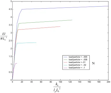
Figure 4.11 shows dimensionless plots of flexural stiffness input to particle model and matching flexural rigidity from theoretical model for distributed loading

0 20 40 60 80 100 120 140 160 180 200 0

0.5 1 1.5 2 2.5 3 3.5 4 4.5 5

load/particle = -.005 load/particle = -.008 load/particle =-.01 load/particle = -.02 load/particle = -.1

Figure 4.11-Non dimensional plots of flexural rigidity of particle model and matching flexural rigidity from theoretical model for distributed loading

3

b

WL EI

2

b p

b L l

k

(50)

The above non-dimensional curves show that the response region is linear and the difference in slopes of the response region caused by variation in load is minimal even though the ratio of highest and lowest load values used is 20

005 .

1 . ₌

− −

= . The ratio of weight per unit area for a heavy and light weight fabric is unlikely to be as high as 20 and would realistically be about 4. Hence the differences in slopes of response region in the above non dimensional plots caused by variation in load can be ignored for fabrics. Therefore all fabrics have a common and linear response region. The saturation region branches off from a common response region and it varies significantly for each load. A plot of

3 b WL

EI

value at saturation against lp is shown below. From this plot the point at

which saturation occurs for each loading can be determined.

0 0.01 0.02 0.03 0.04 0.05 0.06 0.07 0.08 0.09 0.1

1 1.5 2 2.5 3 3.5 4 4.5 5

Figure 4.12-Plot of ₂ b WL

EI

value at saturation against lp

lp

3 b

WL EI _at

saturation

(51)

Simulations with varied element sizes showed that the overall stiffness of the beam decreases with decrease in element size or increase in number of particles. Figure 4.13 is a plot of flexural stiffness input to the particle model and matching flexural rigidity from theoretical model of a beam of same loading and spring constants but with different particle resolutions.

0 0.1 0.2 0.3 0.4 0.5 0.6 0.7 0.8 0.9 1

0 0.01 0.02 0.03 0.04 0.05 0.06 0.07 0.08 0.09 0.1

C or re spo nd in g f le xur al r igi di ty f rom t he t he or et ic al m ode l

UDL = -.12

Np = 6 Np = 8 Np = 12

Figure 4.13-Plots of flexural stiffness of particle model and matching flexural rigidity from theoretical model for different resolutions

(52)

0 50 100 150 200 250 300 350 400 0

0.5 1 1.5 2 2.5

Np = 6 Np = 8 Np = 12

Figure 4.14-Non-dimensional plots of flexural stiffness input to particle model and matching flexural rigidity from theoretical model for different resolutions

4.8 Determination of flexural stiffness from fabric testing

The flexural rigidity of cloth and its weight can be determined from testing methods such as FAST and Kawabata. The weight of the cloth corresponds to the load to be applied in the particle model. The non-dimensional plot of flexural stiffness input to the particle model as a function of the experimentally determined flexural rigidity can be determined by performing a few simulations and following the steps given below.

• The slope of the common response region is determined for a selected particle model resolution.

• The point of branching of the saturation region can be determined from plots of non-dimensional flexural rigidity values at saturation against load per particle. The non-dimensional plots of flexural stiffness input to the particle model and matching flexural rigidity from theoretical model is not affected by different

2

b

WL EI

2

b p

b L l

(53)

(54)

5 RELATIONSHIP BETWEEN MEASURED FABRIC

MECHANICAL PROPERTIES AND INPUT

PARAMETERS TO PARTICLE MODEL

SIMULATIONS

The goal of this thesis was to find a relationship between fabric mechanical properties obtained from standard testing and those input to Modulate™ simulations. The development of such a relationship was based on generating simulations and comparing them with the real fabric drape shapes based on several objective criterion. The following section describes the generation of such a relationship using the testing done with the circular forms.

5.2 Criterion for acceptance of a simulation of circular fabric

The proposed relationship between fabric mechanical properties and those input to Modulate™ simulations was developed by comparing the drape of circular parts of real fabric with those of simulations. There was a need to define criteria to classify a simulation as a good match to reality or not. The repeatability tests have shown that fabrics exhibit wide variation in drape shape. Based on results from the repeatability tests the criterions for accepting a simulation as an acceptable match to the actual drape of a fabric were defined as.

• The drape coefficient of the simulation should be within ±10% of the mean value obtained from the repeatability tests.

• The number of nodes in the simulation should be equal to the number of nodes obtained in any one of the 12 trials done for each fabric.

• The dimensions of the nodes (d1, d2, d3) of the simulation should be within

20

(55)

5.3 Generation of simulations satisfying criterions

Simulations satisfying the criterions were performed with the following input parameters. Parameter Value Units

• Bending stiffness : Variable dyne-cm

• Stretching stiffness : X=1500,Y=1000 g/cm

• Shear stiffness : 300 dyne-cm

• Friction coefficient : .25

• Resolution : 1.5 cm

• Weight : variable, from KES g/m2

The values for the stretching and shear stiffness were selected arbitrarily at the above values. The constants were fixed so that all the tested fabrics could be successfully simulated. It must be noted that the fabrics selected for testing encompass a wide spectrum of properties and the simulation input parameters must be a reasonable fit for the fabrics lying in the extremes. For example Lawn weighs 95 g/m2 while Twill3 weighs 292 g/m2. The stretching and shear stiffness were selected such that there were not any problems simulating both these fabrics. Furthermore as mentioned previously in section 2.4, the KES tensile test data doesn’t accurately give an idea of how stiff a fabric really is.

The reason for imparting a different stretching stiffness in one direction than the other is to impart some degree of anisotropy like real cloth so that the simulations don’t look exactly symmetric about a plane of symmetry.

However, the friction coefficient is the average of the measured values for all the fabrics. The friction coefficients of the fabrics do not vary very much from their mean and their influence on particle model simulations is minimal. A mesh resolution of 1.5 cm was chosen as it was discovered that anything greater than that value will be too coarse for a circular fabric of diameter 36cm.

(56)

Generation of simulations satisfying the proposed criterions is illustrated with an example case presented below.

Figure 5.1- Scan of drape of circular fabric Parameters associated with the scan shown in Figure 5.1:

• Name : Oxford

• Mean DC from repeatability tests : 52

• Number of nodes obtained during tests : 5,6,7

• Mean value of d1 : 142 mm

(57)

Input parameters to simulation:

• Bending stiffness : 8000 dyne-cm

• Weight : 211 g/m2

Parameters associated with the simulation:

• DC : 57 (within ±10% of mean DC)

• Number of nodes : 5 (matches nodes in scan)

• d1 : 154 mm (within ±20% of the mean value)

Since the simulation satisfies the three criterions it is classified as acceptable. Table 5.1 shows the bending stiffness input to simulations to produce simulations satisfying the criterions for other fabrics.

Fabric

KES Bending stiffness (dyne-cm)

Bending stiffness for simulations (dyne-cm) Plain1 35.574 1500 Interlock6 38.02 2000

Rib 38.12 1500 Lawn 68.404 2500 Plain 2 82.222 5000

Challis 91.82 4500 Twill1 122.206 6000 Plain 4 129.262 7000 Oxford 5 129.262 8000 PolyTwill 213.15 5000 Corduroy 251.174 15000 Momie 470.204 20000 Twill 3 551.152 26000 Plain20 580.74 23000

(58)

5.4 Relationship developed from testing of circular form

A significant amount of data was generated by testing the drape of circular forms of different fabrics. The KES tests were also performed on all those fabrics. Simulations were also generated matching each of the tested fabrics. A relationship was then developed by putting together all the gathered data. Figure 5.3 shows a number of points fit to a straight line. Each of those points corresponds to a fabric. The bending stiffness input into the simulations for matching simulations of each fabric was plotted against the KES bending stiffness. Other parameters relevant to the plot are.

• Weight : from KES g/m2

0 5000 10000 15000 20000 25000 30000

0 100 200 300 400 500 600 700

Bending stiffness from KES (dyne-cm)

B endi ng s ti ff n es s i nput i n to M odul at e si m u la ti o n s (d yn e-cm )

(59)

5.5 Band of acceptance

The criterions for comparison mentioned in section 5.2 allow a ±10% variation of DC of the simulation from that of the mean value of scans, a ±20% variation in the dimensions of nodes, and a variation in the number of nodes. Each of the data points in Figure 5.2 corresponds to one simulation of each fabric that satisfies the criterions. But many other simulations for each fabric with a different input bending stiffness can be produced satisfying the criterions. Therefore each data point can be shifted up or down and hence the line of best fit obtained above can be allowed to shift up or down by a reasonable value. In other words the line of best fit should be made into a band of acceptance.

For example, taking ±10% from the mean value (12500 dyne-cm) of bending stiffness input into Modulate™ simulations as the allowance we get ±1250 dyne-cm as an allowance. Figure 5.4 shows this allowance as a band of acceptance.

0 5000 10000 15000 20000 25000 30000

0 100 200 300 400 500 600 700

Bending stiffness from KES (dyne-cm)

B endi ng s ti ff n es s i nput i n to M odul at e si m u la ti o n s (d yn e-cm )

Figure 5.4- Band of acceptance

(60)

6 TESTING ON GARMENTS

In the previous chapter a relationship was developed between fabric mechanical properties and those input to Modulate™ simulations for the standard circular form. Any such relationship will be useful only if it holds well on apparel pieces of irregular shape. This chapter presents details of testing the validity of the previously obtained relationship on garments. The testing was done with apparel which was expected to give the most variation in drape with variation in mechanical properties.

6.2 Factors affecting drape of garments

The most important factors influencing drape of garments are as follows [9]:

• The type of fabric-woven, knitted, or satin

• The cut and construction of garment-alignment of warp and weft directions

• Treatment of fabric during manufacturing

• Amount of friction present when it contacts itself or surroundings

• Extra weights due to hems

• Pleats, tucks, gathers, padding, pressing, steaming

6.3 Drape of a garment

(61)

Figure 6.1- Scan of a skirt fitted to a mannequin

6.4 Details of testing

The stiffness relationship was tested by scanning garments fitted to mannequins, running simulations of garments of the same dimension fitted to the scan of the mannequin used in the testing, and comparing them based on criterions. The simulations were input with parameters derived from the previously obtained relationship between measured bending stiffness and the optimal stiffness used for simulation. Skirts and gowns of different fabrics and dimensions were made and tested on two mannequins of different dimensions.

(62)

As it is obvious from the Figures 6.3, 6.4, and 6.5 the garments were constructed with a minimal number of seams to reduce the influence of such. Other factors which could influence drape such as pressing, hemming etc were avoided. The garments were always constructed with the warp direction along the long (vertical) direction.

Figure 6.3- Dimensions of garment1 used in testing (all dimensions in cm)

(63)

Figure 6.5- Dimensions of garment3 used in testing (all dimensions in cm)

The pictures below show snapshots of the simulation of garment1.

(64)

(c)

Figure 6.6- Stages in simulation of garment1

6.5 Metrics and criterions used for comparison

Two factors were used in the comparison of scans and simulations of garments.

• The volume occupied by closing the top and bottom of the garment- this is analogous to DC of circular tests.

• The number of folds obtained in the bottom section- this is analogous to number of nodes of circular tests.

The criterions used for classifying a simulation as an acceptable match to reality were developed taking into account the wide range of variation that fabrics exhibit in their drape and were defined as follows.

• The volume occupied by the simulated garment should be within ±15% of the volume occupied by the scan of the garment.

• The number of nodes obtained in the simulated garment should be within ±2 of the number of nodes obtained in the scan of the garment.

6.6 Results of testing

(65)

of the scan and simulation of the example case put together and shows details of the scan. It also shows the input parameters used to produce the simulation.

6.6.1Garment1

SCAN SIMULATION Fabric Target

number of nodes

Target volumes

(cm3)

Number of nodes obtained

Volumes obtained

(cm3)

% difference

between target and

actual volumes Lawn 7 65338 6 73000 11.7 Challis 7 61614 6 72111 17

Plain 2 6 65655 6 73063 11.2

Twill1 6 68875 6 76903 11.6

Plain 4 6 68137 6 77937 14.4

Oxford 5 5 79327 6 76477 -3.5

Sateen 5 70378 5 73559 4.5 PolyTwill 5 67468 6 77183 14.3 Corduroy 6 69940 5 77333 10.5 Momie 5 80934 5 78423 -3.1

Twill 3 6 68875 5 70124 1.8

Table 6.1- Comparison of scan and simulations of garment1 Selected fabric for example case : Sateen

Scan:

• Volume : 70378 cm3

• Number of nodes : 5

Simulation:

• Number of nodes : 5 Input parameters:

(66)

(67)

6.6.2Garment2

number of nodes

Target volumes

(cm3)

Volumes obtained

(cm3)

% difference

between target and

actual volumes

Lawn 7 65008 6 65064 0.09

Challis 7 61509 6 60242 -2.06

Plain 2 8 65428 6 64238 -1.82

Twill1 7 63933 5 67553 5.66

Plain 4 6 68630 6 66508 -3.09

Oxford 5 7 65276 5 67801 3.87

Sateen 5 70840 5 73338 3.53

Corduroy 7 65820 5 74378 13.00

Momie 5 68858 5 76481 11.07

Twill 3 7 67173 5 70380 4.77

Table 6.2- Comparison of scan and simulations of garment2 Selected fabric for example case : Lawn

Scan:

• Number of nodes : 7 Simulation:

(68)

Figure 6.8- Views of Lawn fabric simulation (blue) and scan (red) for garment2

6.6.3 Garment3

number of nodes

Target volumes

(cm3)

Volumes obtained

(cm3)

% difference

between target and

actual volumes

Lawn 3 88805 3 92385 4.03

Momie 3 93126 3 99815 7.18

Table 5.3-Comparison of scan and simulations of garment3 Selected fabric for example case : Momie

Scan:

(69)

Simulation:

(70)

6.7 Conclusions

All the simulations done can be classified as acceptable matches to the scans based on developed criterions. In most cases the simulations fall well within the region of acceptance lending credence to the validity of the relationship on garments.

Mechanics of fabric drape

ABSTRACT

MECHANICS OF FABRIC DRAPE

BIOGRAPHY

ACKNOWLEDGEMENTS

TABLE OF CONTENTS

LIST OF FIGURES

LIST OF TABLES

LIST OF SYMBOLS AND ABREVIATIONS

1 INTRODUCTION

2

PROPERTIES INFLUENCING FABRIC DRAPE

∫

WT

∫

3

DRAPE OF CIRCULAR FABRIC PARTS

4

TWO DIMENSIONAL PARTICLE MODEL

(

)

L

x

L

x

L

x

k

E

≤

=

≥

−

=

0

2

1

(

)

L

x

L

x

x

x

L

x

k

x

E

f

≤

=

≥

−

=

∂

∂

−

=

0

( )

(

)

( )

(

)

(

)

(

)

(

)

(

)

L

δ

L

δ

L

_WT