Improved Streamflow in Adaptive Reservoir Operation.

of Dr. Sankar Arumugam and Dr. Ranji S Ranjithan).

The main focus of this study is to improve short-term streamflow forecasts and to utilize them in adaptive reservoir operation to enhance sustainability. A combination scheme is developed to integrate reforecasts from a numerical weather model and disaggregated climate forecasts from ECHAM4.5 for developing 15-day ahead precipitation forecasts. Evaluation of the weather-climate information (WCI) based biweekly forecasts under leave-five out cross-validation shows that WCI based forecasts perform better than reforecasts in many grid points over the continental United States. WCI forecasts perform particularly better during summer months when reforecasts have a limited skill. Even though the disaggregated climate forecasts do not perform well at many grid points, the primary reason WCI based forecasts perform better than reforecasts is due to the reduction of the overconfidence of reforecasts. Since the Disaggregated Forecasts (DF) are better dispersed than Reforecasts (RF), combining them with reforecasts results in improved 15-day ahead precipitation forecasts. Improved precipitation and streamflow can be used for adaptive management of water resources system, e.g., reservoir operation.

by Hui Wang

A dissertation submitted to the Graduate Faculty of North Carolina State University

in partial fulfillment of the requirements for the degree of

Doctor of Philosophy Civil Engineering

Raleigh, North Carolina 2012

APPROVED BY:

_______________________________ ______________________________

Dr. Sankar Arumugam Dr. Ranji S Ranjithan

Committee chair Committee co-hair

________________________________ ________________________________

DEDICATION

BIOGRAPHY

ACKNOWLEDGMENTS

The author thanks to his committee members for providing scientific guidance and mentoring during the graduate study at North Carolina State University. They are Dr. Sankar Arumugam, Dr. Ranji Ranjithan, Dr. Downey Brill and Dr. Anantha Aiyyer. What the author learned from his professors through group meetings and one-to-one research discussions are far more than technical approaches to solve the scientific problems studied in this dissertation, but also the general philosophy of carrying independent research.

The author is in debt to Dr. Kenneth W. Harrison for his mentoring all the time. Sincere appreciation goes to Dr. Zheng Fang and Dr. Qing Shao at Wuhan University. The author appreciates his officemates in Mann 319A, Mann 425 and Daniel’s Hall for the wonderful time we spent together.

TABLE OF CONTENTS

LIST OF TABLES... vii

LIST OF FIGURES ... viii

Chapter 1 Motivation and Introduction... 1

Chapter 2 Integration of Climate and Weather Information for Improving 15-day Ahead Accumulated Precipitation Forecasts... 6

2. 1 Introduction ... 6

2.2 Datasets ... 10

2.3 Methodology ... 14

2.3.1 Temporal Disaggregation ... 14

2.3.2 Combination Scheme... 16

2.4 Results and Analysis ... 19

2.5 Discussion ... 27

2.6 Summary and Conclusions... 33

Chapter 3 A Framework for Incorporating Ecological Releases in Sustainable Reservoir Operation... 34

3.1 Introduction ... 34

3.2 Methodology ... 38

3.2.1 Framework Description ... 38

3.2.2 Mathematical Formulation of Reservoir Operation... 43

3.3 Illustrative Study ... 53

3.3.1 Site Description ... 53

3.3.2 Result Analysis ... 55

3.3.3 Tradeoff Analysis ... 62

3.5 Conclusion... 67

Chapter 4 The Value of Ensemble Streamflow Forecasts in Sustainable Reservoir Operation... 72

4.1 Introduction ... 72

4.2 Reservoir Operation With Synthetic ESP ... 75

4.2.1 Synthetic ESP Generation ... 75

4. 2.2 Reservoir Operation Optimization Model ... 78

4.3 Results and Discussion... 85

4.3.1 Value of Improved Streamflow Forecasts ... 85

4. 3.2 Value of Streamflow Forecasts Updating... 89

4.4 Summary ... 92

Chapter 5 Summary and Conclusion ... 94

REFERENCES ... 99

APPENDICES ... 111

LIST OF TABLES

Table 2.1: Performance of the 15-day ahead precipitation forecasts obtained from the combination of weather and climate information (WCI) expressed as the number of grid points exhibiting RPSS > 0 for the first fifteen days (RPSS1) and the second fifteen days

(RPSS2). ...25

Table 3.1: Objectives that are optimized and constrained in each scenario. ..…….……….52

Table 3.2: Comparison of the number of mis-hits for the alterations in the six flow parameters due to current operation. …….………...………..58

Table 4.1:Comparison of monthly hydropower generation, end-of-month storage failure rate and total mis-hits for all the scenarios investigated in this study. The average values and the standard deviation (in parenthesis) are based on the 30 random trials for each simulated scenario. ………...86

Table 4.2: Comparison of monthly mis-hits in each ecological parameter for releases resulting from different skills for a single realization of ESP. ………...………88

LIST OF FIGURES

Figure 2.1: Schematic diagram of the combination approach………9

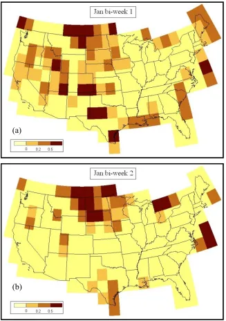
Figure 2.2: MSSS between disaggregated ECHAM4.5 precipitation forecasts and the reforecasts for the first fifteen days (a) and the second fifteen days (b) in January. MSSS>0 indicates MSE of disaggregated biweekly forecasts is lesser than the MSE of the reforecasts indicating potential for the proposed combination scheme (Figure 1). ……….……….13

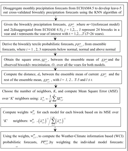
Figure 2.3: Flowchart of the combination algorithm described in section 3.2…….18

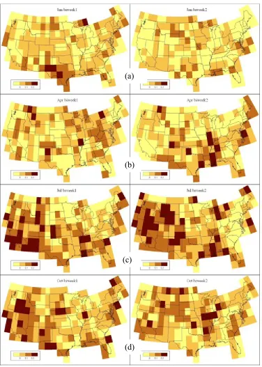
Figure 2.4: RPSS of WCI based forecasts over reforecasts with the left (right) column indicating the first (second) fifteen days for the selected months over four seasons: (a) January; (b) April; (c) July; (d) October……….…….21

Figure 2.5: Comparison of RPS between reforecast and WCI based forecasts for all months. Panel (a) represents pooled RPS (180 X 26) for the first fifteen days and panel (b) is pooled RPS for the second fifteen days. Solid (Dashed) boxplots represent the RPS of reforecasts (WCI based forecasts). ………..23

(dotted) box-plots are for grid points with both RPSS1 and RPSS2 greater (less) than 0. The

box-plot on the left (right) represents for disaggregated ECHAM 4.5 (reforecast model). …26

Figure 2.7: Best model for one month under each season over the continental United States based on RPS. SM1 denotes disaggregated ECHAM4.5 forecasts, SM2 denotes the reforecasts and WCI denotes weather-climate combination forecasts………....29

Figure 2.8: Number of grid points under which each forecasts (SM1, SM2, WCI) during biweek 1 (a) and biweek 2(b) have the lowest RPS for each month over the continental United States. ………..30

Figure 2.9: Box-plots of dispersion parameter,, of the disaggregated GCM forecasts (solid box) and reforecast (dotted box) in the proposed combination scheme for different months: (a) January; (b) April; (c) July; (d) October. Dispersion parameters are grouped in such a way with RPSS1 and RPSS2 of WCI being greater than and lesser than 0. ………...32

Figure 3.1: An adaptive framework of reservoir operation. ..…………...……….41

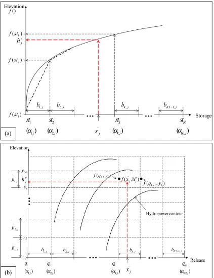
Figure 3.2: (a) Linearization for the storage-elevation curve; (b) Two-dimensional linearization for hydropower generation. ………...……….50

Figure 3.3:Optimization models of different scenarios investigated in this study..………53

Figure 3.5: Alterations in monthly mean flow under current operation: (a) shows the shift in October mean flow between pre-impact and post-impact years; (b) presents the number of mis-hits in the three categories (low, medium, and high) for mean flow in each month. ………...……….……..57

Figure 3.6: Total number of mis-hits for the four scenarios (A, B, C, and D) and current operation………..…59

Figure 3.7:The daily reservoir releases in Oct 1964 for current operation and Scenario B for O c t o b e r , 1 9 6 4 … … … . . . … … 6 1

Figure 3.8:Monthly hydropower generation for Scenarios A (solid box-plots) and D (dashed box-plots). ………...………. 62

Figure 3.9: (a) The tradeoff between hydropower generation and monthly water supply ratio for Scenarios E and F. (b) Monthly hydropower generation for Scenario E.………. 64

Figure 3.10: Correlation between monthly average flow and 1-day minimum flow over pre-impact years. ………...66

Figure 4.1: An Illustrative example of synthetic ESP with skill indicator r_{being 0.7 (a) and} 0.5(b). ………..……77

Figure 4.3: (a) Schematic illustration for coupling method A: Daily ESP with a certain skill is used to determine the daily releases for the entire month; (b) Schematic illustration for coupling method B: Daily ESP available at T0 is used to decide the first 15 day releases while

updated ESP is employed to determine the releases for the rest of the month………....84

Figure 4.4:Comparison of hydropower generation for two ensemble streamflow predictions with different skill levels; solid box-plots are for skill level r=0.9, and the dotted box-plots are for r=0.5………...86

Figure 4.5: (a) Comparison of daily releases in October 1950 for one realization of the synthetic ESPs with different skills; (b) Comparison of October mean release between pre-impact and post-pre-impact years for the three different synthetic ESPs. ………87

Figure 4.6:Comparison of mis-hits, for all six ecological flow parameters, among different scenarios investigated. …….……..……….89

Figure 4.7: (a) Updated releases for the last two weeks in October, 1950 based on a representative realization of ESP. (b) Comparison of the total number of mis-hits between updated ESP and non-updated ESP for one realization………...…………...…….91

Chapter 1 Motivation and Introduction

purposes. Recent studies in the literature (e.g., Shiau and Wu, 2004; Suen and Eheart, 2006; Yang and Cai, in press) suggest incorporating hydrological flow alteration as an evaluation tool in reservoir operations. Most of these studies focus on finding a release pattern using historical data. This can be improved, however, by employing an adaptive release policy based on reservoir inflow.

sustainable reservoir operation is described with an illustration using a hydropower reservoir in Virginia. In Chapter 4, improved streamflow forecasts from Chapter 2 are coupled with the proposed reservoir operation framework from Chapter 3 to illustrate the value of improved streamflow forecasts, as well as the value of streamflow forecasts updating. In Chapter 5, the research findings from this dissertation are summarized and future research directions to extend current study are outlined.

The study presented in Chapter 2 employs model combination approach to integrate weather and climate models for improving 15-day ahead accumulative precipitation forecasts. A combination algorithm is proposed to integrate Disaggregated Forecasts (DF) from ECHAM 4.5 and Reforecasts (RF) numerical weather model to obtain a Weather-Climate Information (WCI) based forecasts. The performance of WCI-based model is evaluated over the continental United States. Analyses of the ensemble forecasts of the combination approach reveal that the primary reason WCI-based forecasts perform better than RF is due to the reduction of the overconfidence of reforecasts. Improved medium precipitation forecasts can be used to improve streamflow forecasting skill.

including releases for water supply, irrigation and hydropower generation are modeled as a mixed integer linear programming problem. Hydropower generation, which is represented by a nonlinear function that usually depends on head and flow, is linearized using a two-dimensional approximation. Investigations using a reservoir in Virginia demonstrate that compared to standard releases based on current operation practice, releases simulated using this adaptive framework perform better in mimicking pre-development flows. Tradeoff among the multiple uses and ecological releases is also investigated. In addition, perfect streamflow forecasts are used to examine whether the proposed approach can effectively balance anthropogenic uses and ecological flow requirements.

Chapter 2 Integration of Climate and Weather Information for

Improving 15-day Ahead Accumulated Precipitation Forecasts

2. 1 Introduction

initial conditions. Ensemble forecasting techniques have also been pursued to account for uncertainties in initial conditions resulting in improved forecast reliability. Various approaches have been investigated for recalibration of weather forecasts that use the ensemble mean (Wilks and Hamill, 2007) as well as the moments of the forecast probability distribution functions (PDFs) (Wilks and Hamill, 2007; Hamill et al., 2004).

forecasting skill than any individual model and can even outperform the single best model if single models are overconfident.

The main intent of this chapter is to improve medium range precipitation forecasts by combining 15-day ahead precipitation forecasts from reforecast dataset (Hamill et al., 2006) and disaggregated forecasts from one-month ahead precipitation forecasts from ECHAM 4.5 (Li and Goddard, 2005). As shown in the schematic diagram (Figure 2.1), we first disaggregate one-month ahead precipitation forecasts from GCM to obtain 15-day precipitation forecasts. Then, combine the disaggregated precipitation forecasts with 15-day ahead precipitation forecasts from weather models based on the proposed combination scheme. Thus, the objectives of this study are to: (1) develop a combination scheme that uses weather and climate forecasts to improve 15-day ahead accumulated precipitation forecasts; (2) examine the circumstances that make the combination reliable; and (3) investigate why the combination scheme results in improved predictions.

Figure 2.1:Schematic diagram of the combination approach to improve medium-range weather forecasts

GCM (ECHAM 4.5) monthly precipitation forecasts (Li and

Goddard, 2005)

Reforecast model (Hamill et al., 2006)

Combination scheme Disaggregated 15-day

precipitation forecasts

This chapter is organized as follows: Section 2 provides detailed information on weather and climate forecasts used in the study along with the motivation behind the proposed combination. The combination algorithm and the disaggregation approach are presented in detail in Section 3. Section 4 discusses results by evaluating the 15-day ahead precipitation forecasts from the combination scheme and also investigates the basis behind the improved performance of the combination scheme. Finally, we conclude with the salient findings arising from the study.

2.2 Datasets

This study employs three datasets for developing WCI-based precipitation forecasts: (a) 15-day ahead precipitation forecasts from numerical weather forecasting model (Hamill et al., 2006); (b) one-month ahead precipitation forecasts from ECHAM 4.5 (Li and Goddard, 2005) and (c) gridded observed daily precipitation for evaluating the developed forecasts

(http://iridl.ldeo.columbia.edu/SOURCES/.NOAA/.NCEP/.CPC/.REGIONAL/.US_Mexico/.

daily/).

of NOAA (http://www.esrl.noaa.gov/psd/forecasts/reforecast/data.html ). For this study, we consider the 15-day accumulated precipitation forecasts issued on the 1st day and 15th day of the month for developing the WCI precipitation forecasts.

Climate Forecasts: For climate forecasts, we consider one-month ahead retrospective precipitation forecasts from ECHAM 4.5 (Roeckner et al. 1996) forced with constructed analogue SSTs (Li and Goddard, 2005). These retrospective forecasts are available for seven months-ahead with the forecasts being updated every month from January 1957 (http://iridl.ldeo.columbia.edu/SOURCES/.IRI/.FD/.ECHAM4p5/.Forecast/.ca_sst/.ensemble 24/.MONTHLY/.prec/). We disaggregated the one-month-ahead forecasts into two biweekly precipitation forecasts using the K-Nearest Neighbor (K-NN) disaggregation algorithm of Prairie et al. (2007) (discussed in Section 3.1).

precipitation forecasts and observations. This resulted in two candidate biweekly forecasts, disaggregated ECHAM 4.5 forecasts and reforecasts, for developing the weather-climate information combined forecasts. Both the combination scheme and the skill measures for all the forecasts were calculated based on the anomalous biweekly time series of precipitation forecasts and observations.

An initial investigation was carried out to examine the potential benefits in combining disaggregated climate forecasts and weather forecasts. One-month ahead precipitation forecasts from ECHAM 4.5 were disaggregated using the K-NN algorithm proposed by Prairie et al. (2007), and compared with the retrospective 15-day ahead precipitation forecasts from reforecast model. For a given month, we consider two forecasts with one from day 1 to day 15 and another from day 16 to the end of month. For a given grid point, mean square error (MSE) over 26 years (1979-2004) were calculated for both forecasts. MSE for a given forecast is computed by averaging the squared error between the observed biweekly precipitation (Ot) and the ensemble mean of the given forecast (Pt). The

performance of both forecasts was compared using Mean Square Skill Score (MSSS) (Equation 1) with MSEc and MSEw denoting disaggregated climate forecasts and weather

reforecasts, respectively.

 1 c w MSE MSSS

based on MSSS for the first fifteen days (Figure 2.2a) and the second fifteen days (Figure 2.2b) clearly shows that for various grid points, particularly over upper Midwest,

Figure 2.2: MSSS between disaggregated ECHAM4.5 precipitation forecasts and the reforecasts for the first fifteen days (a) and the second fifteen days (b) in January. MSSS>0

(a)

indicates MSE of disaggregated biweekly forecasts is lesser than the MSE of the reforecasts indicating potential for the proposed combination scheme (Figure 1).

disaggregated ECHAM 4.5 forecasts have lower MSE values than those of reforecast model. This indicates that a proper combination of disaggregated climate forecasts and weather forecasts could result in improved medium-range forecasts. The next section discusses the methodology for obtaining WCI-based forecasts over the continental United States.

2.3 Methodology

In this section, we briefly describe the disaggregation methodology by Prairie et al. (2007) and the proposed scheme for combining weather and climate forecasts.

2.3.1 Temporal Disaggregation

Various stochastic parametric models have been developed for disaggregation. Linear stochastic framework was originally developed by Valencia and Schaake (1973), which was modified by Grygier and Stedinger (1990) to obtain improved parameter estimates. Compared to parametric methods, non-parametric approach has gained more attention for its simplicity and successful application in many hydrological problems (Lall, 1995). The advantage of the non-parametric approach in disaggregation was demonstrated in kernel-based approach by Tarboton et al. (1998). A robust and simple approach kernel-based on resampling is proposed to achieve space-time disaggregation (Prairie et al., 2007) to avoid kernel density fitting. Recent works on streamflow disaggregation based on nonparametric approach have shown improvements over traditional parametric schemes (Tarboton et al., 1998; Kumar et al., 2000; Robertson et al., 2004; Lee et al., 2010). In this study, we apply nonparametric disaggregation of Prairie et al. (2007) to disaggregate one-month ahead precipitation forecasts from ECHAM 4.5 to biweekly precipitation forecasts. Daily observed precipitation is summed up from the 1stday to the 15thday and 16thday to the 30thday. We did not include the daily precipitation on the 31st day of relevant months (January, March, May, July, August, October and December). For February, we considered the second forecasting period from the 16thday to the end of the month.

monthly precipitation by computing the Euclidean distance from the conditioning variable (i.e., ECHAM4.5 forecasts) to the observed monthly precipitation. The observed biweekly precipitation for the respective neighbors was resampled to constitute ‘N’ ensembles of biweekly disaggregated forecasts. The number of ensembles (w(k)*N) that each identified neighbor represents in the conditional PDF (i.e., represented by ‘N’ ensembles) is estimated by the kernel weighting function (Equation 2.2) suggested by Lall and Sharma (1995).

1

1 ( )

1

K

k

w k k

k  



where

w k

( )

Leave-five-out cross-validated disaggregated forecasts showed reduced MSE for all the months (figure not shown) for K=10 to 12 neighbors. Thus, temporal disaggregation from monthly precipitation to 15-day accumulated precipitation was carried out independently over each grid point for all months by selecting ‘K=10’ neighbors under leave-five out cross-validation. A total of 100 ensemble members of 15-day accumulated precipitation were produced to generate probabilistic biweekly precipitation forecasts.

2.3.2 Combination Scheme

model issued on the 1stand 16thday of the month and disaggregated biweekly forecasts from ECHAM 4.5 monthly precipitation forecasts. The essence of the combination scheme is to assign weights to each one of the candidate forecasts according to their performance in historical years over the same forecasting period. First, ensembles of both candidate forecasts were converted into tercile probabilities, _{, ,}m

i j t

PP ,(i=1,2,3 denoting the below-normal, normal and above-normal categories, respectively) based on the 33rd and 67th percentiles of the observed precipitation. We then evaluated the skill of the two candidate models by computing the squared error m_,

j t

SE between the observed precipitation and the conditional mean of the forecasts for all the years from 1979-2004. Then, both the forecasts available for the period 1979-2004 were combined in a leave-five-out cross validation mode. For instance, to develop combined biweekly forecasts for the 1st two weeks of June in the year 1986 (j = 13th biweek in the year), we computed the distance dl between the ensemble mean of the

current forecast _EP13,1985m _{and the rest of the forecasts} 13,

m t

EP (t≠1986 and four additional years). Based on the distance (dl), we selected ‘K’ neighbors and computed the mean square error

13,1986

m _{over ‘K’ neighbors (selection of ‘K’ is discussed below). Based on the MSEvalue, the}

weight for an individual model was calculated as:

Figure 2.3: Flowchart of the combination algorithm described in Section 2.3.2. Given the biweekly precipitation forecasts, m_,

j t

EP ,where m=1(reforecast model)

and 2(disaggregated from ECHAM 4.5), j = 1,2,.., J represent 24 biweeks in a year andtrepresents the year of interest with t = 1,2,..,T(T=26 years).

Compute the distance, dl, between the ensemble mean of current EP_{j t}m_, and the

rest of the ensemble mean, m_, j l EP

, with l = 1, 2... T-5and l≠ t.

Compute weights wm_{j t,} for each model for each biweek based on its MSE over ‘K’ neighbors: wm_{j t,} =

 

 

1 1

, ,

1

M

m m

j t j t m

   





Using the weights,wm_{j t,} , to compute the Weather-Climate information based (WCI) probabilistic forecasts, _{, ,}wci

i j t

PP ,by weighting the individual model forecasts:

M



Disaggregate monthly precipitation forecasts from ECHAM4.5 to develop leave-5 out cross-validated biweekly precipitation forecasts using the KNN algorithm of Prairie et al. (2007)

Obtain the square error, m_, j t

SE , between the ensemble mean of m_, j t

EP and the observed biweekly precipitation, Oj, over all the years for both models.

Choose the number of neighbors, K, and compute Mean Square Error (MSE)

over ‘K’ neighbors using: _{, ,}

1

1 K

m m

j t j l

l SE K   



Derive the biweekly tercile probabilistic forecasts, _{, ,}m i j t

where 13,1986

m

w represents the weight of model mfor the 1stbiweek in June for the year 1986.

Once the weights were obtained for both the candidate models, a weighted average of the tercile forecasts were calculated to obtain the weather-climate information combined biweekly tercile forecasts. To find the optimum ‘K’ value, we repeated the same procedure (Figure 2.3) and chose the ‘K’ neighbors that resulted in the best skill for the WCI-based forecasts for the selected biweek at a given grid point. The optimum number of neighbors ‘K’ was found to be 10-15 depending on the biweek (not shown). The skill measure that we employed for selecting the ‘K’ neighbors based on leave-five out cross-validation is the average Rank Probability Score (RPS), which computes the mean squared error between the tercile probabilities and the observed category that is represented as 1 (Wilks, 1995). A detailed description of all the steps of the combination scheme is provided in Figure 3. Using this approach, we developed an integrated biweekly precipitation forecasts derived from weather and climate forecasts over the period 1979-2005. The next section presents a detailed evaluation of the skill of the WCI-based biweekly forecasts.

2.4 Results and Analysis

forecasts (reforecasts) outperforms the reforecasts (WCI forecasts). The RPSS value represents how much of the RPS has been reduced (RPSS > 0) or increased (RPSS < 0) compared to the reference forecasts, which we consider as the reforecasts.

Figure 2.4: RPSS of WCI based forecasts over reforecasts with the left (right) column indicating the first (second) fifteen days for the selected months over four seasons: (a) January; (b) April; (c) July; (d) October.

(a)

(b)

(c)

R

PS

R

PS

(a)

(b)

This is partly due to the relatively poor performance of the reforecast model in summer season (Clark et al., 2004; Hamill et al., 2008). The improvement of the WCI-based forecasts compared to the single reforecast model reveals that there is utility in using disaggregated climate forecasts in improving the 15-day ahead forecasts. Disaggregated climate forecasts utilize the ensemble mean of the climate forecasts and the observed structure of the biweekly precipitation under similar monthly totals to develop biweekly forecasts.

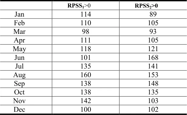
Table 2.1 summarizes the total number of grids in which WCI forecasts outperform the reforecast model (i.e., RPSS > 0). RPSS1 and RPSS2 denote the RPSS for biweek 1 and

biweek 2, respectively. From Table 1, March seems to be the month with lowest total number of grid points exhibiting positive RPSS values: 98 (93) for 1st (2nd) fifteen days. The performance of WCI forecasts improves substantially during the spring season, but WCI forecasts perform much better than the reforecasts during the summer season. RPSS1 is

positive for 160 out of the 180 grid points and RPSS2 is positive for 153 grid points in

season (results not shown). We examine the contribution of reforecasts and disaggregated forecasts to the combination scheme by analyzing the weights estimated in the combination scheme.

Table 2.1: Performance of the 15-day ahead precipitation forecasts obtained from the combination of weather and climate information (WCI) expressed as the number of grid points exhibiting RPSS > 0 for the first fifteen days (RPSS1) and the second fifteen days

(RPSS2).

RPSS1>0 RPSS2>0

Jan 114 89

Feb 110 105

Mar 98 93

Apr 111 105

May 118 121

Jun 101 168

Jul 135 141

Aug 160 153

Sep 138 148

Oct 138 135

Nov 142 103

Dec 100 102

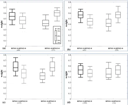
proposed combination scheme correctly identifies the neighbors in estimating the weights for each candidate model resulting in an improved skill from the WCI-based probabilistic forecasts. w ei gh t w ei gh t w ei gh t w ei gh t (a) (c) (b) (d)

RPSS1>0,RPSS2>0 RPSS1<0,RPSS2<0 RPSS1>0,RPSS2>0 RPSS1<0,RPSS2<0

RPSS1>0,RPSS2>0 RPSS1<0,RPSS2<0 RPSS1>0,RPSS2>0 RPSS1<0,RPSS2<0

(60) (37) (65) (29) (109) (19) (60) (37) (65)

(115) (19) (16)

Figure 2.6: Box-plots of weights of the disaggregated GCM forecasts and reforecasts in the proposed combination scheme for different months: (a) January; (b) April; (c) July; (d) October. Weights are grouped by pooling grid points Solid (Dotted) box-plots represent the weights for the disaggregated climate forecasts (reforecasts). Numbers in the parenthesis indicate the number of grid points that have RPSS1 >0 and RPSS2 >0 and RPSS1 < 0 and

2.5 Discussion

With regard to the first question, we identified the best model at each grid point based on RPS (Figures 2.7 and 2.8). Figure 7 shows the best model for the two forecasting periods in the selected months over the four seasons, whereas Figure 8 summarizes the total number of grids in which each model has the lowest RPS for each month. From Figures 7 and 8, WCI is the best performing model and reforecasts emerges as the next best model with disaggregated forecasts being the best in only a few grid points for the month of July. Improvements from the combined forecasts is widespread and all over the country during the summer and fall months (Figures 2.7-2.8). During winter and spring months, the improvements from the combination are found predominantly over the Sun Belt during January and April as well as over the upper Mid-West and Mid-Atlantic states in the 1stbiweek of April. From Figure 2.8, WCI-based forecasts perform better during all biweeks over the year with the exception being in 1stbiweek of February and 2ndbiweek of December when reforecasts perform better for many grid points within the continental United States. Thus, it is clear that even though the performance of disaggregated forecasts performs the best in only a few grid points, combining reforecasts and disaggregated ECHAM4.5 forecasts using the proposed combination scheme result in reduced RPS over the continental United States.

Figure 2.8: Number of grid points under which each forecasts (DF, RF and WCI) during the first fifteen days (a) and the second fifteen days (b) have the lowest RPS for each month over the continental United States.

0 20 40 60 80 100 120 140 160

Jan Feb Mar Apr May Jun Jul Aug Sep Oct Nov Dec

N u m b er o f gr id s DF RF WCI 0 20 40 60 80 100 120 140 160

Jan Feb Mar Apr May Jun Jul Aug Sep Oct Nov Dec

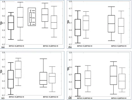
forecasts. Recently, Weigel et al., (2008) carried a theoretical study to investigate under what situations multi-model combinations can outperform individual models. It was concluded that multimodel combination results in a well-dispersed forecasts by reducing the overconfidence of the individual models. For instance, it is common for forecasts from numerical models to indicate high probability of occurrence of one particular tercile category (e.g., 90% probability of below-normal precipitation). Weigel et al. (2008) suggested methods to estimate the dispersion parameter (), which ranges from zero to one, based on the forecast ensembles. When  is zero (one), the distribution of forecasts is well-dispersed (overly dispersed). Appendix A provides details on estimating  for a given forecast. For additional details, see Weigel et al. (2008).

Figure 2.9 compares the estimated  between disaggregated GCM forecasts (solid box plots) and reforecasts (dotted box plots) with RPSS1 and RPSS2 of the WCI forecasts being above

WCI forecasts. As the length of reforecasts increases, weather-climate combination forecasts could be evaluated based on split-sample validation as well as by developing real-time experimental forecasts to understand their utility in improving medium-range weather forecasts.

Figure 2.9: Box-plots of dispersion parameter,, of the disaggregated GCM forecasts (solid box) and reforecast (dotted box) in the proposed combination scheme for different months: (a) January; (b) April; (c) July; (d) October. Dispersion parameters are grouped in such a way with RPSS1 and RPSS2 of WCI being greater than and lesser than 0.

(a)

(c)

(b)

(d)

β

β

β

β RPSS1>0,RPSS2>0 RPSS1<0,RPSS2<0

RPSS1>0,RPSS2>0 RPSS1<0,RPSS2<0 RPSS1>0,RPSS2>0 RPSS1<0,RPSS2<0

2.6 Summary and Conclusions

Chapter 3 A Framework for Incorporating Ecological Releases in

Sustainable Reservoir Operation

3.1 Introduction

Explicit consideration of ecological flow regimes is not commonly included in current reservoir operation practice (e.g., Yeh, 1985; Labadie, 2004) that specifies a minimum release, which is determined based on long-term flow conditions and anthropogenic demands. On one hand, due to the competing needs, outflow from the reservoir might not be able to sustain ecological health of the river since minimum environmental flow is usually determined based on agreement among stakeholders, especially downstream communities. On the other hand, water releases for hydropower generation are usually not in conflict with ecological requirements since tail water from turbines typically is returned to the river. Too much water released after hydropower generation would also alter the flow regime that potentially leads to ecological damage. Therefore, it is challenging to explicitly consider ecological flow amount and variation requirements in multi-purpose reservoir operation planning; they are usually considered as hard constraints to meet only a constant minimum release (Jager and Smith, 2008).

This operation mode is not practical, however, for a large reservoir that serves multiple purposes, including flood control, domestic water supply, irrigation supply, and hydropower generation. Modified operation rules are needed to meet these anthropogenic demands while minimizing the potential damage to the downstream ecological system.

Flow regime-based ecological consideration in multi-purpose reservoir operation has drawn much attention in the research community (e.g., Cardwell et al., 1996; Richter and Thomas, 2007). Cardwell et al. (1996) proposed a multi-objective optimization model for monthly reservoir operation that considers anthropogenic water demands as well as fish habitats. Jager (2008) suggested three steps to conceptually bring multi-objective reservoir operation closer to meeting the goal of ecological sustainability. Identification of features of flow variation that are essential for river health and quantification of these relationships provide a comprehensive understanding of the river ecosystem. Richter et al. (2007) provided a descriptive framework for modifying reservoir operation to restore ecological flow regime.

since historical flows are not necessarily representative of future daily flows. Also, reservoir inflow forecast information is generally not available or reliable beyond a certain time, e.g., one month or one season depending on the inflow forecast model. Recently, Yang and Cai (in press) investigated a multi-objective optimization model that minimizes flood damage and maximizes fish diversity by generating synthetic daily inflow data where the statistical characteristics of historical data was assumed to be preserved.

Restoration of downstream flow regime cannot be assessed based on a short time period; it may take a decade or even longer to know any successful restoration of the ecological environment to that of pre-impact period. Hence, an adaptive framework for reservoir operation is needed to identify daily releases based on inflows for restoring the flow regime in the long term.

The objectives of the study are to: 1) propose an adaptive reservoir operation framework for restoring the flow regime to pre-impact conditions; 2) implement and test the framework using a daily reservoir operation model to incorporate anthropogenic water needs and ecological flow releases; and 3) study the tradeoff between meeting anthropogenic water needs and ecological flow requirements.

optimization is introduced in this section. Results of application of this framework for an illustrative example are discussed in Section 3.3. The assumptions of this work and framework extension are discussed in Section 3.4, followed by concluding remarks in Section 3.5.

3.2 Methodology

3.2.1 Framework Description

A four-step framework (Figure 3.1) for multi-purpose reservoir operation to restore natural flow regime is proposed.

The collection of IHA parameters reflects the magnitude, duration and timing of hydrological variables. Five groups of hydrological variables were proposed and each group corresponds to its own ecological influence. For example, the magnitude of monthly mean flow reflects the habitat availability for aquatic organisms, soil moisture availability for plants and availability of water for terrestrial animals (Ritcher et al., 1996). To determine the relation between hydrological parameters and their possible ecological effects on a river system requires additional site-specific knowledge and cooperation from river managers and ecologists. For example, some species are usually sensitive to low flow and high flow conditions, and mean flow in specific months that may influence fish spawning. Yang et al. (2008) used a data mining approach to identify hydrological indicators related to fish community and generated a quantitative function between an ecological target index and the identified hydrological indicators for upper Illinois River.

For naturally flowing rivers, long term distribution of each hydrological flow parameter reflects the characteristics of the ecological system to which the aquatic system has been adapted. Range of Variability Approach (RVA) (Richter et al., 1998) is employed to evaluate hydrological flow alterations induced by disturbance such as reservoir operation to the natural flow conditions. The 33rdand 67thpercentile of the flow parameter distribution in the pre-impact years are used as the critical values to divide the distribution into three categories, namely, low, medium and high categories. In the pre-impact years, about the same number of years falls in each category. Let N_{i pre,} and N_{i post,} represent the number of pre-impact and

categoryi. ThenDi is the difference betweenNi pre, andNi post, . The absolute value ofDi isMi,

which represents the degree of alteration, as represented in Equation 3.1.

, ,

| | | | 1, 2,3

i i i post i pre

M  D  N N i  … (3.1)

Though Di is not directly used in RVA analysis, it usually reflects the flow impact of reservoir operation. For example, when a large portion of outflow is needed to meet anthropogenic demand in some months, there will be many years when the monthly average flow parameter falls in the low category for those months. RVA analysis is done for all three categories and for all ecological flow parameters under consideration. Summation ofMiover the three categories of all flow parameters is the total number of mis-hits; its magnitude reflects the degree of flow alteration. RVA aims to compare the distribution of each flow parameter between pre-impact and post-impact period by discretizing the distribution into three categories. Ideally, hydrological alteration over all three categories should be zero, indicating that the reservoir operation has no impact on the hydrological flow regime.

range based on past data neglects future inflow condition as well as reduces the flow variability.

Inflow

Figure 3.1: An adaptive framework of reservoir operation

To better preserve the flow regime variability, a new approach based on inflow conditions is proposed, which considers all three categories of the flow parameters in pre-impact years. By examining the forecasted inflow condition when deciding the reservoir operation in the decision horizon, the high category of the flow parameter in the pre-impact years is chosen as the target range for the parameter if the inflow is above normal. If the forecasted inflow is below normal, the low category of the flow parameter in the pre-impact years is chosen as

Identify a subset of ecological parameters, which have the most influence on the downstream ecological system

Set target range for parameters of interest conditioned on reservoir inflow

Daily reservoir operation decision support system

the target range. This approach enables conditional determination of the release instead of using a fixed target range making the reservoir operation framework adaptive.

The third step is to formulate a daily reservoir operation optimization model to determine daily releases that meet different water demands effectively. Various pieces, such as flow balance, ecological mis-hits function, water supply and hydropower generation, of this optimization model are described in Section 3.2.2. A key input to this model is the inflows that are based on streamflow forecasts. Hence, the releases are determined adaptively contingent on the forecasted inflow instead of a static release policy.

Finally, site monitoring and evaluation phase of the framework could provide information on how the river ecosystem responds to the actual ecological releases and help adjust and fine-tune the models and procedures in the framework.

following section presents a daily reservoir operation optimization model to explicitly consider ecological flow requirement and other anthropogenic water demands.

3.2.2 Mathematical Formulation of Reservoir Operation

A multi-purpose reservoir operation optimization model is developed to estimate water releases for the different anthropogenic uses, as well as ecological flow needs. The sets of constraints and necessary expressions for defining the objective function are described below.

Flow balance

Equation 3.2 describes the reservoir flow balance, where s_j is the end-storage on day j, J is

total number of days in the decision horizon, I_jis inflow to the reservoir on day j, x_j is

ecological release on day j, and R_j is the non-ecological release on day j, e_j and sp_j

represent evaporation and spillage, respectively, from the reservoir on day j. Reservoir

storage is constrained by Equation 3.2, where smin is the user-defined acceptable minimum

storage and smax is the user-defined acceptable maximum storage.

s_j s_j1  I_j R_j x_j ws_j sp_j  j {1, 2,.., }J … (3.2)

Mis-hits in ecological flows

The following set of equations is included to represent the six flow parameters considered in this study, and how they are used to calculate the number of mis-hits, i.e., frequency of falling outside of the target range for each parameter.

1 1 J j j x P J 





P₂ x_j  j {1, 2,.., }J … (3.5)

2 0 3 ₃ j t t x P  





6 0 4 7 j t t x P  





2 0 5 3 j t t x P  





6

0

6 ₇ {1, 2,.., 6} j t

t

x

P j J

 





2

{1, 2,.., }

j i

j

P x

h j J

C 

   … (3.10)

2 3 0 / 3 {1,2,.., 2} j t i t j P x

h j J

6 4

0

/ 7

{1, 2,.., 6}

j t

i t

j

P x

h j J

C       



{1, 2,.., 2}

j t

i t

j

P x

h j J

C       



{1, 2,.., 6}

j t

i t

j

P x

h j J

C       



(1 ) 1 {1,2,.., } 2,3,...,6

J

i j j

h j J i



     



(1 ₁i) arg _mini ₁i arg _maxi 1, 2,..,6

i

P  q t et  q t et  i … (3.16)

2 arg min (1 2) arg max 1, 2,.., 6

i i i i

i

P q t et  q t et  i … (3.17)

6

1 2

1

( i i)

total i

q q M



 



… (3.18)

1, ,2 {0,1} 1, 2,..,6

i i i

j

q q h   i … (3.19) i _{{0,1} 2,3,..,6 {1, 2,... }}

j

h   i  j J … (3.20)

Equation 3.4 represents the monthly mean flow, P1. xj is the release in day j, and J is the

total number of days in the month. This flow parameter is constrained by Equations 3.16 and 3.17 to fall within the specified target range (defined by 1

min

target and 1

max

target .) If the flow

parameter fell outside of the target range, then the binary variables 1 1

q and 1 2

q are used to

indicate whether P1 is greater than target1max ( 1 1

q =1) or less than 1 min

target ( 1 2

binary variables are used to count the number of mis-hits in Equation 3.18, where M_total is total number of mis-hits.

Equations 3.5, 3.10 and 3.15 are collectively used to represent the monthly 1-day minimum flow parameter, P2. The binary variable h2jis introduced to indicate when the monthly 1-day

minimum occurs and to ensure that P₂ is assigned the appropriate value. The constant

C

Similar sets of constraints are included to represent monthly 3-day minimum (P₃), monthly

7-day minimum (P₄), monthly 3-day maximum (P₅), and monthly 7-day maximum (P₆).

Corresponding variables_q1i_, 2 i

q and i j

h are introduced to ensure that variable P_i is assigned the

appropriate value based on flow valuesx_j, and all mis-hits are flagged and added in Equation

3.18.

The total count of mis-hits, M_total, is then used either as an objective function in scenarios focused on minimizing ecological flow alteration, or as a constraint (Equation 3.21) in scenarios where the flow alteration is limited by some target number (g) of deviations from pre-impact conditions.

total

M  g

Water supply

Equations 3.22 and 3.23 are included to ensure that at least fraction rof water demand is satisfied, wherews_j is the release for water supply on day j, and wd_jis the daily water

demand.

_{1 1}

J J

j j

j j

ws r wd

 

 





… (3.22)

j j

ws wd  j {1, 2,.., }J _{… (3.23)}

Hydropower generation

Hydropower generation is represented usually as a function of water released to turbines and elevation difference between turbines and water level in the reservoir. This depends on the bathymetry of the reservoir and is characterized by storage-elevation curve, which is unique for each reservoir (see an example in Figure 3.2 (a)). For large reservoirs where elevation fluctuation is not a critical factor in hydropower generation or where hydropower generation is mainly flow-dependent, an alternative approach is to assume a constant reservoir water elevation (Loucks et al., 2005), but this is not generally the case. The nonlinear relation between storage and elevation can be explicitly modeled by using a piece-wise linearization approach (D’Ambrosio et. al., 2010; Goor et al., In press).

For day j, the daily average storage, s_j, is calculated as the average of the daily initial

storages_j1 and end-of-day storage s_j , as shown in Equation 3.24. The storage axis is

associated with interval k. At the boundary break points, b_0,j is associated with the first

break point and b_{K j1,} is associated with the last break point. _{k j,} is a coefficient in the range of [0,1], and it represents a weight for day jassociated with break point k. To find an estimate

of elevation corresponding tos_j, first the pair of break points adjacent to _

j

s in the storage axis is determined; then the elevation for these break points are weighted to estimate the

elevation. The weights are determined based on the relative location of s_j compared to the

two adjacent break points. Equations 3.27-3.30 are used to find the two adjacent break points. The weights (_{k j,} ) corresponding to these two adjacent break points are used to relate

(Equations 3.25-3.26) the storage (stk) at these break points to _

j

s . Then the elevations associated with these adjacent break points are combined using the corresponding weights (Equation 3.31) to estimate the elevation e

j

h in day j. These equations are shown below.

_

1

(

) / 2

{1,2,.., }

j _{j j}

s



s



s

 

j

J

_

, 1

{1, 2,.., }

K

j _{k j k}

k

s  st j J







, 1

1 {1, 2,.., }

K k j k j J     





b



0

b



0

1 ,

( ) {1, 2,.., }

K e

j k j k

k

h  f st j J



Figure 3.2: (a) Linearization for the storage-elevation curve; (b) Two-dimensional linearization for hydropower generation.

1,j

b b_2,j b_{k j,} b_{K1 1, j}

1 2 1

1, 2,

( ) ( )

k K

j j

st

st

st

st





( ) (





)

1 ( ) f st 2 ( ) f st

( _k)

f st _ j s e j h Elevation () f Storage

1 2 2

1, 2,

( ) ( )

k K

j j

q q q q

  ( ) (k j_, K j_2,)

1,j

b b2,j bk j, bK2 1, j

Release Elevation 1 y l y _ j x 2 y 1 l y_ 1,j  2,j  , l j  ~

( , )k l f q y e

j

h ~

1

( _k , )_l

f q_ y

_ e j j

(x ,h )

f

Hydropower contour

(a)

The estimated elevation ( e j

h ) corresponding to average daily storage s_j on day j and daily

release x_ j are combined to estimate the hydropower generated on day j, expressed as

energy Ej produced on day j. The Energy-Elevation-Storage-Release relationship, which is

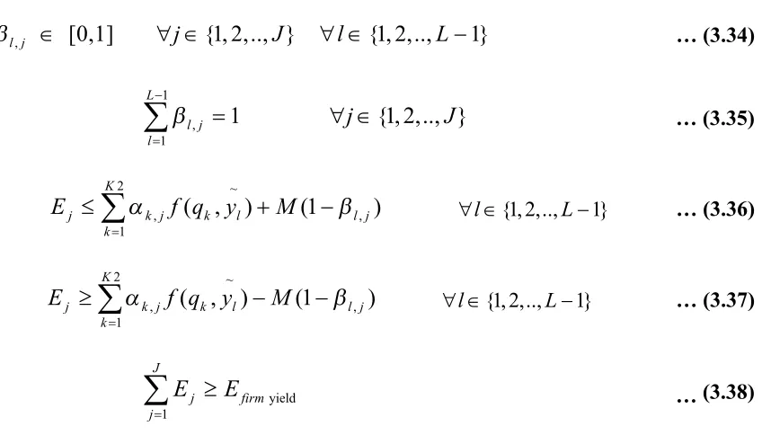
non-linear, is descretized and this non-linear function is represented, as before, using piece-wise-linear approximation. The elevation axis is discretized into Lintervals with (L+1) break points (Figure 3.2b). The variable yl represents the elevation at break point l. A set of binary

variables (l j, ; l = 1,2,.., L, j=1,2,..,J) is used to indicate the interval in the elevation axis,

and is used to determine the break point closest to e j

h on day j (Equations 3.32-3.35). The

release axis is discretized into K2 intervals with (K2+1) break points. k j, represents the

weight on day jfor break point k; the k j, weights at the two break points adjacent to _

j

x must

be such that the weighted average of the releases q_kat these adjacent break points is equal to

_ j

x . Equations 3.36 and 3.37 are used to find the energy generated (Ej) on day jas the

weighted average (using k j, weights as corresponding to _

j

x ) of energy associated with the

midpoint y~_l for the interval in which e j

h falls. These constraints are shown below.

1

, 1 1

{1, 2,.., }

L e

j l j l l

h   y_ j J

 



{1, 2,.., }

L e

j l j l l

h   y j J







,

[0,1] {1, 2,.., } {1, 2,.., 1}

l j j J l L

       … (3.34) 1 , 1

1 {1, 2,.., }

L l j l j J      



( , ) (1 )

K

j k j k l l j

k

E  f q y M 







2 ~

, ,

1

( , ) (1 )

K

j k j k l l j

k

E  f q y M 







yield 1 J j firm j E E  



Optimization models

In this study, four scenarios were investigated. In each scenario, different objective was optimized while others were subjected to target constraints. The combinations of objectives that were optimized and constrained in the four scenarios are tabulated in Table 3.1. The structure of optimization model for each scenario is presented in Figure 3.3.

Table 3.1: Objectives that are optimized and constrained in each scenario.

Ecological flow Water supply Hydropower

generation

A ● optimized ×constrained

B ● optimized

C ● optimized × constrained

D ● optimized × constrained × constrained

A: B: Maximize ₁ J j j ws 



Minimize _{1 2}

1 ( ) N i i i q q  



s.t. Flow balance Eqns. 3.2-3.3 s.t: Flow balance, Eqns. 3.2-3.3

Water supply Eqn. 3.23 Mis-hits formulation, Eqns. 3.4-3.20 Hydropower Eqns. 3.24-3.38

C: D:

Maximize 1 2

1 ( ) N i i i q q  



Minimize 1 2 1 ( ) N i i i q q  



s.t. Flow balance Eqns. 3.2-3.3 s.t:Flow balance, Eqns. 3.2-3.3

Mis-hit formulation, Eqns. 3.4-3.20 Mis-hit formulation, Eqns. 3.4-3.20 Water supply Eqns. 3.22-3.23 Water supply Eqns. 3.22-3.23

Hydropower Eqns. 3.24-3.38 E: F:

Maximize ₁ J j j E 





s.t. Flow balance Eqns. 3.2-3.3 s.t: Flow balance, Eqns. 3.2-3.3

Water supply Eqns. 3.22-3.23 Water supply Eqns. 3.22-23 Hydropower Eqns. 3.24-3.37 Hydropower Eqns. 3.24-3.38

Mis-hit, Eqns. 3.4-3.20 Allowable mis-hits,

6

1 2

1

( i i) 3

i

q q



 



Figure 3.3:Optimization models for the different scenarios investigated in this study.

Philoptt dam, which was built during 1948-1952, is located on Smith River in the Roanoke River basin (Figure 3.4). Its main purposes are flood control, recreation and hydropower generation; the powerhouse was built in 1953 with three turbines located at 813 feet above mean sea level. Hydrological alteration in the river downstream of the reservoir due to current reservoir operation was evaluated first. In addition, four scenarios were investigated to examine whether the ecological flow requirements and anthropogenic water use can be met in a more effective manner. The optimization model formulations for the four scenarios are provided in Figure 3.3.

1950 to October 1980. The optimization model was implemented using AMPL and was solved using CPLEX 12.2.

Figure 3.4: Site location of Philoppt reservoir in Virginia.

3.3.2 Result Analysis

Evaluation of current operation

distribution by categories is different in the post-impact period. For example, only in one year the flow is in the low category, and for six years it is in the high category, resulting in increased number of occurrences (14) in the medium category. The differences in this distribution are represented in terms of mis-hits that reflect the alteration resulting as a consequence of reservoir operation. Figure 3.5 (b) shows the number of mis-hits in each category for the monthly mean flow in each month. The number of mis-hits in the July-August-September (JAS) summer season is relatively higher compared to the other months. This is reflective of the current operations where more water is released in the summer months to meet increased energy demand. As this reservoir is used primarily for hydropower, this deviation in the summer months and the increased flow alterations are consistent with current operation.

Figure 3.5: Alterations in monthly mean flow under current operation: (a) shows the shift in October mean flow between pre-impact and post-impact years; (b) presents the number of mis-hits in the three categories (low, medium, and high) for mean flow in each month.

(a)(a)

Table 3.2 provides a summary of the number of mis-hits for each of the six flow parameters corresponding to the current operations. Compared to monthly average flow, the minimum and maximum flow parameters have higher number of mis-hits. The mis-hits in 1-day minimum flow in JFM season, for example, are all higher than 20, whereas the mis-hits for the monthly average flow parameter are lower than 10. The total number of mis-hits of all six parameters ranges from 50 to 90, with more mis-hits in the summer months.

Table 3. 2: Comparison of the number of mis-hits for the alterations in the six flow parameters due to current operation.

1-day

min 3-day min 7-day min 3-day max 7-day max Monthly average mis-hitsTotal

Jan 24 14 12 10 4 4 68

Feb 22 10 4 4 2 6 48

Mar 24 16 4 4 6 6 60

Apr 26 8 10 6 4 6 60

May 16 10 4 8 4 6 48

Jun 22 8 4 6 8 6 54

Jul 10 10 8 10 12 12 62

Aug 10 10 24 16 18 14 92

Sep 10 4 18 22 16 18 88

Oct 14 4 12 14 14 14 72

Nov 16 6 10 10 8 2 52

Dec 20 8 4 6 6 6 50

Scenarios A, B, C, and D