Incorporating Uncertainties in Emission Inventories Into Air Quality Modeling

(1)

ABSTRACT

ABDEL-AZIZ, AMR. Incorporating Uncertainties in Emission Inventories into Air Quality Modeling (Under the direction of Dr. H. Christopher Frey)

In modeling ambient ozone concentrations, NOx emissions estimated based on

emission inventories are used as input to air quality models. A concern regarding the quality of ozone predictions is the uncertainty inherent in emission inventories. This work aims at developing new methodologies for quantifying uncertainty in emission inventories and propagating the uncertainty through a photochemical grid air quality model.

Time series techniques were used to develop new methodologies for developing probabilistic emission inventories. These methodologies were applied to a case study for NOx

(2)

value which is 192 t/d. The second approach showed that the total daily inventory for the year 1995 had a 95% confidence interval of 548 to 778 t/d, corresponding to an uncertainty range of -15% to +22% of the average value while the 2007 case showed an uncertainty range of -8% to +15% of the average value. Comparison of the simulated results of the two approaches with observations showed that the dependent approach produced a distribution for uncertainty that more accurately represents the observed data.

(3)

(4)

(5)

BIOGRAPHY

Amr Abdel-Aziz received his Bachelor of Science degree in Civil Engineering with Honors from Ain Shams University, Cairo, Egypt, in 1994. He then joined the American University in Cairo where he worked as a teaching assistant in the construction engineering department during the period of 1994 to 1996. During the same period, he worked as a part time design engineer at CIPRO consulting and contracting. He started his graduate studies at the American University in Cairo in 1994 where he completed a diploma in environmental engineering in 1996 and a Master of Science in environmental engineering in 2000. During the period of 1997 to 1999, he worked as a consultant to the Egyptian Pollution Abatement Project which was funded by the World Bank and the Finnish International Development Agency. In 1999, he joined the technical office of the Egyptian Minister of State for

Environmental Affairs where he worked as the manager of the environmental inspection unit during the period of 1999-2000.

(6)

ACKNOWLEDGEMENTS

This research was supported by U.S. EPA Science to Achieve Results (STAR) Grant No. R826766.

I would like to express my appreciation to Dr. H. Christopher Frey for his continuous guidance and valuable technical suggestions throughout the course of this research. Without Dr. Frey’s suggestions and guidance, this work would not have been in its current form. Appreciation is also extended to Drs. E.D. Brill and Dr. H. Devine for their continuous support and encouragement. I would like to thank Dr. D. Loughlin for his time and effort with respect to the air quality model runs. Dr. Dan was very keen to finish the model runs as quickly as possible to allow for my graduation on time.

I wish to express my gratitude and thankfulness to Dr. David Dickey from the Statistics department at North Carolina State University for his support. Dr. Dickey was extremely generous in offering an enormous amount of time and valuable technical advice especially with regards to the time series part of this research.

Many thanks to my dearest friend Ahmed Eissa for his friendship which made it easy for me to overcome homesickness. I wish to thank my friend Walid Metwally for his

continuous help and friendship. Thanks are also extended to all my friends, especially Hossam El-Agroudy, Omar El-Haggan and Tamer Samir, who for their help. I would also like to acknowledge members of the research group especially Alper Unal who helped me a lot throughout my work in this research.

(7)

(8)

LIST OF TABLES

Part II

Table 1. Maximum Allowable NOx emission Rates for Coal-Fired Boilers (lb/106 BTU) ... 30 Part III

Table 1. Summary of Database ... 59 Table 2. Hourly Capacity Factor, Emission Factor, Heat Rate and Total Emissions

Variability for the Year 1995 ... 60 Table 3. Comparison of Whole Year Data Versus Ozone Season Data for Total Emissions 61

Part IV

Table 1. Parameter Estimates for the Linear Regressions of the Transformed Hourly

Emission Factor Versus Capacity Factor ... 88 Table 2. Comparison of Mean, Standard Deviation, 2.5 and 97.5 Percentiles (lb NOx / 106

BTU) for Residuals of the Transformed Emission Factor ... 88 Table 3. Ratio of 95% Prediction Interval Width for the Predicted Emission Factor of

Individual Units With Respect to that of the Combined Data Set ... 89 Table 4. Variability of Hourly NOx Emissions at the Minimum, Mean and Maximum Values of Capacity Factor for the Combined Data set... 89

Part V

Table 1. Dickey-Fuller Test, AIC Criterion, and Parameter Estimates for Capacity Factor Models for the year 1995 ... 115 Table 2. Dickey-Fuller Test, AIC Criterion, and Parameter Estimates for Emission Factor

and Heat Rate Models for the year 1995... 116 Table 3. Simulated Versus Observed Data Comparison for the Year 1995... 117 Table 4. Uncertainty in Daily and Hourly Emissions for the Year 1995 ... 118

Part VI

Table 1. Observed and Simulated Inter-Unit Correlations of Capacity Factor and Total Emissions ... 146 Table 2. Comparison of Simulated Versus Observed Mean and Standard Deviation for

Capacity Factor, Emission Factor, Heat Rate, and Total Emissions, and of Lag 1 and 2 Autocorrelations for Total Emissions ... 147 Table 3. Comparison of Uncertainty in 1995 Simulated Daily Emissions Using Dependent

(13)

Table S-1. Cross Correlation Check of Observed Capacity Factor Time Series ... 152

Table S-2. Cross Correlation Check of Observed Total Emissions Time Series... 154

Table S-3. Simulated Capacity Factor Correlation Matrix ... 156

Table S-4. Simulated Total Emissions Correlation Matrix ... 157

Part VII Table 1. Average Daily Emissions and Stack Height Ranges for Power Plants... 183

Table 2. Correlation Analysis Results for Cells (56, 57) and (42, 43)... 183

(14)

LIST OF FIGURES

Part III

Figure 1. Example of the Hourly Capacity Factor Time Series Pattern for Allen Unit 1 - 1995 .. 55

Figure 2. Empirical Cumulative Distribution Functions of Hourly Capacity Factor for Allen Unit 1 and Belews Creek Unit 1 - 1995 ... 55

Figure 3. Example of the Hourly Emission Factor Time Series Pattern for Allen Unit 1 - 1995.. 55

Figure 4. Empirical Cumulative Distribution Functions of Hourly Emission Factor for Allen Unit 1 and Belews Creek Unit 2 – 1995... 56

Figure 5. Empirical Cumulative Distribution Functions of Hourly Heat Rate for Allen Unit 1 and Lee Unit 3 - 1995... 56

Figure 6. Example of the Hourly Total Emissions Time Series Pattern for Allen Unit 1 - 1995.. 56

Figure 7. Empirical Cumulative Distribution Functions of Total Emissions for Marshall Unit 4 and Allen Unit 1 - 1995... 57

Figure 8. Diurnal Variation in Mean Emissions for Belews Creek and Marshall Plants - 1995... 57

Figure 9. Coefficient of Variation for Hours of the Day for Belews Creek and Marshall Plants - 1995... 57

Figure 10. Autocorrelation of Total Emissions for Unit 1 of Allen Power Plant – 1995 ... 58

Figure 11. Periodogram of Total Emissions for Unit 1 of Allen Power Plant - 1995 ... 58

Part IV Figure 1. Emission Factor Versus Hour of Year for Unit 1 of the Cliff Power Plant ... 82

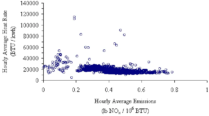
Figure 2. Emission Factor Versus Heat Rate for Unit 1 of the Cliff Power Plant... 82

Figure 3. Emission Factor Versus Gross Load for Unit 1 of the Cliff power Plant ... 83

Figure 4. Emission Factor Versus Capacity Factor for Unit 1 of the Cliff Power Plant ... 83

Figure 7. Cumulative Density Function of the Residuals Versus a Normal Distribution ... 85

Figure 8. Residuals in the Transformed Scale of the Combined Data Set for the Group (n=14497)... 85

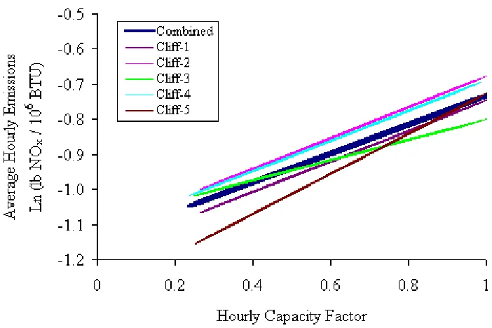
Figure 9. Combined and Specific Regressions for the 5 units in the Group... 86

Figure 10 . Cumulative Probability Plots for the Residuals of Cliff-2 Versus that of the Group... 86

(15)

Part V

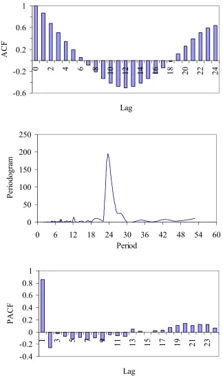
Figure 1. (a) Autocorrelation Function, (b) Periodogram, and (c) Partial Autocorrelation

Function of Unit 1 of Dan River Power Plant... 112

Figure 2. Realizations and Observed Values of Unit 1 of Dan River... 113

Figure 3. Diurnal Variation in Uncertainty for the Year 1995 ... 113

Figure 4. Uncertainty in Total Daily Emissions for the Years 1995 and 2007... 113

Figure 5. Fitted and 95% Confidence Limits of a Normal Distribution for the Year 1995... 114

Figure S-1. Percent Difference in Means of Emission Factor ... 120

Figure S-2. Percent Difference in Means of Capacity Factor... 120

Figure S-3. Percent Difference in Means of Total Emissions ... 120

Figure S-4. Percent Difference in Standard Deviations of Emission Factor ... 121

Figure S-5. Percent Difference in Standard Deviations of Capacity Factor... 121

Figure S-6. Percent Difference in Standard Deviations of Total Emissions ... 121

Part VI Figure 1. Observed Versus Simulated Correlation of Capacity Factor for the Year 1995 ... 143

Figure 2. Diurnal Variation in Uncertainty of Total Emissions from All Units (1995) ... 143

Figure 3. Uncertainty in Hourly Emissions at 12 Noon for Riverbend Power Plant for 1995 .... 143

Figure 4. Uncertainty in Daily Emissions for all Units in the Modeling Domain Using Dependent and Independent Approaches For 1995 ... 144

Figure 5. Fitted Lognormal Distribution to the Simulated 1995 Total Daily Emissions with 95% Confidence Intervals ... 144

Figure 6. Comparison of 1995 Daily Creek Power Plant Total Emissions Using Independent and Dependent Emissions Uncertainty Modeling Approaches and Observed Values. 144 Figure 7. Comparison of Uncertainty in Estimated 2007 Daily Emissions for all Units in the Modeling Domain Using Dependent and Independent Approaches... 145

Figure S-1. Percent Difference in Means of Emission Factor ... 150

Figure S-2. Percent Difference in Means of Capacity Factor... 150

Figure S-3. Percent Difference in Means of Total Emissions ... 150

Figure S-4. Percent Difference in Standard Deviations of Emission Factor ... 151

Figure S-5. Percent Difference in Standard Deviations of Capacity Factor... 151

(16)

Part VII

Figure 1. Probabilistic Power Plants NOx Emission Inventory for Day 1 of the Episode... 178

Figure 2. Realization Number 2 for Hourly Emissions of Grid Cells(55, 50) (a) and (3, 54) (b)178 Figure 3. 50 Time Series of Ozone Concentration Realizations at Cell (26, 23) for the

Independent Units Case... 178 Figure 4. 50 Time Series of Ozone Concentration Realizations at Cell (26, 23) For the

Dependent Units Case ... 179 Figure 5. Wind Speed (a) and Wind Direction from North (b) at Belews Creek Power Plant

Location... 179 Figure 6. Scatterplot of Uncertainty in Ozone at Grid Cell (56,57) versus Emissions over Four

Hours at Belews Creek Plant for 50 Uncertainty Realizations. ... 179 Figure 7. Probabilistic Maximum Hourly Ozone Levels at Cell (56, 57) (a), Cell (42, 43) (b).. 180 Figure 8. Maximum Hourly Ozone Levels at Each Grid Cell for Independent (a) and

Dependent (b) Cases... 180 Figure 9. Uncertainty Ranges of Maximum Hourly Concentration of Dependent Case (a) and

Difference in Ranges from Both Cases (b) ... 181 Figure 10. Uncertainty in Maximum Hourly Ozone Concentration for Cell (35, 33) (a), Cell

(26, 33) (b), Cell (62, 41) (c), Cell (58, 46) (d)... 181 Figure 11. Probability of Exceeding the 1-hour National Ambient Air Quality Standard for

Ozone (Dependent Case)... 182 Figure 12. Probability of Exceeding the 8-hour National Ambient Air Quality Standard for

(17)

Part I

(18)

1.0 Introduction

One of the most pervasive air pollution problems in the United States is the ozone problem. Ozone concentration exceeds the national ambient air quality standards (NAAQS) in many areas in the US and hence they are designated as non-attainment areas for ozone (EPA, 2002). Ozone health effects include breathing and respiratory problems, asthma attacks, lung damage and lower immunity disease (NRDC, 2002). Ozone is formed in the atmosphere by the photochemical reactions of nitrogen oxides (NO and NO2) and volatile

organic compounds (VOCs) which are the precursors of ozone formation. Efforts have been going on in the United States to set control strategies to decrease the emission rates of ozone precursors. The control strategy is different in different regions as it depends on the VOC/NOx ratio present in the ambient atmosphere. For high VOC/NOx ratios, termed NOx

limited regions, controlling NOx leads to the decrease in ambient ozone concentration.

Controlling VOCs in low VOC/NOx regions leads to a decrease in ozone concentration.

Power plant emissions are one of the primary sources of NOx emissions that contributes to

ozone formation in the eastern U.S.

In the process of modeling ambient ozone concentrations, NOx emissions estimated

(19)

conditions, design or fuel composition is another concern which contributes a large portion to uncertainty. Projections to future years or new meteorological scenarios also introduce uncertainties since predicting future year power loads and emissions profiles is problematic and no standard methodologies exist.

Emissions are typically estimated as the product of an emissions factors and activity data. These factors are subject to inaccuracies and uncertainties (Placet et. al, 1999). For example, an emission factor for a type of engine may be based on a very limited set of experiments. The resulting emissions factor is then applied to all similar engines in the inventory, regardless of operating conditions. Similarly, activity data can involve considerable uncertainties. Area source activity data are often based on surrogates, such as county-level population density (Placet et. al, 1999). Ideally, there is a very good correlation between activity levels and the surrogate, but this approach may introduce error. Despite the potential for introducing uncertainties using these methodologies, they are a pragmatic approach to developing inventories and represent current practice.

(20)

mechanisms and meteorological inputs must be explored, uncertainties in emission inventories contribute most to the errors in predictions of air quality models (Placet et al., 1999).

This research focuses on the development of new methodologies to quantify variability and uncertainty specifically for hourly data. Continuous Emissions Monitoring (CEM) data for NOx emissions were analyzed towards the end goal of applying these new

methodologies to develop a probabilistic emission inventory. Previous research that has been conducted to quantify variability and uncertainty in emission inventories using various statistical techniques suffered from several limitations. These limitations include the inability to account for autocorrelation in the observations of a single variable and the ignorance of dependence between different variables used in the probabilistic analysis. Often, an expert elicitation method is used to assume distributions for input parameters e.g. Hanna et al. (2001) where independence of the parameter of interest is assumed and no accounting for autocorrelation, if present, is done.

(21)

exposure parameters. He mentioned that he was uncertain whether the ignorance of these correlations biased the results or not. Winiwarter and Rypdal (2001) also used Monte Carlo simulation to assess uncertainty associated with greenhouse inventory for the year 1990 in Austria. They used expert elicitation to obtain estimates for uncertainties in emission and activity data. In the process of developing the uncertainty estimates for the total emissions for the year 1990, they did not account for dependence between emission and activity factors. Burmaster and Anderson (1994) recommended conducting correlation sensitivity analysis between input variables among 14 proposed principles of good practice of Monte Carlo simulation. Placet et al. (1999) mentioned that the dependence between variables must be specified within the model used to compute emissions using Monte Carlo simulation. Hanna et al. (1998) recommended that values of large correlations greater than 0.5 should be accounted for in the Monte Carlo resampling. Therefore, the development of new methodologies that can account for intra-unit dependence between emission and activity data and the autocorrelation present within a data set in the process of developing and preparing any probabilistic emission inventory is important.

In the process of modeling air quality in a certain geographic domain, many units of the same source category usually exist. Furthermore, these units may be owned and operated by the same company or organization. Electricity generating utilities are an example of such situation. NOx emissions from these utilities may experience some dependence especially

(22)

they might be dispatched together. Also, units within the same geographic location might experience some dependence in emissions if the generated electricity serves the same region. Therefore, accounting for the potential inter-unit dependence among correlated emissions from different units is also important in order to simulate real world conditions.

This research employed sound statistical techniques in the process of quantifying variability and uncertainty in emission inventories and in propagating this uncertainty through air quality models. The propagated uncertainty through air quality models allows for the quantification of uncertainty in the ozone predictions. This serves as a tool in the decision making process where strategies are set to control ozone precursors. Quantifying uncertainty in ozone predictions and presenting alternative control strategies to a decision maker allows for better selection of the control strategy based on uncertain information. High uncertainty in emission levels may be an obstacle for assessing cost effective reduction strategies as well as for designing emission trading programs (Winiwater and Rydpal , 2001).

1.1 Objectives

The primary objectives of this dissertation are as follows:

1. To develop novel methods for quantification of variability and uncertainty focusing on NOx emissions from coal-fired power plants.

2. To develop new methods for the creation of a probabilistic emission inventory (PEI) that account for the intra-unit dependence between different variables used in preparing the inventory.

(23)

4. To investigate the propagation of uncertainties of emission inputs through air quality models (AQM) and the possible effect on AQM predictions.

1.2 Overview of Research

The research of this dissertation focused on three main parts: development of new methodologies to quantify variability and uncertainty in hourly data, application of these new methodologies to a case study focusing on NOx emissions to develop a probabilistic

inventory, and investigation of the propagation of uncertainty of the inventory through air quality models.

This work was part of a research project titled, “Development and Demonstration of a Methodology for Characterizing and Managing Uncertainties in Emission Inventories.” The project began in October 1998. The project was supported by a grant from the National Center for Environmental Research, Office of Research and Development of the U.S. EPA under Science to Achieve Results (STAR) program and was conducted by North Carolina State University (NCSU).

The dissertation features novel methodological contributions for the quantification of variability and uncertainty in emission inventories for hourly data. Part I presents the motivations and objectives of the research. Part II presents background information and literature review on quantification of variability and uncertainty in emission inventories in addition to background on times series modeling for air pollution applications. Four manuscripts which the author plans to submit for publication in peer-reviewed journals are presented in part III and parts V through VII of this dissertation.

(24)

methodology that accounts for the dependence between variables used to develop the probabilistic inventory using regression techniques.

The manuscript presented in Part V is a methodology which employs univariate time series techniques in developing the probabilistic inventory. This methodology accounts for the autocorrelation inherent in data recorded in time and in the same time can account for intra-unit dependence between variables.

In part VI, a manuscript which provides a more generalized approach to quantify variability and uncertainty in emission inventories employing multivariate time series techniques is presented. This approach accounts for the inter-unit dependence among correlated times series in the process of developing the probabilistic inventory. In the same manuscript, the inventories developed using both time series approaches are compared. The manuscript presented in part VII investigates the propagation of uncertainty in emission inventories through a photochemical grid air quality model, where the inventories developed using both time series approaches are used and the results of each are compared. Finally, the conclusions and recommendations of this study are presented in part VIII.

(25)

1.3 References

Burmaster, D., and Anderson, P.D. (1994), “Principles of Good Practice for the Use of Monte Carlo Techniques in Human Health and Ecological Risk Assessments,” Risk Analysis, 14: 447-481.

Chao, H., Stephen, C. P. and Wan, Y.S. (1994), “Managing Uncertainties: The tropospheric Ozone Challenge,” Risk Analysis, 14(4): 465-475.

Environmental Protection Agency (EPA) (2002), “Classified Ozone Nonattainment Areas: 1- Hour Ozone Standard”. http://www.epa.gov/oar/oaqps/greenbk/onmapc.html

(accessed December 2002).

Frey, H.C. and J. Zheng (2002), “Methods for Development of Probabilistic Emission Inventories: Example Case Study for Utility NOx Emissions,” Proceedings, U.S. Environmental Protection Agency Emission Inventory Conference, Atlanta, GA.

Frey, H.C. and J. Zheng (2000), “Methods and Example Case Study for Analysis of Variability and Uncertainty in Emissions Estimation,” Prepared by North Carolina State University for Office of Air Quality Planning and Standards, U.S. Environmental Protection Agency, Research Triangle Park, NC.

Hanna, S.R., Z. Lu, Chang, J.C., Fernau, M., and Hansen, D.A. (1998), "Monte Carlo Estimates of Uncertainties in Predictions by a Photochemical Grid Model 9UAM-IV) due to Uncertainties in Input Variables," Atmospheric Environment, 32(21): 3619-3628. Hanna, S.R., Z. Lu, H.C. Frey, N. Wheeler, J. Vukovich, S. Arunachalam, M. Fernau, and Hansen, D.A. (2001), "Uncertainties in Predicted Ozone Concentrations due to Input Uncertainties for the UAM-V Photochemical Grid Model Applied to the July 1995 OTAG Domain," Atmospheric Environment, 35(5):891-903.

National Research Council (NRC) (1991), “Rethinking the Ozone Problem in Urban and Regional Air Pollution,” National Research Council, National Academy Press: Washington, D.C.

National Resources Defence Council (NRDC), Coalitoin for Environmentally Responsible Economics (CERES) and Public Service Enterprise Group (PSEG). Benchmarking Air Emissions of the 100 Largest Electric Generation Owners in the U.S. -2000; at C Page. http://www.ceres.org/reports/issue_reports.htm (accessed October 2002).

(26)

Smith, R. (1994), “Use of Monte Carlo Simulation for Human Exposure Assessment at a Superfund Site,” Risk Analysis, 14: 433-439.

(27)

Part II

(28)

This section summarizes the literature review conducted on the relevant research related to NOx emissions. First, background information on NOx emissions from coal fired

power plants is presented. Then an overview on uncertainty in emission inventories is presented. Approaches used to model air pollution problems using time series techniques are described. Finally, legislations pertaining to NOx emissions are briefly discussed.

2.0 Introduction

NOx emissions are emitted in the U.S. at a rate of about 25 million metric tons per

year. Approximately 22.5% of this amount is emitted from electric utility boilers which contribute 5 million metric tons per year (EPA, 2001). Approximately 95% of NOx emitted

from electric utility boilers is in the form of nitric oxide (NO). NO is formed as a result of two mechanisms, either fuel NOx orthermal NOx. Fuel NOx results from the combustion of

organic nitrogen in the fuel while thermal NOx is formed from the reaction between nitrogen

and oxygen in the air used for combustion. Thermal NOx, which is the mechanism

contributing most to NOx emissions from coal-fired boilers, increases exponentially with

temperature and varies with the square root of oxygen concentration (EPA, 1994). A third but less important source of NOx formation is “prompt NO”. Prompt NO is formed as a result of

the rapid reaction of atmospheric nitrogen with hydrocarbons which form NOx precursors

that are rapidly oxidized to form NO.

NOx emissions can be controlled by combustion modifications, flue gas treatment or a

combination of both. Since thermal NOx is exponentially dependent on temperature, it can be

(29)

zone or reducing air preheat temperature if preheated combustion air is used (EPA, 1994). Thermal NOx can also be reduced by reducing the amount of excess oxygen. Flue gas

treatment is accomplished through the use of selective catalytic and non-catalytic reduction. In both control techniques, ammonia is injected in a temperature window where NOx

reduction occurs by selective reaction of NH2 radicals with NO to form water and nitrogen

(EPA, 1994).

There are several types of firing technologies used for electricity generation boilers which are distinguished by firing mode. The major firing modes are cyclonic, wall fired and tangentially fired units (Cooper and Alley, 2002). NOx emission rates vary depending on the

type of fuel used and the type of firing technology. NOx emission rates which were obtained

from estimates and measurements for 18 dry-bottom wall fired boilers ranged from 0.42 to 1.77 lb/106 BTU (Castaldini, 1992 cited by Frey and Tran, 1999). The same study showed that stack testing of emissions from 19 tangentially fired boilers ranged from 0.48 to 1.64 lb/106 BTU. Also, EPA (1994) reported a range of variation for uncontrolled NOx emissions

from wall and tangentially fired pulverized coal boilers of 0.46 to 0.89 lb/106 BTU and 0.53 to 0.68 lb/106 BTU, respectively. These estimates were based on test results conducted for 200 industrial/commercial/institutional boilers. NRDC (2002) examined and compared air pollutant emissions of the largest 2000 electricity generating power plants in the U.S. These 2000 power plants account for 90% of reported industry generation emissions. The comparison of variability of NOx emission rate for coal-fired power plants for the 100 largest

(30)

2.1 Overview of Uncertainty in Emission Inventories

In this section, different views of the types of uncertainties and sources of these uncertainties in emission inventories are discussed. Previous research in quantifying variability and uncertainty in emission inventories is presented. Also, previous research pertaining to the propagation of uncertainties in inputs through air quality models is introduced.

2.1.1 Types of Uncertainties

There are several types of uncertainties in emissions inventories. Placet et al. (1999) classified three general classes of uncertainties: variability (spatial and temporal), parameter uncertainty from measurement, sampling and systematic errors and model uncertainty. They added another important source of uncertainty which is human error. According to Rowe (1993) uncertainty can be classified into four classes as follows:

• Temporal which refers to uncertainty in future states. This is the most familiar class of uncertainty as decision making under uncertainty usually deals with future states. Usually this type of uncertainty is described using a probability model which assumes that the future will behave as the past. He also added another type to the temporal uncertainty which is Temporal-Past uncertainty. Usually there is not uncertainty in the past if all events are recorded. Temporal-Past uncertainty refers to situations of failure to record past events.

• Metrical uncertainty which refers to uncertainty in measurements.

(31)

• Translational uncertainty which refers to uncertainty in communication. The results of uncertainty when presented to decision maker, stakeholder or the public might be interpreted differently. Each has a different capability and training and different perspective of understanding uncertainty. If there is no means to translate uncertainty across people from different backgrounds, misunderstanding and miscommunication of uncertainty will occur.

Rowe (1993) mentioned that all four classes are subject to variability which is a contributor to uncertainty. EIIP (1996) summarized the sources of uncertainties in emissions estimates that are obtained employing emission factors as follows:

• Variability arising from the fluctuations in the processes that produce emissions e.g. variation in fuel composition.

• Variation in ambient conditions e.g. temperature which affects the electricity production required to be produced from a power plant.

• Measurement errors in instruments.

• Models and assumptions to model complex systems

Chao et al. (1994) classified types of uncertainties that can be encountered when modeling ambient ozone as follows:

• Natural variability inherent in natural processes e.g. wind fields and meteorological conditions.

• Data uncertainty due to inaccurate measurements or insufficient data. • Model uncertainty introduced when modeling the natural processes.

(32)

Hoffman and Hammonds (1993) distinguished between two types of uncertainties in risk assessment: uncertainty due to variability which is termed type B uncertainty and uncertainty due to lack of knowledge termed type A uncertainty. When the assessment end point is a fixed quantity e.g. the risk to a specific individual, the probability distribution obtained from uncertainty analysis using Monte Carlo simulation represent a range of degrees of belief that the true quantity is enclosed in this distribution. This is termed type B uncertainty. Confidence intervals can be constructed from the distribution for which there is a given percent of chance of bounding the true value. The U.S. EPA requires that risk assessment targets the upper 95th percentile of the potentially exposed population. Therefore, the simulation of the distribution of actual exposure is required in this case. When the end point of assessment is a distribution of actual exposure, this is termed type A uncertainty. In order to distinguish between the two types of uncertainties, two dimensional Monte Carlo simulation has to be performed. This allows for estimating a confidence interval for any percentile of the obtained distribution.

The above discussion shows that most authors, except for Hofmann and Hammonds (1993), did not clearly distinguish between variability and uncertainty. Variability is the heterogeneity of data while uncertainty is the lack of knowledge of the true quantity. It is important distinguish between the two in any quantitative analysis.

2.1.2 Quantifying Variability and Uncertainty in Emission Inventories

(33)

factors are based on source testing experiments that were conducted many years ago and have poor quality ratings (Placet et al., 1999). Emission inventories are usually comprised of different source categories: natural, mobile and stationary sources. According to Placet et al. (1999), many of the methods used to estimate emissions from stationary sources introduce a worrisome degree of error in the inventory. Emissions from these sources contribute to a large fraction of the inventory and even a small percentage of error can introduce a large effect on the total inventory. Previous efforts have been conducted to quantify variability and uncertainty in emission inventories which ranged from simple to the more complex and computationally heavy statistical techniques.

Examples of simple approaches used includes Chang et al. (1996) who used fuel consumption data, actual operating schedules and AP-42 emission factors to estimate the variability in NOx emissions from point sources in the Atlanta metropolitan region. They

estimated a daily variation in emissions of 24% with respect to the emissions of a typical summer day. Van Amstel et al. (2000) developed uncertainty estimates for greenhouse emission inventories in the Netherlands based on another simplified approach. In this approach, uncertainty of each combined parameter was estimated to be equal to the square root of the sum of squares of the standard deviations of each input parameter. Lee et al. (1997) used a qualitative approach in estimating uncertainty in global NOx emissions from

(34)

emission rate for coal fired power plants per company by dividing each company’s annual emission totals by each company’s total MWhs of generation. The highest emission rate was 8.3 lb/MWh while the lowest was 2.5 lb/MWh. This revealed that fact that power plants invest differently in emissions control technology which causes inter-plant variability in emissions. El-Fadel et al. (2001) used another simplified approach to assess uncertainty in green house emissions inventory for Lebanon. They estimated the emissions using alternative experimental and theoretical factors, e.g. AP-42 factors, other than those recommended by the United Nations Intergovernmental Panel on Climate Change (IPCC). As a measure of uncertainty in the inventory, they calculated the relative deviation of CO2 emissions

estimated based on the alternative emission factors from those obtained based on the IPCC factors. They concluded a relative deviation of up to 15% which was attributed to the different carbon content of fuels in different countries and possible deviation of source behavior and control efficiencies. Expert judgment, another simplified method, has also been used to estimate uncertainty in emission inventories e.g. Gschwandtner (1993) who estimated uncertainties in VOC and NOx inventories in the U.S. for the years between 1900-1990 based

on this method.

Computationally heavy statistical techniques such as bootstrap simulation and Monte Carlo Simulation were used by some researchers to quantify variability and uncertainty in emission factors and inventories. For example, Winiwarter and Rypdal (2001) used Monte Carlo simulation to assess uncertainty associated with greenhouse inventory for the year 1990 in Austria. Frey and Tran (1999) propagated uncertainties in NOx measurement

(35)

concluded. Frey and Bammi (2002) quantified variability and uncertainty in lawn and garden engines, and for construction, farm and industrial equipment emission factors. Empirical and parametric distributions were used to quantify variability while bootstrap simulation was employed to characterize confidence intervals for the fitted distributions i.e. uncertainty. Frey and Li (2001) employed similar approaches to quantify variability and uncertainty in NOx

and total organic carbon emissions for stationary natural gas-fueled internal combustion engines. Li and Frey (2002) developed a probabilistic national per capita emission factor for volatile organic emissions from consumer/commercial use. Another example of bootstrap simulation in air quality field is the study conducted by Gatz (1995). He used bootstrap simulation to calculate the 95% confidence interval for a weighted mean of the concentrations of nine major ions in precipitation. These concentrations were sampled at ten several sites in the National Atmospheric Deposition Program.

Bootstrap technique is also a very powerful tool to treat non-traditional data sets. For example, Frey and Zhao (2002) were able to quantify variability and uncertainty in air toxics censored data sets. Also, Zheng and Frey (2001) employed bootstrap technique to quantify variability and uncertainty in mixture distributions. Other examples of probabilistic analysis of emissions include Rhodes and Frey (1997), Frey (1997), Frey (1998), and Frey et al. (1998).

(36)

was concluded that the temporal variability contributed most to the overall uncertainty. Khalil (1992) employed another statistical approach to estimate uncertainties in total global budgets for trace gases. He assumed a uniform distribution to represent emissions of methane, carbon monoxide and carbonyl sulfide from individual source categories and found an analytical solution for the probability density function of the summation of emissions from these categories. Confidence limits for the total emissions were estimated from the probability density function.

Recently, some efforts have been done to develop computer software that enables quantification of variability and uncertainty in model inputs for any probabilistic analysis. Frey and Zheng (2002) developed a prototype software tool that enables users to fit parametric distributions to data sets. The software allows for quantifying variability and uncertainty in various inputs as well as outputs of an emission inventory. They demonstrated a case study to develop a 6 month probabilistic inventory for NOx emissions for 45 coal fired

electricity generating units. Zheng and Frey (2002) introduced another software tool developed for use with the SHEDS model for quantitative risk assessment. The software tool features the use of bootstrap simulation and Monte Carlo simulation for simultaneously quantifying variability and uncertainty.

2.1.3 Continuous Emissions Monitoring (CEMs) Data

(37)

categories of sources do not represent the real temporal data for a specific time period (Placet et al., 1999). Some source categories continuously monitor their emissions. These continuously monitored data provide a rich source for information regarding variability in emissions from certain sources which if quantified can in turn provide a means to quantify uncertainties in hourly emissions for future episodes.

Emission factor are published in a report called Compilation of Air Pollutant Emission Factors, commonly called AP-42, by the U.S. EPA. A comparison for the NOx

emission factors computed using CEMs data versus those presented in AP-42 factors was done by Placet et al. (1999). They showed that the NOx emission factor derived from CEMs

data was fairly close to the factor of the AP-42 used for older boiler types that were installed before the New Source Performance Standards (NSPS) were in effect in the late 1970s. There was a huge difference between CEMs based factors and AP-42 factors for boilers subject to the NSPS or those pre-NSPS but using low NOx burners and for units using sub-bituminous

coal. This comparison showed that the emission factor was derived based on source test performed on boilers operated pre-NSPS without low NOx burners and using bituminous

coal. Placet et al. (1999) mentioned that the U.S. EPA is currently revising the emission factors in AP-42 based on CEMs data. They recommend that the U.S. EPA should give high priority to investigate uncertainty associated with emission factors derived based on CEMs data.

2.1.4 Propagation of Uncertainties in Inputs through Air Quality Models

(38)

the results of these air quality models. If emissions are not properly estimated, emissions sources may pay a larger share to decrease their pollutants than the correct one had the inventory been correct. Therefore, it is very important to quantify any uncertainty in model predictions prior to presenting to a decision maker to allow for better informed control strategies. Rowe (1999) stated that for better decision making, understanding uncertainties is a prerequisite. He recommended the use of range/confidence estimates to describe our knowledge about uncertain situations instead of using point estimates. Placet et al. (1999) pointed that errors in emission inventories can have a huge influence on ozone predictions and that estimates of uncertainties in emission inventories can help modelers explain the difference between predictions and observations. They added that the uncertainties in emissions are not well quantified and the effect of this uncertainty on air quality modeling is not fully understood. Therefore, they recommended that statistical analyses should be conducted to quantify variability and uncertainty.

(39)

using 50 simulations where simple random sampling was applied. They also found that the variability in anthropogenic volatile organic compounds (VOCs) emissions had most impact on the uncertainty in predicted ozone concentrations. Placet et al. (1999) argued that the uncertainty estimate value of 80% for VOC emitted from area sources, which was based on expert judgment, is rather high and undoubtedly contributed to the conclusion of Hanna el al. (1999) that VOCs from area sources is most contributing to uncertainty in ozone predictions. They stated that better methods should be employed to quantify uncertainty in sources of emissions that appear to contribute most to uncertainty in ozone predictions.

Hanna et al. (2001) employed the same approach used by Hanna et al. (1999) but applied to the ozone transport assessment group (OTAG) domain. They addressed uncertainties in 128 input variables including emissions, initial and boundary conditions, meteorological variables and chemistry. Elicitations from 100 experts were used to estimate uncertainties in inputs. Although they recognized the importance of including correlation among inputs, they did not account for it since there was not enough information available. The study concluded that the uncertainty in ozone concentration was most affected by the uncertainty in NO2 photolysis rate which was confirmed by comparing the correlation

(40)

A sampled Monte Carlo approach was applied by Moore and Londergan (2001) to quantify uncertainties in ozone predictions where Latin hypercube sampling was employed. They used a highly restricted sampling approach to the Monte Carlo method (MCM) in order to reduce the computational intensive aspects of applying a full MCM. They focused on quantifying the uncertainty in concentration difference between a base and a control scenario. The main objective of their study was to assess the smallest concentration difference that is significantly different from zero and to investigate the influence of uncertainties present in individual inputs on uncertainty in concentration difference between base and control scenarios. They propagated uncertainties in 168 different model inputs for emissions, chemistry, meteorology and boundary conditions. Lognormal and normal distributions were used based on expert judgment to describe the uncertainty in different input parameters investigated. In their study, they accounted for the correlation during the sampling process between: (1) temperature and VOC emissions, (2) temperature and chemical rate coefficients. Autocorrelation was accounted for in some meteorological input parameters using time series autoregressive models. They concluded that including time-dependent uncertainty had significant effects on the results and recommended the use of more realistic uncertainty models to characterize input uncertainty.

(41)

emission contributed most to uncertainties in ozone concentrations. Sistla et al. (1996) investigated the effect of uncertainty in the specification of meteorological inputs on ozone concentration patterns. They investigated the effect of using different wind fields and mixing heights representations on ozone predictions. Bergin et al. (1999) quantified the uncertainties in reactivity of volatile organic compounds, which is the term given for ozone forming potential, as a result of uncertainty in reaction rate constants.

2.2 Approaches in Modeling Air Pollution Using Time Series Techniques

In this section, an overview of some previous research which applied time series techniques to various air pollution and other environmental applications is presented.

2.2.1 Applications of Univariate time Series in Air Pollution Problems

Univariate time series has been used to model various environmental problems including air pollution. Walters et al. (1999) used univariate time series to investigate the autocorrelation structure of NOx emissions from cement kilns. They concluded that the NOx

emissions are highly autocorrelated up to lag 19 in some cases. The high levels of autocorrelation resulted in an underestimation of the standard error of mean emissions by a factor of seven to eight in some cases. They also concluded that there was high variability in NOx emissions which are attributed to changes in fuel, feed, air flow and temperatures in the

(42)

Heis et al. (2000) analyzed elemental carbon, meteorological and traffic count time series at various urban locations using spectral analysis. They were able to detect the common frequencies in the elemental carbon time series and other time series. This allowed finding the influence of traffic and long range transport on elemental carbon concentration. Sebald et al. (2000) also used spectral analysis to investigate the formation and decomposition processes of tropospheric ozone and to detect the causes of high ozone concentrations in summer. They concluded that the meteorological large and synoptic scale fluctuations affect ozone concentration at all monitoring locations in their studies. They also found a weekly periodicity for ozone concentration at one site which was caused by traffic emissions.

Sharma and Khare (2000) used univariate linear stochastic models to predict ambient maximum daily carbon monoxide concentration from vehicle emissions at a major traffic intersection in Delhi city, India. The developed models can be used for short-term, real time forecasts of maximum ambient carbon monoxide concentrations for the study region. They used monitored data for carbon monoxide ambient concentration for the period starting January 1994 to March 1997 to fit the model. This was done to satisfy the recommendation of Box et al. (1994) where they recommend keeping full history of the series so that the autocorrelation structure may be more effectively examined and hence a greater representation of the process can be achieved. Gleit (1987) used autoregressive moving average models to obtain expressions for the probability of compliance of SO2 emissions for

different averaging times.

(43)

use of time series models in quantifying uncertainty for hydrological inputs. They suggested the use of time series models to generate realizations of the underlying process that are not statistically distinguishable from the observed series. This can be accomplished using simulation techniques such as Monte Carlo simulation.

2.2.2 Multivariate Time Series Modeling

Multivariate time series models can account for the correlation among different time series. If the cause of this correlation is due to the spatial location of the stations recording the readings in time, the process may be regarded as a space-time process. Kyriakidis and Journel (1999) cited different references which concluded that geostatistaical space-time models can be expressed in terms of vector autoregressive time series models. The same paper presented an excellent review on space-time models used in geostatistical applications. These types of models are applicable for environmental applications and other fields as well. Geostatistical spaciotemporal models provide a probabilistic framework that accounts for the spatial and temporal dependence between observations. Often, in geostatiscal analyses, the focus is to develop maps for a specific phenomenon over specific time instances where the spatial aspect is more important. In other applications, the analyses may focus on the time variability of the attribute of interest where multivariate time series are usually used which are generally referred to as spatial time series (Cliff et al., 1975). Spatial time series models allows for prediction of the attribute of interest only at the specific location where the measurements were recorded. Further modeling is required in order to produce maps for the entire domain of interest (Kyriakidis and Journel, 1999).

(44)

function model which is typically decomposed into a trend component modeling some average variability of the process and a stationary residual component modeling higher frequency variability (local variability) around that trend. Kyriakidis and Journel (2000a&b) applied this view to an environmental application where they modeled sulfate deposition over Europe. They used parametric temporal trend and residual models to account for the long term and short term variability, respectively, at each monitoring location. Then, they regionalized the model parameters in space to be able to predict sulfate concentration at any unmonitored location. In the second view, the spatiotemporal process is modeled as either vectors of temporally correlated random functions in space or spatially correlated vectors of time series. The choice of the type of model in the second approach depends on which domain (space or time) is more densely informed. Without further modeling, no interpolation is possible in either class of models of the second view.

In order to model correlated point source emissions from different sources where the data is recorded in time, i.e. the time domain is the more densely informed one, a vector of time series would be the most appropriate approach. Space-time models can be expressed in terms of a vector autoregressive process (Kyriakidis and Journel, 1999). Rhouhani and Wackernagel (1990) applied the second view where they used vectors of correlated time series to model monthly piezometric data in a basin south of France. Their major concern with this approach was that predictions are limited to monitoring station locations and no prediction at intermediate locations is possible.

(45)

series models were used to model the biomass, effluent Chemical Oxygen Demand (COD) and suspended solids of a biological wastewater treatment plant.

2.3 NOx Emissions Legislation

NOx emission standards can be categorized as Federal, state and local standards. NOx

emissions reductions are determined by the most stringent among the three aforementioned standards. Federal standards include New Source Performance Standards which applies to electric utility steam generating boilers built after September 18, 1978 with a capacity greater than 73 MW. These standards limits the NOx emission rate to 0.5 lb NOx/106 BTU for units

burning subbituminous coal and 0.6 lb NOx/106 BTU for units burning bituminous and

anthracite coals (CFR, 2000). Title IV of the Clean Air Act Amendment (CAAA) addresses the control of NOx for the reduction of acid rain deposition. These requirements apply to

existing boilers and are to be achieved in two phases. Phase I, aimed at reducing NOx emissions by 400,000 tons per year between 1996 and 1999. Phase II, begins in 2000 and targets the reduction of 1.5 million tons per year. Phase I applies to dry bottom, tangentially and wall fired boilers known as group 1 while phase II applies to both groups 1 and 2. Group 2 refers to boilers not included in group 1. NOx emission limits for group 1 in phase I are 0.5

lb/106_{BTU for wall-fired boilers and 0.45 lb/10}6_{BTU for tangentially-fired boilers. Phase II}

emission limits for group 1 boilers are 0.46 lb/106 BTU for wall-fired boilers and 0.40 lb/106 BTU for tangentially-fired boilers (CFR, 2000). These limits are based upon annual averages.

NOx emissions from electric utility boilers are regulated through 2 rules by the state

(46)

(.1401) as the period beginning May 31 and ending September 30 for 2004 and beginning May 1 and ending September 30 for all other years thereafter. Emissions from Duke Power Company, which owns 8 power plants in the modeling domain of the case study of this dissertation, shall not exceed:

(a) 17,186 tons per ozone season for 2004; (b) 22,270 tons per ozone season for 2005;

(c) 16,780 tons per ozone season for 2006 and each year thereafter until revised according to Rule (.1420). Also each individual unit shall not exceed a certain NOx emission allocation which is specified in rule (.1416).

Table 1. Maximum Allowable NOx emission Rates for Coal-Fired Boilers (lb/106 BTU)

Firing Method

Fuel/Boiler Type Tangential Wall Stoke or Other

Coal (Wet Bottom) 1.0 1.0 N/A

Coal (Dry Bottom) 0.45 0.50 0.4

(47)

2.4 References

Bergin, M., Noblet, G., Petrini, K., Dhieux, J., Milford, J. and Harley, R. (1999), “Formal Uncertainty Analysis of a Lagrangian Photochemical Air Pollution Model,” Environmental Science and Technology, 33: 1116-1126.

Bergin, M., Russel, A.G. and Milford, J.B. (1998), “Effects of Chemical Mechanism Uncertainties on Reactivity Quantification of Volatile Organic Compounds Using a Three-Dimensional Air Quality Model,” Environmental Science and Technology, 33: 1116-1126.

Bortnick, S.M., and Stetzer, S. L. (2002), “Sources of Variability in Ambient Air Toxics Monitored Data,” Atmospheric Environment, 36: 1783-1791.

Box, G. E. P., Jenkins, G.M. and Reinsel, G.C. (1994). Time series analysis: forecasting and control. New Jersey: Prentice Hall.

Bras, R. and Rodriguez-Iturbe, I. (1984). Random Functions and Hydrology. Addison-Wesley Publishing Company: MA.

Chang, W., Cardelino, C. and Chang, M. (1996), "The Use of Survey Data to Investigate Ozone Sensitivity to Point Sources," Atmospheric Environment, 30(23): 4095-4099. Chao, H., Stephen, C. P. and Wan, Y.S. (1994), “Managing Uncertainties: The tropospheric Ozone Challenge,” Risk Analysis, 14(4): 465-475.

Cooper, C.D. and Alley, F.C. (2002). Air Pollution Control. Waveland Press, Inc.: IL. Cliff, A.D., Hagert, P., Ord, J.K., and Bassett, K.A. (1975). Elements of Spatial Structure: A Quantitative Approach. Cambridge University Press: New York.

Code of Federal Regulations CFR (2000). 40 CFR Part 60 and Part 75, Office of the Federal Register National Archives and Records Administration: Washington DC.

Dongen, G.V., and Geuens, L. (1998), “Multivariate Time Series Analysis for Design and Operation of a Biological Wastewater Treatment Plant,” Water Resources, 32(3): 691-700.

(48)

El-Fadel, M., Zeinati, M., Ghaddar, N. and Mezher, T. (2001), “Uncertainty in Estimating and Mitigating Industrial Related GHG Emissions,” Energy Policy, 29: 1031-1043.

Environmental Protection Agency (EPA) (2001), “National Air Quality and Emissions Trends Report, 1999,” Office of Air Quality Planning and Standards, Research Triangle Park, NC.

Environmental Protection Agency (EPA) (1994), “Alternative Control Techniques Document-NOx Emissions form Industrial/Commercial/Institutional (ICI) Boilers.” Report no. EPA-453/R-94-022, Office of Air and Radiation, Office of Air Quality Planning and Standards, Research Triangle Park, NC.

Frey, H.C. and J. Zheng (2002), “Methods for Development of Probabilistic Emission Inventories: Example Case Study for Utility NOx Emissions,” Proceedings, U.S. Environmental Protection Agency Emission Inventory Conference, Atlanta, GA.

Frey, H.C. and Y. Zhao (2002), “Quantification of Variability and Uncertainty in Air Toxic Emission Factors When Data Contains Non-Detected Values,” Proceedings, U.S. Environmental Protection Agency Emission Inventory Conference, Atlanta, GA.

Frey, H.C., and S. Bammi (2002), “Quantification of Variability and Uncertainty for Selected Nonroad Mobile Source Emission Factors,” Proceedings, U.S. Environmental Protection Agency Emission Inventory Conference, Atlanta, GA.

Frey, H.C., and S. Li (2001), "Quantification of Variability and Uncertainty in Stationary Natural Gas-fueled Internal Combustion Engine NOx and Total Organic Compounds Emission Factor," Proceedings, Annual Meeting of the Air & Waste Management Association, Pittsburg, PA.

Frey, H.C., and L.K. Tran (1999), “Quantitative Analysis of Variability and Uncertainty in Environmental Data and Models: Volume 2. Performance, Emissions, and Cost of Combustion-Based NOx Controls for Wall and Tangential Furnace Coal-Fired Power Plants.” Report No. DOE/ER/30250--Vol. 2, Prepared by North Carolina State University for the U.S. Department of Energy, Germantown, MD.

Frey, H.C. (1998), “Methods for Quantitative Analysis of Variability and Uncertainty in Hazardous Air Pollutant Emissions,” Paper No. 98-RP105B.01, Proceedings of the 91st Annual Meeting (held June 14-18 in San Diego, CA), Air and Waste Management Association, Pittsburgh, PA.

(49)

Frey, H.C. (1997), “Variability and Uncertainty in Highway Vehicle Emission Factors,” Emission Inventory: Planning for the Future (held October 28-30 in Research Triangle Park, NC), Air and Waste Management Association, Pittsburgh, PA.

Gatz, D. (1995), “The Standard Error of a weighted Mean Concentration – II Estimating Confidence Intervals,” Atmospheric Environment, 29: 1195-1200.

Gleit, A. (1987), “SO2 Emissions and Time Series Models II,” Journal of the Air Pollution Control Association, 37(12): 1445-1447.

Gschwandtner, G. (1993), “Trends and Uncertainties in Anthropogenic VOC and NOx

Emissions,” Water, Air and Soil Pollution, 67: 39-46.

Hanna, S.R., Z. Lu, Chang, J.C., Fernau, M., and Hansen, D.A. (1998), "Monte Carlo Estimates of Uncertainties in Predictions by a Photochemical Grid Model 9UAM-IV) due to Uncertainties in Input Variables," Atmospheric Environment, 32(21): 3619-3628. Hanna, S.R., Z. Lu, H.C. Frey, N. Wheeler, J. Vukovich, S. Arunachalam, M. Fernau, and Hansen, D.A. (2001), "Uncertainties in Predicted Ozone Concentrations due to Input Uncertainties for the UAM-V Photochemical Grid Model Applied to the July 1995 OTAG Domain," Atmospheric Environment, 35(5):891-903.

Heis, T., Treffeisen, R., Sebald, L. and Reimer, E. (2000), “Spectral Analysis of Air Pollutants. Part1: Elemental Carbon Time Series,” Atmospheric Environment, 34: 3495-3502.

Hoffman, F.O. and Hammonds, J.S. (1993), “Propagation of Uncertainty in Risk Assessment: The need to distinguish between Uncertainty Due to Lack of Knowledge and Uncertainty due to Variability,” Risk Analysis, 14(5): 707-712.

Khalil, M.K. (1992), “A Statistical Method for Estimating Uncertainties in the Total Global Budget of Atmospheric Trace Gases,” Journal of Environmental Science and Health, A27(3): 755-770.

Kyriakidis, P. and Journel, A. (1999), “Geostatistical Space-Time Models: A Review”; Mathematical Geology, 31(6): 651-684.

Kyriakidis, P. and Journel, A. (2000a), “Stochastic Modeling of atmospheric Pollution: A Spatial Time-Series Framework. Part II: Methodology,” Atmospheric Environment, 35: 2331-2337.

(50)

Lee, D.S., Kholer, I., Grobler, E., Rohrer, F., Sausen, R., Klenner, L., Oliver, J.G.J., Dentener, F.J. and Bouwman, A.F. (1997), “Estimation of Global NOx Emissions and Their Uncertainties,” Atmospheric Environment, 31: 1735-1749.

Li, S., and H.C. Frey (2002), “Methods and Example for Development of a Probabilistic Per-Capita Emission Factor for VOC Emissions from Consumer/Commercial Product Use,” Proceedings, Annual Meeting of the Air & Waste Management Association, Pittsburg, PA.

Moore, G., and Londergan, R. (2001), “Sampled Monte Carlo Uncertainty Analysis for Photochemical Grid Models,” Atmospheric Environment, 35: 4863-4876.

National Research Council (NRC) (1991), Rethinking the Ozone Problem in Urban and Regional Air Pollution, National Academy Press: Washington, DC.

National Resources Defence Council (NRDC), Coalitoin for Environmentally Responsible Economics (CERES) and Public Service Enterprise Group (PSEG). Benchmarking Air Emissions of the 100 Largest Electric Generation Owners in the U.S. -2000; http://www.ceres.org/reports/issue_reports.htm (accessed October 2002).

Placet, M., Mann, C.O., Gilbert, R.O. and Niefer, M.J. (1999), “Emissions of Ozone Precursors from Stationary Sources: A Critical Review,” Atmospheric Environment, 34: 2183-2204.

Rhodes, D.S., and H.C. Frey (1997), “Quantification of Variability and Uncertainty in AP-42 Emission Factors Using Bootstrap Simulation,” Emission Inventory: Planning for the Future (held October 28-30 in Research Triangle Park, NC), Air and Waste Management Association, Pittsburgh, PA.

Rhouhani, S., and Wackernagel, H. (1990), “Multivariate Geostatistical Approach to Space-Time Data Analysis,” Water Resources Research, 26(4): 585-591.

Rowe, W. (1993), “Understanding Uncertainty,” Risk Analysis, 14(5): 743-750.

Sebald, L., Treffeisen, R., Reimer, E., and Heis, T. (2000), “Spectral Analysis of Air Pollutants. Part2: Ozone Time Series,” Atmospheric Environment, 34: 3503-3509.

Sharma, P., and Khare, M. (2000), “Real-Time Prediction of Extreme Ambient Carbon Monoxide Concentrations due to Vehicular Exhaust Emissions Using Univariate Linear Stochastic Models,” Transportation Research Part D, 5: 59-69.

(51)

Van Amstel, A., Olivier, J.G.J., Russenaars, P. (Eds.) (2000), “Monitoring of Greenhouse Gases in the Netherlands: Uncertainty and Priorities for Improvement,” Proceedings of a National Workshop: Bilthoven, The Netherlands.

Walters, L.J., May, M.S., Johnson, D.E., Macmann, R.S. and Woodward, W.A. (1999), “Time-Variability of NOx Emissions from Portland Cement Kilns,” Environmental Science and Technology, 33: 700-704.

Winiwarter, W., and Rypdal, K. (2001), “Assessing the Uncertainty associated with National Greenhouse Gas Emission Inventories: A Case Study for Austira,” Atmospheric Environment, 35: 5425-5440.

Zheng, J., and H.C. Frey (2001), "Quantitative Analysis of Variability and Uncertainty in Emission Estimation: An Illustration of Methods Using Mixture Distributions," Proceedings, Annual Meeting of the Air & Waste Management Association, Pittsburg, PA.

(52)

Part III

QUANTIFICATION OF HOURLY VARIABILITY IN NO

X

EMISSIONS

FOR COAL-FIRED POWER PLANTS

(53)

Abstract.

The objectives of this paper are to: (1) quantify variability in hourly utility NOx

emission factors, activity factors, and total emissions; (2) investigate the autocorrelation structure and evaluate cyclic effects at short and long scales of the time series of total hourly emissions; (3) compare emissions for the ozone season versus the entire year to identify seasonal differences, if any; and (4) evaluate inter-annual variability. Continuous Emissions Monitoring (CEM) data were analyzed for 1995 and 1998 for 32 units from 9 baseload power plants in the Charlotte, NC airshed. Typical 95 percent ranges of hourly variability over all hours of the year exceeded ±40%. The total emissions has a strong 24 hour cycle attributable primarily to the capacity factor. Typical ranges of the coefficient of variation for emissions at a given hour of the day were from 0.2 to 0.3 during the daytime and as much as 0.45 during the night. Little difference was found when comparing weekend emissions with the entire week or when comparing the ozone season with the entire year. There were substantial differences in the mean and standard deviation of emissions when comparing 1995 and 1998 data, indicative of the effect of retrofits of control technology during the intervening time. The wide range of variability and its autocorrelation should be accounted for when developing probabilistic utility emission inventories for analysis of near-term future air quality episodes.

Implications.

Emission inventories are widely used for air quality management decisions. However, the uncertainty in these numbers is typically ignored or treated only qualitatively. This work represents an effort to develop and promote the use of quantitative techniques for characterizing both variability and uncertainty. When making estimates of uncertainty for near-term future episodes, there is substantial uncertainty in utility NOx emission on the order