Metrology Artifact Design

(1)

ABSTRACT

Folkert, Karalyn Faith. Metrology Artifact Design. (Under the direction of Thomas A. Dow)

Part acceptance is based on dimensional inspection by comparison to the tolerance specifications of the part drawing. These measurements are often taken on Coordinate Measuring Machines (CMMs); but the dynamics of the machine will influence the overall measurement. Traditionally, a calibration artifact determines the static influences of the machine such as machine geometry. The goal of this project is to design and fabricate a calibration artifact that will test a CMM both statically and dynamically and determine the effects of those influences.

(2)

(3)

METROLOGY ARTIFACT DESIGN

KARALYN F. FOLKERT

A thesis submitted to the Graduate Faculty of North Carolina State University

in partial fulfillment of the requirements for the Degree of

Master of Science

MECHANICAL ENGINEERING NORTH CAROLINA STATE UNIVERSITY

Raleigh, NC 2005

APPROVED BY:

________________________ __________________________

(4)

BIOGRAPHY

(5)

ACKNOWLEDGEMENTS

I will always be grateful for the invaluable experience and trials that come with pursuing a Masters. There have been many people who have been influential throughout these last two years at NC State. I would personally like to thank a number of them.

• Dr. Thomas Dow, my advisor, for continuing to push me to perfection. His insatiable desire for detail and knowledge has been inspirational. Thank you for taking the time to explain anything and everything that I did not understand pertaining to research.

• Ken Garrard, who spent countless hours with me and Matlab. I will always be amazed by all that you know. Thank you for your patience when I know you’ve been extremely busy with other work.

• Alex Sohn, for showing me some of the ins and outs of machining. I appreciate your expertise that you shared with me on the ASG and the milling machine.

• Dr. Jeffrey Eischen and Dr. Ron Scattergood, my committee members, for your willingness to be a part of this research. Each of your classes have also taught me a lot.

• Brett Brocato, Nathan Buescher and Anthony Wong, for helping me out in the beginning stages of this research. You guys have been great!

• My fellow graduate students at the PEC: Karl, Witoon, Simon, Dave, Tim, Yanbo, Lucas, Rob and Nadim. I’ve thoroughly enjoyed the Friday lunches and comic relief!

• Lara Masters, for answering all my miscellaneous questions and taking care of my travel reservations and purchase orders.

(6)

• Lauren, for praying for me and being the voice of encouragement every time I needed it. I will always appreciate your listening ear.

• To my parents, Al and Judi Folkert, thanks for always supporting me in all that I do. Thank you for all your love and encouragement. I could not ask for better parents. Love you both.

• Lastly, thanks be to my Lord and Savior (Isaiah 55:9)

(7)

LIST OF FIGURES

Figure 1-1. Rotary contour gage ... 2

Figure 1-2. Moving bridge CMM [1] ... 2

Figure 1-3. Fixed bridge CMM [1] ... 3

Figure 1-4. Cantilever CMM [1]... 3

Figure 1-5. Gantry CMM [1] ... 4

Figure 1-6. Column CMM [1] ... 4

Figure 1-7. Moving bridge CMM at NCSU [9]... 5

Figure 1-8. Six degrees of freedom on a CMM axis [2]... 6

Figure 1-9. Touch trigger probe [8] ... 7

Figure 1-10. Example of lobing in the X-Z plane with a 4mm diameter ball and 20mm stylus length [3]... 8

Figure 1-11. Proportional displacement probe [8]... 9

Figure 1-12. Gauge blocks... 12

Figure 1-13. Ring gauge ... 13

Figure 1-14. Ball bars [13]... 14

Figure 1-15. Hole bar... 14

Figure 1-16. GeostepTM 10 [14] ... 15

Figure 1-17. Ball plate [11]... 16

Figure 1-18. Ceramic hole plate [15]... 16

Figure 1-19. Modular space frame [16] ... 17

Figure 1-20. (a) Regular geometric shapes to simulate (b) a freeform object such as a turbine blade... 18

Figure 1-21. R-type MWS around the circumference of a cylinder ... 18

Figure 1-22. Form profile of a MWS with corresponding amplitude spectrum [18] ... 19

Figure 2-1. Ring gauge drawing and 3-D image with dimensions ... 20

Figure 22. 6 Hz sine wave (left); FFT frequency response with peak magnitude of 4 and -90° phase at 6 Hz (right) ... 24

Figure 2-3. Addition of multiple sine waves (left); FFT frequency spectrum (right)... 25

Figure 2-4. Concatenation of two single frequency sine waves (left); FFT frequency spectrum (right)... 25

Figure 2-5. Eight single frequency sine waves placed side by side (left); FFT frequency spectrum (right)... 27

Figure 2-6. Swept sine wave on the OD/ID of the ring ... 28

Figure 2-7. FFT of the first quadrant of the swept sine wave (5µm amplitude) on the ID.... 30

Figure 2-8. FFT of swept sine wave with maximum amplitude of 5µm and 20,000 points.. 31

Figure 2-9. Theoretical second-order dynamic system... 32

(11)

Figure 3-2. Setup for machining of the ring gauge with the FTS on the ID... 37

Figure 3-3. First mode shape of natural frequency ... 38

Figure 3-4. Open loop characteristics of the FTS ... 40

Figure 3-5. Simulink model of FTS control... 42

Figure 3-6. Cubic fit of PZT displacement ... 42

Figure 3-7. Schematic of Al ring cross section... 43

Figure 3-8. Setup with FTS and ring gauge... 44

Figure 3-9. Calibration data of LVDT with best-fit line... 45

Figure 3-10. LVDT measurement of entire swept sine wave ... 46

Figure 3-11. Surface profile of ring gauge with bolts in place ... 47

Figure 3-12. Cross section of ring attachment to spacers ... 47

Figure 3-13. Surface profile of ring gauge with bolts removed... 48

Figure 3-14. Ring gauge in a horizontal orientation on CMM (left) and scanning probe in contact with ring (right) ... 49

Figure 3-15. Measurement of the swept sine wave on the ID (left) and measurement of the roundness of the gauge (right) ... 49

Figure 3-16. Experimental setup to machine swept sine wave on OD of cylinder and the air-bearing LVDT used to measure the final shape... 51

Figure 3-17. Cap gage reading of 2.5µm amplitude input (left); LVDT measurement of sine waves (right) ... 51

Figure 3-18. Swept sine wave output thru the HV amplifier as seen on an oscilloscope... 52

Figure 3-19. Chip formation during machining with associated angles [23] ... 53

Figure 3-20. Probe compensation concept [20] ... 54

Figure 3-21. Top subplot is the expected measurement and bottom is actual LVDT measurement ... 55

Figure 3-22. Setup of LVDT calibration (left), and determination of calibration slope (right) ... 56

Figure 3-23. Profilometer measurement of swept sine wave... 57

Figure 3-24. System characteristics of the FTS with larger view of phase from 1-600Hz.... 58

Figure 3-25. Hysteresis loops for different amplitudes of motion for the PZTs in the FTS.. 59

Figure 3-26. Various parameters for the PI gains of the closed loop controller... 60

Figure 3-27. Comparison of closed and open loop system identifications up to 600Hz ... 61

Figure 3-28. Closed loop FTS transfer function up to 800Hz ... 62

Figure 3-29. FTS transfer function complex values and their conjugate... 63

Figure 3-30. Frequency range of transfer function increased ... 64

Figure 3-31. Expanded section of adjusted input (dots) to demonstrate altered amplitude; time relates to spindle speed ... 65

Figure 3-32. Expanded section of adjusted input (dots) to show phase-lead and amplitude reduction of input signal ... 65

(12)

Figure 3-34. New design of the ring gauge artifact ... 67

Figure 3-35. Drawing with tolerance specifications of ring gauge... 68

Figure 3-36. Ring 1 after plating with Ni build-up at two counter bores ... 70

Figure 3-37. Adjustable reamer (left); valve seat cutter (right) ... 71

Figure 3-38. Verification of plating thickness for Ring 1... 72

Figure 3-39. Profilometer measurement of a chamfer on Ring 1 ... 72

Figure 3-40. z-axis touch-off on the surface of the spacers... 74

Figure 3-41. Setup to machine each ring face flat ... 75

Figure 3-42. Profilometer measurements of first machined face of Ring 1 before (top) and after (bottom) interrupted cut... 77

Figure 3-43. Profilometer measurements of second machined face of Ring 1 before (top) and after (bottom) interrupted cut... 78

Figure 3-44. Lever-type electronic gage capture of ring centering ... 79

Figure 3-45. Lever-type electronic gage measuring tilt of the FTS... 80

Figure 3-46. Measurement of tool height ... 80

Figure 3-47. Measurement of the squareness of the tool to the ID... 81

Figure 3-48. Cross section view of probe measurement of wave; left demonstrates shanking problem with stylus... 83

Figure 3-49. Cap gage captures of the swept sine wave cut on the ID of Ring 1... 84

Figure 3-50. Cap gage captures of the swept sine wave cut on the OD of Ring 1 ... 85

Figure 3-51. Comparison of expected and actual fiducial machined on the surface ... 86

Figure 3-52. Definition of counter bore positions on the ring ... 87

Figure 3-53. Surface map of the ring near CB1 with chips at edge... 87

Figure 3-54. Surface map of the ring near one of the through holes (Side 1) ... 88

Figure 3-55. Surface map of CB5 on Side 2 opposite through hole on Side 1... 89

Figure 3-56. Surface map of through hole associated with CB2 ... 89

Figure 3-57. Surface map of counter bore 2 with ring attached to spacers ... 90

Figure 3-58. Surface map of CB2 with ring taken off mount... 91

Figure 3-59. Surface map of CB5 on Side 2... 92

Figure 3-60. Surface map of CB6 on left and zoomed in on right... 93

Figure 3-61. OD of the ring on Side 2 as measured by the NewView ... 93

Figure 3-62. ID of the ring on Side 1 as measured by the NewView ... 94

Figure 3-63. Surface finish near through hole of CB5 on Side 1 ... 94

Figure 3-64. Profilometer measurement of surface finish on the ID of Ring 1 ... 95

Figure 3-65. Profilometer measurement of surface finish on the OD of Ring 1 ... 96

Figure 3-66. Set up for the LVDT measurement of the wave ... 97

Figure 3-67. Calibration of LVDT with determined conversion factor... 98

Figure 3-68. Incremental swept sine wave measurement with the LVDT ... 99

(13)

Figure 3-71. Comparison of flat section of OD before and after fit was applied ... 101

Figure 3-72. Verification of wave with averaged data ... 102

Figure 3-73. All 12 measurements of the wave on the OD of Ring 1 ... 102

Figure 3-74. Average of measurements along with wave deviation on the OD of Ring 1.. 103

Figure 3-75. Roundness of the ring on the ID of Ring 1 ... 105

Figure 3-76. Concentricity between the flat and wave sections on the ID ... 105

Figure 3-77. Comparison of flat section of ID before and after fit was applied... 106

Figure 3-78. All 12 measurements of the wave on the ID of Ring 1... 107

Figure 3-79. Average of measurements along with wave deviation on the ID of Ring 1 ... 107

Figure 3-80. Comparison of the desired wave to the actual wave on the OD of Ring 1 ... 109

Figure 3-81. The measured wave subtracted from the compensated wave (bottom) with an expanded view at the highest frequency on the OD (top) of Ring 1... 110

Figure 3-82. Comparison of the desired wave to the actual wave on the ID of Ring 1... 111

Figure 3-83. The measured wave subtracted from the compensated wave (bottom) with an expanded view at the highest frequency on the ID (top) of Ring 1 ... 112

Figure 3-84. LVDT measurement of fiducial on the OD of Ring 1 ... 112

Figure 3-85. Illustration of ridge measurement ... 113

Figure 3-86. Determination of ridge height on the OD of Ring 1 ... 114

Figure 3-87. Determination of ridge height on the ID of Ring 1... 114

Figure 3-88. Profilometer measurement of surface finish on the ID of Ring 2 ... 115

Figure 3-89. Profilometer measurement of surface finish on the OD of Ring 2 ... 116

Figure 3-90. Roundness and concentricity of ID of Ring 2... 117

Figure 3-91. Roundness and concentricity of OD of Ring 2 ... 118

Figure 3-93. Comparison of roundness of both rings ... 118

Figure 3-94. Average of measurements along with wave deviation on the ID of Ring 2 ... 119

Figure 3-95. Comparison of the desired wave to the actual wave on the ID (Ring 2) ... 121

Figure 3-96. The measured wave subtracted from the compensated wave with an expanded view at the highest frequency on the ID on Ring 2... 122

Figure 3-97. Average of measurements along with wave deviation on the OD of Ring 2.. 123

Figure 3-98. Comparison of the desired wave to the actual wave on the OD (Ring 2)... 124

Figure 3-99. The measured wave subtracted from the compensated wave with an expanded view at the highest frequency on the OD on Ring 2 ... 125

Figure 4-1. Transfer function of the LVDT on ID of Ring 2 at (a) 1RPM, (b) 2RPM, (c) 3RPM ... 132

Figure 4-2. Transfer function of the LVDT on OD of Ring 2 at (a) 1RPM, (b) 2RPM, (c) 3RPM ... 133

Figure 4-3. Measurement of the swept sine wave on Ring 2 with different speeds on the (a) OD and (b) ID ... 134

Figure 4-4. Setup to determine dynamics of LVDT ... 135

(14)

Figure 7-1. Side mounting of rotary encoder [25] ... 147

Figure 7-2. Schematic and specifications of rotary encoder [26] ... 147

Figure 7-3. TTL incremental signals [27]... 148

Figure 7-4. 15-pin, female Sub-D connectors located on the front of the controller panel [28]... 148

Figure 7-5. Construction of a capacitance gage probe [30] ... 151

Figure 7-6. Cap gage probe with dimensions ... 153

Figure 7-7. Cap gage calibration certificate... 153

Figure 7-8. The fast tool servo without the tool shown ... 154

Figure 7-9. Cross section of the FTS with specifications ... 155

Figure 7-10. Coil assembly of a LVDT [29]... 156

Figure 7-11. LVDT output based on the position of the core [29] ... 157

Figure 7-12. Dual scale torque wrench from CDI ... 159

Figure 7-13. Dial torque wrench calibration certificate... 159

Figure 7-14. Instructions on use from CDI Operation Manual... 160

Figure 7-15. Pinout of the SCB-68 connector block... 162

Figure 7-16. “System_ID_v2.vi” front panel... 163

Figure 7-17. Simulink model of the closed loop controller with the LabView input... 164

Figure 7-18. Sample of data saved by LabView... 164

Figure 7-19. x-axis is commanded speed while y-axis is the actual speed... 165

Figure 7-20. Motor open loop step response ... 167

Figure 7-21. Verification of modeled system ... 168

Figure 7-22. Step response of both systems ... 169

(15)

LIST OF TABLES

Table 3-1. Determination of feed rate... 36

Table 3-2. Determination of minimum and maximum frequency during fabrication ... 39

Table 3-3. Individual chamfer depth measurements for Ring 1 (all values in inches) ... 73

Table 3-4. Summary of interferometer surface measurements of Side 1 ... 88

Table 3-5. Summary of interferometer surface measurements of Side 2 ... 89

Table 3-6. Side 1 surface measurements with ring attached to disk and spacers ... 90

Table 3-7. Side 1 surface measurements with ring taken off mount ... 91

Table 3-8. Side 2 surface measurements with ring taken off mount ... 92

Table 3-9. Zoomed in sections on Side 2; 2 counter bores, 2 small holes... 93

Table 3-10. Summary of statistics for all OD measurements (units µm) based on the individual errors from the average measurement value... 104

Table 3-11. Summary of statistics for all ID measurements (units µm)... 108

Table 3-12. Summary of statistics for all ID measurements on Ring 2 (units µm) ... 120

(16)

1 INTRODUCTION

The Y-12 National Security Complex (Y-12) manufactures precision workpieces for the government and private companies. Part acceptance is based on dimensional inspection by comparison to the tolerance specifications of the part drawing. In the past, Y-12 used specialized gages such as a rotary contour gage to measure a round part. Coordinate Measuring Machines (CMMs) are preferred because of their flexibility; yet this flexibility may make estimating uncertainty more difficult with additional input parameters defining the measurand. The goal of this project is to design and fabricate an artifact that can accurately predict the measurement uncertainty for a task, such as scanning around a workpiece, by determining a transfer function between the measurement and the artifact.

1.1 H

ARDWARE

Two of the dominant dimensional inspection machines are rotary contour gages and CMMs. The rotary contour gage has fewer degrees of freedom than the CMM making it less flexible. A description of each machine follows.

1.1.1 Rotary Contour Gage

(17)

while moving the probe to make a longitudinal measurement. Some machines may have dual opposing probes that are able to measure the ID, OD and thickness at the same time.

Figure 1-1. Rotary contour gage

1.1.2 Coordinate Measuring Machines (CMMs)

A CMM typically consists of three carriages that are mutually orthogonal. Each machine can have a different configuration. The most common configurations include moving bridge, fixed bridge, cantilever, horizontal arm, gantry, and column [1]. Figure 1-2 is an example of a moving bridge CMM where the three axes are able to move while the table remains fixed. The moving bridge is one of the more typical designs [1].

Figure 1-2. Moving bridge CMM [1]

(18)

moving bridge design. However, the weight of the granite table may create bending of the table [1].

Figure 1-3. Fixed bridge CMM [1]

The cantilever type CMM (Figure 1-4) uses a cantilever beam that moves left to right across the table. The z-axis is mounted on a carriage that moves in and out on the cantilever beam as the cantilever moves left to right over the table [1].

Figure 1-4. Cantilever CMM [1]

(19)

The gantry CMM (Figure 1-5) is useful for large parts because of the two, large fixed beams that the coordinate axes rest on. One carriage moves back and forth on the beams while another axis, attached to the first carriage, moves from side to side. The ram moves up and down the same as the previously described CMMs with the exception of the horizontal arm CMM [1].

Figure 1-5. Gantry CMM [1]

The column CMM (Figure 1-6) consists of a table that moves in X and Y and a fixed column. The ram is attached to the column and moves vertically. A camera is another component that can be incorporated into this design [1].

Figure 1-6. Column CMM [1]

(20)

configurations exhibit inherent geometry error that must be accounted for during static calibration. The configuration will also affect the dynamics of the machine so it is important that the designed artifact can be used on any CMM.

Displacement transducers are used to find the displacement (coordinate) of each axis of the CMM. The displacement transducers may be Moiré scales, interferometric gratings, or laser interferometers. Moiré scales, the most common, consist of fringe patterns that are made up of sine and cosine waves that are of equal amplitude but are out of phase [1]. The placement of the transducers allows a spatial reference point on the probe to be used to determine the displacement along a coordinate path in the working volume of the CMM.

Probe X

Z

Y X ProbeProbeProbe

Z

(21)

On each axis of the CMM, there are six degrees of freedom. These can be segregated into three translational components (linear positioning and mutually orthogonal straightness) and three rotational components (roll, pitch, and yaw). Furthermore, the axis pairs (XY, YZ, XZ) form three out-of-squareness elements. Three axes with six degrees of freedom plus three out-of-squareness components equal 21 geometric (parametric, volumetric) errors associated with the CMM [2]. Figure 1-8 demonstrates the six degrees of freedom on an axis.

Figure 1-8. Six degrees of freedom on a CMM axis [2]

1.1.3 Probes

(22)

1.1.3.1 Touch Trigger Probes

A touch-trigger is one type of a point to point probe. It examines the surface of a part by contacting a point on the surface, where it takes a reading, and then moves out to engage another point to inspect on the workpiece. The axes on the CMM can be moved manually or programmed to touch the surface in a pre-determined pattern. For the probe in Figure 1-9, the armature of the probe consists of three arms that rest on three sets of two balls or cylinders located 120° apart [3]. The stylus of the probe deflects when it comes into contact with the workpiece and causes one or two of the arms to lift out of its neutral position. The electronic interface notices the change and triggers the CMM to take a reading [3]. After a number of readings, the CMM can compare the measurement data to basic geometric shapes [4].

Figure 1-9. Touch trigger probe [8]

(23)

dependent on the reference plane (X-Y, Y-Z, X-Z) and the orientation and length of the stylus. Lobing will produce a variation in the out-of-roundness measurement along with repeatability errors [3].

Figure 1-10. Example of lobing in the X-Z plane with a 4mm diameter ball and 20mm stylus length [3]

1.1.3.2 Scanning Probes

(24)

Figure 1-11. Proportional displacement probe [8]

There are two methods for using the scanning probe to obtain measurements. The probe can provide feedback to the CMM to maintain a constant force on the workpiece, which requires no prior knowledge of the shape of the surface. If the shape was known, the probe could operate independently as the CMM re-traces the fabrication tool path and make a faster measurement because the path is pre-defined [6]. The accuracy of the measurement depends on the linearity and the dynamics of the probe as it responds to changes in the surface [4]. The increased number of measurement readings using a scanning probe as compared to the point to point method also improves the quality of the measurement with respect to repeatability and uncertainty.

1.2 E

XISTING

T

ECHNIQUES TO

R

EDUCE

M

EASUREMENT

E

RRORS

1.2.1 Error Map

(25)

Typically, errors are defined statically due the geometry of the CMM. The working volume is divided into regions and the position errors in each region are defined in the x, y and z directions. This error information can be put into look-up tables on the machine controller and the actual part dimensions can be determined based on compensating the machine measurements for the errors in position from the error map. The uncertainty, discussed in further detail in Section 4.1, in the measurement result will be comprised of the uncertainty of the correction factor applied to the measurement and the repeatability of that error for a specific machine position. Error mapping the entire working volume of the CMM provides one solution for calibration by correcting the slide position based on the position of the probe [9].

(26)

another carriage [10]. One way to estimate dynamic errors is to use additional sensors attached to each carriage of the CMM and to construct a kinematic model to estimate probe position [10]. However, this method only demonstrates improved measurement accuracy with single axis motion. Instead of modeling the dynamic errors of the machine, an artifact may be designed to determine the actual dynamic characteristics of the machine.

1.2.2 Calibrated Artifacts

(27)

Throughout the years, there have been a number of artifacts [2,11-17] developed to evaluate the performance of a coordinate measuring machine and/or to assist in its calibration. The artifacts may be used for a specific application or for a more generalized purpose. Artifacts may also be classified by the methods in which they are used to assess the accuracy of a CMM. Those methods include kinematic reference standard technique, parametric calibration technique, and transfer standard technique [16].

1.2.2.1 Gauge Block

One of the most straightforward methods to test CMMs is by use of a gauge block. A gauge block is a piece of metal of calibrated length. It is measured in various orientations and positions on the working volume of the CMM. A variety of gauge blocks can be used as length transfer standards [12]. The length measurement of a gauge block can be directly related to the length measurement of a part.

Figure 1-12. Gauge blocks 1.2.2.2 Ring Gauge

(28)

probed or scanned. The probed data is compared with the calibration data of the ring gauge. The lobing error is based on the geometry data comparison, and machine geometric errors, such as scale and orthogonality errors, are determined from the error pattern of circular error of the gauge [12]. The measurement of a ring gauge is appropriate for the day to day survey of CMM performance.

Figure 1-13. Ring gauge 1.2.2.3 Ball Bar

(29)

development of an error map for the CMM; the volumetric machine errors are determined using this technique without finding the probe errors [12].

Figure 1-14. Ball bars [13] 1.2.2.4 Hole Bar

The hole bar is approximately 540mm in length with an I-beam cross section. As seen in Figure 1-15, the bar includes 11 holes along the length. These holes have a diameter of 13mm with a uniform distance between any two hole centers of 50 mm. The artifact can be used to determine the 21 parametric errors of the CMM. The artifact is oriented and mounted in 17 different positions to evaluate the performance. The positions cover all the parametric errors of a moving bridge CMM. The 17 sets of measurement data are compared with the calibrated artifact database to calculate the errors. The location of the hole centers are used in the transfer method in the validation of the CMM [2].

(30)

A variation in the basic hole bar involves mounting spheres in the center of each hole to transform the hole bar from a two-dimensional artifact to one that is three-dimensional. The GeostepTM_{10, Figure 1-16, has a length of 850mm, a width of 101.6mm, and a}

thickness of 38.1mm. The ten, 19mm diameter spheres are mounted along the centerline of the beam. Center to center distance between the spheres is approximately 85mm. The center to center dimensions are varied to separate the systematic errors from the step standard. The three-dimensionality of the spheres negates the possibility of alignment or cosine errors of the artifact or positioning on the CMM because the origin of a sphere is characterized by its radius as an infinitesimal value in three-dimensional space [14]. The spheres are treated as single points rather than 3D objects.

Figure 1-16. GeostepTM_{10 [14]} 1.2.2.5 Ball Plate and Hole Plate

(31)

forces, the center dimension is susceptible to change [15]. The ball plate is predominantly used for day-to-day verification of the CMM parametric errors.

Figure 1-17. Ball plate [11]

The hole plate is very similar to the ball plate. Instead of balls configured in space, precision-machined holes are configured on the plate at qualified distances. Each hole has three points probed to determine the center. Bending of the plate does not have much effect on the center dimensions because bending would occur along the same plane as the centers. The hole plate is used for the parametric error calibration of the CMM [15].

Figure 1-18. Ceramic hole plate [15] 1.2.2.6 Space Frame

(32)

CMM [16]. The main function of the space frame is to indicate error tendencies of the machine and where adjustments are needed without representing a large amount of detail of machine errors as a whole [12]. The space frame is moved in a well-defined sequence within the working volume of the CMM. Each individual measurement is compared to the frame calibration data. By using the differences of the means and standard deviations as statistical parameters, the location of specific errors may be determined [12].

Figure 1-19. Modular space frame [16] 1.2.2.7 Modular Freeform Gauge

(33)

objects that have varying shapes because the shape must be able to be approximated by calibrated artifacts. This artifact is also not useful for concave surfaces [17].

(a) (b)

Figure 1-20. (a) Regular geometric shapes to simulate (b) a freeform object such as a turbine blade

1.2.2.8 Multi-Wave Standard

The Multi-Wave Standard (MWS) consists of several sinusoidal frequencies added together. The R-type (or roundness) form of the MWS places the waveform around the circumference of a cylinder, either on the outside or the inside. If the R-type MWS is machined on the inside, it can be used as an inner surface calibration standard. The other form is the S-type (or straightness) MWS. In this case, the waveform is machined along straight lines of the cylinder. This waveform may also be machined onto a flat surface and be used for calibration with roughness measurement instruments [18]. Figure 1-21 demonstrates a R-type MWS on the outer surface of a cylinder.

(34)

A Fourier analysis of the waveform produces an amplitude spectrum with lines at each single frequency of the wave; no other signal is present within the amplitude spectrum. This makes it insensitive to small local variations or damages. Errors in the machine will be represented by random peaks outside of the intended wave frequencies. Measurements of a MWS may give three indications about the performance of the measuring instrument. These include the overall sensitivity calibration, the spectral distortion of the profile, and the influence of filtering [18]. Figure 1-22 displays the form profile with its corresponding amplitude spectrum.

Figure 1-22. Form profile of a MWS with corresponding amplitude spectrum [18]

1.3 D

ESIGN

O

BJECTIVES

There are a number of objectives in the design of an artifact. They are as follows:

1) The artifact should be a standard shape (or several standard shapes) that can be measured on multiple machines to determine a transfer function between the artifact and the measurement.

(35)

2 ARTIFACT DEVELOPMENT

After considering the artifact standards discussed in Section 1.2.2, a ring gauge was chosen for further development. The overall attributes of the ring gauge (outside diameter (OD), inside diameter (ID), and wall thickness) can be used to exercise multiple axes of a CMM. In addition, small features can be added to the ID and OD to assess the capability of the machine to deal with small temporal and spatial variations in surface features. The ring gauge can also be measured in different orientations and positions on the CMM to cover the entire working volume.

2.1 R

ING

G

AUGE

S

HAPE

The ring’s OD will measure 8” (203.2mm) with an ID of 6” (152.4mm) and an overall thickness of 1” (25.4mm). The dimensions are the approximate size of typical parts manufactured by the sponsor. The OD will have a groove that acts as a reference surface with the features being placed onto the ID. A small through hole has been designed into the ring that will provide a reference for angular position during a measurement. Figure 2-1 illustrates the dimensions and features of the ring.

Reference surface

Feature surface

Counter bores on both

sides Reference surface Feature surface Reference surface Feature surface Counter bores on both

sides

(36)

2.1.1 Material

The material chosen for the trial fabrication of the ring gauge was Aluminum 6061-T6 because it is easy to machine. One of the attributes of Al 6061 is its high coefficient of thermal expansion (23.6µm/m-°C or 13.1µin/in-°F). The size of the part may change a significant amount depending on the temperature of its environment. For calibration purposes, it is important that the artifact not fluctuate in size. Thus, the material for the final artifact is 17-4PH stainless steel which was heat treated for maximum dimensional stability. Its coefficient of thermal expansion is 10.8µm/m-°C or 6µin/in-°F or roughly half that of the aluminum. Stainless steel cannot be machined with a diamond tool due to the amount of damage possible to the tool. For this reason, the ring is plated with electroless nickel which exhibits a non-ferrous characteristic, making diamond tool machining possible. The plating also adds to the microhardness of the stainless steel (44 Rockwell C, 430 Vickers); the actual quantity (500-700 Vickers) is dependant on the phosphorus content of the plating.

2.2 R

ING

G

AUGE

S

URFACE

F

EATURES

The small features on the surface should create a range of frequencies for evaluation of the CMM performance in the dynamic environment. There are a number of possibilities for types of features. Some of those include:

• A single frequency sine wave around the entire ring

• Addition of multiple single frequency sine waves

• Concatenation of single frequency sine waves

(37)

2.3 D

YNAMIC

A

NALYSIS

T

HEORY

The candidate surface features listed in the last section can be used to study the dynamic performance of the CMM. Each type of wave has features in the shape of a wave or combination of waves. If a measurement of a feature is made as a function of time, the apparent shape can be determined. However, it is difficult to quantify the amount of error when compared to the true wave shape. Possible sources of error may be from a shift in the actual location of the wave with the correct magnitude or the measured magnitude may be incorrect. Either scenario will add to the overall error of the CMM, but the correction factors for each error may be different. Thus, it is important to separate the major source of error: magnitude or phase. A possible solution is to convert the time domain measurement to the frequency domain.

(38)

2.3.1 Discrete Fourier Transform (DFT)

If a system is defined as f(t) in the time domain and δt is the sampled time with N samples, the DFT converts the time samples to N frequency samples. It creates a complex number with the real value as a cosine component and the imaginary value as a sine component [19]. Equation 1 represents the DFT operation.

      ₋       × =

∑

− = N kt i N kt t f k F N t π π 2 sin 2 cos ) ( ) ( 1 0 (1)

where: k = 1..N

The maximum frequency sampled is equivalent to the reciprocal of the sampling time, δt,

while the minimum frequency sampled is the reciprocal of the total time of the sample. The frequency resolution is the maximum frequency divided by the number of samples. The DFT is typically calculated using an FFT algorithm to speed up the calculation because the FFT eliminates the redundant calculations present in the DFT [19]. The results of the calculation are used to create a frequency spectrum with magnitude and phase components.

2.3.2 Single Frequency Sine Wave

(39)

Figure 2-2. 6 Hz sine wave (left); FFT frequency response with peak magnitude of 4 and -90° phase at 6 Hz (right)

If any phase was added to the sine wave in Figure 2-2, the additional phase would be apparent on the phase plot. A phase shift of 45° to the right (delaying the sine wave in time from the reference cosine wave) increases the phase value to -135°.

A single wavelength sine wave measured with multiple speeds would create the range of frequencies necessary to determine the dynamic characteristics of the CMM. However, a considerable number of measurements would be required to produce a valid transfer function.

2.3.3 Multiple Single Frequency Sine Waves

(40)

Figure 2-3. Addition of multiple sine waves (left); FFT frequency spectrum (right) The addition of multiple single frequency sine waves is the concept behind the multi-wave standard in Section 1.2.2.8. Multiple multi-waves increase the amount of frequencies for evaluation but it still requires a number of measurements to calculate a conclusive transfer function. The time domain signal is also difficult to interpret in terms of shape.

2.3.4 Concatenation of Waves

The placement of single frequency sine waves next to each other (concatenation) creates a different outcome than the addition of multiple single frequency sine waves. If a 4Hz sine wave is concatenated with a 5Hz sine wave, the frequency spectrum, in Figure 2-4, shows a decrease in amplitude and an increase in phase.

4 Hz 5 Hz

(41)

The original amplitude of both waves in Figure 2-4 was 4. However, after the FFT calculation, the peak magnitude of the sum is equal to approximately 2.5 at 4.5Hz. The concatenation of waves creates a time delay in each individual wave. For the 4Hz wave, half of the total time is spent at an amplitude of 4 while the other half has an amplitude of 0. The same is true for the 5Hz wave except that it starts with an amplitude of 0 and exhibits a second half amplitude of 4. Thus the mean amplitude of each wave is 2. Between 4 and 5Hz, the wave is transitioning which creates a different amplitude and alters the value of the peak magnitude found at 4.5Hz (the average frequency of both waves). The phase at 4.5Hz is also -180° because of an unwrapping1 function in the FFT algorithm that adds the individual phase values of each wave.

A more complicated feature consists of concatenating several increasing single frequency sine waves, reflecting the assembled waves so that the frequencies decrease and then inverting them to begin where the original waves ended. This arrangement would create a continuous wave during fabrication; the starting and ending points connect. The concatenated wave plot in Figure 2-5 is in the time domain but shows where the division of the different frequency waves occur. The plot begins with a 4Hz sine wave; a 5Hz wave starts where the 4Hz wave ends, then a 6Hz wave is added to the end of the 5Hz wave and a 7Hz wave begins at the end of the 6Hz wave. The second half of the plot is the first 4 waves copied and rotated 180°. Each frequency section encompasses an equal amount of time. Although the amplitude of each wave is 4, the peak magnitude is smaller for the same reason as was previously described with the two single frequency

(42)

concatenated waves. The phase alternates between -90°, 0° and 90° for the frequency range because each frequency repeats but is shifted 90°. For frequencies greater than 7Hz, the phase is an artifact of the FFT algorithm.

Figure 2-5. Eight single frequency sine waves placed side by side (left); FFT frequency

spectrum (right)

The concatenation of waves provides a constant amplitude in the time domain and creates sections of single, observable frequencies. However, there is still a limitation on the number of different frequencies for dynamic analysis.

2.3.5 Swept Sine Wave

(43)

degrees, the wave is a mirror image of the first 180 degrees. Four quadrants of the same wavelengths allow a smaller section to be measured. Figure 2-6 illustrates these features.

Figure 2-6. Swept sine wave on the OD/ID of the ring

The allure of the swept sine wave is that it contains a wide range of wavelengths. Different measurement speeds widen the frequency range for the transfer function while the spatial wavelength remains the same. The swept sine wave creates a frequency-rich environment such that the dynamics of the CMM can be seen.

(44)

diameter probe to fit into the valley of the wave.) However, the actual spatial wavelength will vary from 6.4mm to 0.4mm due to fabrication limitations. Because linear modulation was used to generate the wavelength content of the wave, there are fewer points per wave at the shortest wavelengths; this coupled with poorer FTS dynamic characteristics at the higher frequencies create more errors in the wave. So lengthening the shortest wavelength reduces some of the error by adding more points per wave. Depending on the speed of the measurement and the size of the probe, the CMM may or may not be able to measure the entire wave. However, by taking a series of measurements with different speeds, the unique dynamic characteristics of the CMM may be determined based on the probe used. This data will facilitate a decision on machine capabilities pertaining to a part measurement. Also, data from one CMM can be compared to data on another CMM to uncover the differing capabilities between the machines. Since all frequencies will be present within the range, the analysis of the FFT of a CMM’s measurement becomes more difficult.

2.3.5.1 Swept Sine Wave Excitation

(45)

shortest wavelength at wave number 223/λ which translates to a wavelength of 0.537µm. The phase values accumulate for half of the wavelengths and then return to zero due to the unwrapping function.

(46)

Figure 2-8. FFT of swept sine wave with maximum amplitude of 5µm and 20,000 points The FFT of the swept sine wave is difficult to interpret as compared to a single frequency sine wave due to the constantly varying nature of the wavelength. Rather than strictly interpreting the FFT and directly comparing it to an FFT of an actual measurement, the data analysis may be simplified.

(47)

with different speeds will create the desired frequency range of the Bode plot to determine the natural frequency of the system.

Figure 2-9. Theoretical second-order dynamic system

(48)

Figure 2-10. Simulated swept sine wave measurement

(49)

3 ARTIFACT FABRICATION

3.1 A

LUMINUM

A

RTIFACT

The fabrication procedure and mounting scheme of the ring gauge was tested with the fabrication of an aluminum artifact. To machine the surfaces of the ring gauge, the ring is bolted to three – 1” long spacers that are attached to an 8” diameter, ½” thick disk (Figure 3-1). The disk is mounted to a vacuum chuck on the diamond turning machine. The ring has three counter bores on each side so that it can be flipped over to machine both sides. The following section describes the machining process. Figure 3-1 demonstrates the assembly of the disk, spacers, and ring gauge.

Figure 3-1. Assembly of ring on mount

3.1.1 Machining Ring Structure

The disk, spacers, and ring were rough machined3 with the finish machining completed at the Precision Engineering Center (PEC) on the ASG2500 Diamond Turning Machine (DTM). The DTM spindle includes an aerostatic bearing, a pulse width modulating

(50)

(PWM) amplifier, a DC servomotor and a 20,000 count rotary encoder (see “Rotary Encoder” in Section 7.1.2). The DTM also has two independent axes that are operated via hydrostatic bearings, 5mm pitch ball screws, PWM amplifiers, DC servomotors and laser interferometer feedback. The vacuum chuck is attached to the end of the spindle but it cannot secure a hollow cylinder like the ring gauge. The solid disk was manufactured for this purpose while the spacers provide clearance for the cutting tool and Fast Tool Servo (FTS) when machining the ID. Each surface of the ring were machined to obtain a better surface finish and to improve the flatness of the surface profile because the CMM will use the surface as a datum for measurement.

Mounting procedure:

1. The three spacers were bolted to the aluminum disk.

2. The disk was placed on the chuck of the DTM and held by a vacuum of approximately 20in. Hg. The back of the disk had been flycut which produced a final PV of 2µm.

3. The ring was attached to the spacers by bolts with spherical washers between the bore and the bolt. The spherical washers were used to keep the ring from warping on the spacers under the screws. With the spherical washer, the screw allows for all three moments while restricting the three translational directions.

(51)

showed the “high” and “low” spots on the ring. The bolts on the ring were loosened. By slightly tapping the ring, the ring was adjusted to within ± 2µm of center.

After the ring had been centered, the top, ID and OD were turned with a CBN tool. The first step was to “touch-off” on the ring. The z-axis on the DTM was zeroed so that a specific depth of cut could be selected. The x-axis was arbitrarily set off to the right of the ring. Because the width of each face was 1” (25.4mm), the computer could be programmed so the x-axis would traverse the width. Due to the arbitrary relative origin of the x-axis, the DTM was programmed to travel 50mm to ensure complete machining of the top surface. The conditions for machining are shown in Table 3-1.

Table 3-1. Determination of feed rate

Type of Tool CBN

Depth of Cut 40 µm

Spindle Speed 500 RPM

Radius of Tool 20.32 mm

Theo. PV 10 nm

Feed 0.040 mm/rev

Feed Rate 20.159 mm/min

Machining Conditions

A theoretical surface roughness for the surface was chosen to be 10nm. Based on the radius of the tool, the feed value in Table 3-1 is found from Equation (2). Feed is multiplied by spindle speed to determine the feed rate.

R f PV_Roughness

8

2

= (2)

It took four passes to achieve a flat surface. During the operation, oil4 was used on the tool as a coolant. The bottom of the ring also had to be turned. The ring was flipped over

(52)

and bolted down. The ring was centered again before it was turned. The depth of cut was set to 40µm and three passes were necessary.

The OD of the ring was turned in the same fashion as the top and bottom surfaces except that the x-axis was used to touch off while the z-axis was arbitrarily set. The OD needed three passes with a 40µm depth of cut to obtain a flat surface. However, during the operation, the chips collected on the tool and may have contributed to some scratching on the surface. The setup to turn the ID of the ring was somewhat complicated (see Figure 3-2). The relative z-axis position was set slightly off the inside edge of the face near the spacers. The tool traverses from the inside to the outside so that the clearance between the FTS and the disk does not become a problem. The depth of cut was 40µm and took two passes to obtain a flat surface.

Figure 3-2. Setup for machining of the ring gauge with the FTS on the ID

(53)

was determined that this error was not significant enough to warrant improvements on the hole.

3.1.2 Swept Sine Wave Machining Process Development

3.1.2.1 Ring Analysis

To select the operating conditions to machine the swept sine wave on the artifact, a finite element analysis was completed on the ring gauge in SolidWorks/Cosmos. The frequency analysis was performed by fixing a restraint on each counter bored surface and applying a fine mesh to the entire ring. Figure 3-3 represents the first mode shape at a natural frequency of 1400Hz and simulates the maximum deformation of the ring. Two of the sections between the counter bores bend in one direction while the third section bends approximately twice as much in the opposite direction. The counter bores slope along with the bending section. Although the deformation would occur in the direction of the top and bottom surface and not the ID/OD, it should still be avoided during machining.

Figure 3-3. First mode shape of natural frequency

(54)

the frequency at the longest and shortest wavelength. The wavelength is converted to degrees per wave using the circumference of the ring. This value transformed into seconds per wave using the spindle speed. The inverse of seconds per wave calculates the frequency of the individual wave. The highest frequency reached would be ~480Hz which is much less than 1400Hz.

Table 3-2. Determination of minimum and maximum frequency during fabrication

20 RPM

0.333 rev/sec 152.4 mm ID

478.8 mm circumference

80 waves / in 3.150 waves / mm 1508 waves / rev 0.239 degrees / wave 0.0020 seconds / wave

502.7 Hz

Shortest

Waves

25.1 Hz

Longest

Waves

502.7 Hz

Shortest

Waves

25.1 Hz

Longest

Waves

3.1.2.2 FTS Analysis

(55)

In dSPACE, the wave was offset to make it entirely positive because the piezoelectric actuator cannot handle a negative voltage. The modified signal entered the high voltage amplifier where the signal was multiplied by 100 to drive the FTS. A capacitance gage captured the output of the servo and was recorded by Stanford. The swept sine wave began at 1Hz and ended at 7000Hz. The magnitude characteristic of the open loop system dynamics (Figure 3-4) seems to begin increasing around 600Hz until the first natural frequency (~5000Hz) is reached. The fabrication of the wave on the ID will occur below 600Hz.

Figure 3-4. Open loop characteristics of the FTS

3.1.3 FTS Open Loop Control

(56)

for verification, it had to be calibrated. The lever-type electronic gage was calibrated using the laser interferometer on the DTM before being used to calibrate the cap gage.

A rotary encoder mounted onto the DTM keeps track of the angular position of the spindle and can also measure the rotational speed. The encoder output can be monitored through the program ControlDesk that displays the Matlab/Simulink model. The pin connectors were re-wired to create the correct configuration before being inserted into dSPACE.

(57)

Figure 3-5. Simulink model of FTS control

Equation (3) represents the equation in the Fcn box in the Simulink model.

_f(_u)₌0.0006_u3 ₋0.0213_u2 ₊0.7121_u₊0.044 ₍₃₎ The equation was found by fitting a third degree polynomial to cap gage output data based on a linear voltage ramp of input data sent to the high voltage amplifier. The equation was meant to compensate for the hysteresis of the piezoelectric actuator of the FTS. Figure 3-6 shows half of the hysteresis loop that was only compensated. This was an error that was overcome with closed loop control later described in Section 3.3.1.

( )_u ₌0.0006_u3₋0.0213_u2₊0.7121_u₊0.044

f( )_u ₌0.0006_u3₋0.0213_u2₊0.7121_u₊0.044

f

Figure 3-6. Cubic fit of PZT displacement

3.1.4 Fabrication

(58)

was centered to within 4µm; the rough machined OD surface made it difficult to center it better. Each bolt (zinc-plated steel, button head, ¼”-20 thread machine screw) within the counter bores had 100 in-lbs of torque applied to it. The theoretical surface finish was 9nm peak-to-valley using a 0.5mm radius tool with a 2.1 mm/min feed rate and a 200RPM spindle speed in the clockwise direction. A total of 22µm was taken off each face. On the OD, a 30µm, off-center groove was added to act as a protected reference surface. The off-center characteristic of the groove allows the user to differentiate between the sides of the ring. The groove was cut with the same feed rate and speed as the ID and the OD. Figure 3-7 displays a cross section of the ring gauge with grooves.

30 µm

OD ID

25.4 mm

Figure 3-7. Schematic of Al ring cross section

(59)

The purpose of the groove on the ID was to help protect the wave from damage. Finally, the swept sine wave was cut into the groove on the ID. There was no additional touch-off before the wave was cut; it was assumed the relative position of the surface was known based on the final cut of the groove. The depth of cut was equivalent to the instantaneous displacement (1-6µm, as defined by the displacement from one encoder count to the next) of the wave with a total PV of 5µm. The feed rate was 0.84mm/min with a spindle speed of 20RPM. Micro height adjuster FTS Mounting block OD ID Micro height adjuster FTS Mounting block Micro height adjuster FTS Mounting block OD ID

Figure 3-8. Setup with FTS and ring gauge

3.1.5 Artifact Analysis

3.1.5.1 Probe Calibration

(60)

various µm increments. At each increment, the relative position of the x-axis laser is recorded along with the voltage output of the LVDT on the oscilloscope. After a series of measurements are taken, the points are plotted in Excel and a least-squares line is fit to the data. The slope of the line is used as the conversion factor from voltage to linear displacement. As shown in Figure 3-9, the conversion factor is -0.24µm/V for the ±2.5µm range associated with the instrument.

LVDT Calibration

y = -0.2385x - 0.0093

-3 -2 -1 0 1 2 3

-15 -10 -5 0 5 10 15

Oscilloscope (V) Las er Posit ion ( u m)

Figure 3-9. Calibration data of LVDT with best-fit line

The probe tip radius was measured using the Zeiss microscope and a video micro scaler with crosshairs. The radius is approximately 0.5mm which is slightly larger than the radius of curvature of the smallest wave; therefore, the probe will not be able to go into the valleys of the smallest waves.

(61)

the lowest frequency before returning to the highest frequency and finally ending where it first began.

Figure 3-10. LVDT measurement of entire swept sine wave

It is apparent in Figure 3-10 that there is a large decrease in amplitude at the highest frequencies. As mentioned, this is partly attributed to the size of the LVDT probe (see Section 3.2.1.2). However, if the probe is not able to fit into the shortest wavelengths, the probe should bounce and indicate higher amplitudes on the surface of the wave. Instead, the amplitude at the peaks appears to decrease at the highest frequencies. It may be possible that the natural frequency of the LVDT has been exceeded which is causing the electronics to filter any large spikes5. The minimum constant rotational speed (~1 RPM) of the DTM may also be too fast for the LVDT measurement with the maximum frequency of the swept sine wave being 28Hz.

5_{Refer to LVDT dynamics found in Section 4.4.1 – The transfer function indicates the measured amplitude}

(62)

3.1.5.2 Distortion of the Ring

The profile of the surface was observed with the GPI interferometer before and after the bolts were removed. The peak-to-valley (PV) values for the surface while the bolts were still torqued were 380nm, 712nm, and 858nm. Figure 3-11 shows the surface/wavefront map for a ~130° section of the top of the ring centered at one bolt location.

Figure 3-11. Surface profile of ring gauge with bolts in place

During fabrication, the ring was mounted onto spacers using three bolts as was described in Section 3.1.4. A force created by the bolt is applied to the thin section between the counter bores as shown in Figure 3-12.

F F F F

Figure 3-12. Cross section of ring attachment to spacers

(63)

magnifies the change in shape when the bolts are removed on the top surface of the ring near the counter bores; removing the bolts increases the slope.

Figure 3-13. Surface profile of ring gauge with bolts removed

The apparent elastic deformation of the top surface caused by releasing the bolts will add uncertainty to the roundness measurement of the overall ring. The deformation creates 3 high spots at the counter bore locations and 3 low spots between each set of counter bores, or a total of 6 lobes are generated. Figure 3-13 illustrates one of the high spots at a counter bore and reveals the lower areas on either side of the counter bore. For this reason, the mounting method for fabrication will be altered as described in Section 3.3.3. 3.1.5.3 Y-12 Measurements

(64)

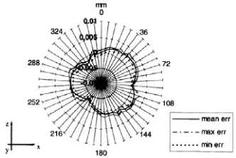
Figure 3-14. Ring gauge in a horizontal orientation on CMM (left) and scanning probe in contact with ring (right)

The ring gauge was placed on blocks in a horizontal orientation on a rotary table in Figure 3-14. The measurements at the PEC were made with the ring bolted to the spacers and in the vertical orientation. Neither measurement took advantage of the counter bore positions as kinematics supports. The scanning probe was placed in contact with the surface of the ring gauge. The gauge was rotated while the probe remained stationary. The results of the measurement are shown in Figure 3-15. The image on the left is a measurement of the swept sine wave placed on a polar axis; the right image shows the roundness of the ring with the measurement taken on the non-wave portion of the ID.

(65)

The measured swept sine wave features shown on the left in Figure 3-15 indicate a reduction in amplitude as the wave approaches its shortest length. The reduction in amplitude is both at the peak and the valley of the wave. This distortion was also apparent in the LVDT measurements at the PEC as described in Section 3.1.5.1. The measurement of roundness, right image, confirms the lobes caused by the elastic deformation created by the bolts during fabrication. The ring is out-of-round by a PV value of 3.8µm. The ring was bolted to three spacers which were shown to cause some distortion when the bolts were removed. The amplitude reduction and distortion issues must be addressed before a final artifact can be produced.

3.2 C

YLINDRICAL

A

RTIFACT

(66)

Figure 3-16. Experimental setup to machine swept sine wave on OD of cylinder and the air-bearing LVDT used to measure the final shape

The cap gage output for the swept sine wave is shown in Figure 3-17, and it indicates an increase in displacement at the highest frequencies. This is consistent with the open loop characteristics of the FTS in Figure 3-4. However, a measurement of these same sine wave features shown in Figure 3-17 using the air-bearing LVDT exhibited the same features measured on the original ring gauge; that is, reduced amplitude at the higher frequencies. The discontinuity in the amplitude near the lowest frequencies is due to no features present rather than measurement error.

(67)

To verify the output of the cap gage, the output from the high voltage (HV) amplifier before it was sent to the FTS was monitored on an oscilloscope. The intention was to determine whether the amplifier had the same gain over the frequency range of interest.

Figure 3-18. Swept sine wave output thru the HV amplifier as seen on an oscilloscope Figure 3-18 illustrates the response of the amplifier. It is apparent that at the higher frequencies, the voltage increases as it is sent into the FTS. The peak-to-peak voltage measures 3.36V, which translates to 5.34µm of displacement. At the lower frequency section, the peak-to-peak voltage measures 3.11V or 4.93µm. The HV amplifier is adding its own dynamics to the system that is affecting the desired swept sine wave input.

3.2.1 Sources of Error

The difference between the cap gauge reading and the LVDT was either due to fabrication or measurement. Several hypotheses were proposed and tested; they included tool clearance, size of LVDT probe tip diameter, LVDT electronics, and actual surface features.

3.2.1.1 Tool Clearance

(68)

wavelength (highest frequency) is greater than the clearance angle of the tool, portions of the wave could be cut off. Equation (4) calculates the maximum slope of the swept sine wave.

Clearance angle

ψ

Clearance angle

ψ

Figure 3-19. Chip formation during machining with associated angles [23]

( )

_L A

Slope_max = * 2π (4)

where:

A = Amplitude of the wave (0.0025mm)

L = Minimum wavelength (0.317mm)

The maximum slope is 0.05 radian or 2.84˚ with the proposed values. On the cylinder, the shortest wavelength measured 0.186mm and 0.287mm on the ring gauge. This translates to 4.84˚ and 3.14˚, respectively. Even though the shortest wavelength was shorter than desired, the waves are not cut off at the highest frequencies by the tool. 3.2.1.2 Probe Tip Diameter

(69)

Figure 3-20. Probe compensation concept [20]

Figure 3-20 (image not to scale) demonstrates the concept behind probe compensation. The LVDT probe measures the wave as the part rotates on the DTM spindle. The measurement data contains the position of the center of the probe rather than the probe’s position on the surface of the wave; the probe compensation equations find the surface position. The radius is measured from the center of the part where the probe is shown on the outside surface of the cylinder. The equations of the probe compensation are shown in Equations (5-7) with r as the radius of the probe [20].

     ₋ = − θ ρ ρ φ d d 1

tan 1 ₍₅₎

φ ρ ρ

ρ'₌ 2 ₊_r2 ₋2 _rcos ₍₆₎

( )

φ θ ρ θ _+      − =_sin− _sin

(70)

Valley Peak

Figure 3-21. Top subplot is the expected measurement and bottom is actual LVDT measurement

The probe compensated data in the top subplot of Figure 3-21 showed that the LVDT probe could not measure the valleys of the wave (the absent triangular sections) but indicated that all the peaks could be measured. This may be attributed to a shorter than desired spatial wavelength (as discussed in Section 3.2.1.1) that prevented the probe from fitting into the valley of the wave. The reduction of the peak, at the top of the bottom subplot, at the shortest spatial wavelengths (0.187mm or 28Hz with 1RPM measurement speed) is due to the filtering of the instrument when the probe lost contact with the surface after not being able to properly measure the valleys (refer to Figure 4-5 in Section 4.4.1 for the LVDT dynamics). The compensation equations do not take into account the speed of measurement and assume exact following of the wave.

3.2.1.3 LVDT Calibration

Metrology Artifact Design

ABSTRACT

METROLOGY ARTIFACT DESIGN

BIOGRAPHY

ACKNOWLEDGEMENTS

TABLE OF CONTENTS

LIST OF FIGURES

LIST OF TABLES

1

INTRODUCTION

1.1

H

1.1.1

Rotary Contour Gage

1.1.2

Coordinate Measuring Machines (CMMs)

1.1.3

Probes

1.2

E

T

R

M

E

1.2.1

Error Map

1.2.2

Calibrated Artifacts

1.3

D

O

2

ARTIFACT DEVELOPMENT

2.1

R

G

S

2.1.1

Material

2.2

R

G

S

F

2.3

D

A

T

2.3.1

Discrete Fourier Transform (DFT)

∑

2.3.2

Single Frequency Sine Wave

2.3.3

Multiple Single Frequency Sine Waves

2.3.4

Concatenation of Waves

2.3.5

Swept Sine Wave

3

ARTIFACT FABRICATION

3.1

A

A

3.1.1

Machining Ring Structure

3.1.2

Swept Sine Wave Machining Process Development

20 RPM

Shortest

Waves

Longest

Waves

Shortest

Waves

Longest

Waves

3.1.3

FTS Open Loop Control

3.1.4