INVESTIGATION
Positional Information, Positional Error, and
Readout Precision in Morphogenesis: A
Mathematical Framework
Gasper Tkaˇ cik,*ˇ ,1Julien O. Dubuis,†,‡Mariela D. Petkova,†and Thomas Gregor†,‡
*Institute of Science and Technology Austria, A-3400 Klosterneuburg, Austria, and†Joseph Henry Laboratories of Physics and‡Lewis Sigler Institute for Integrative Genomics, Princeton University, Princeton, New Jersey 08544
ABSTRACTThe concept of positional information is central to our understanding of how cells determine their location in a multi-cellular structure and thereby their developmental fates. Nevertheless, positional information has neither been defined mathematically nor quantified in a principled way. Here we provide an information-theoretic definition in the context of developmental gene ex-pression patterns and examine the features of exex-pression patterns that affect positional information quantitatively. We connect positional information with the concept of positional error and develop tools to directly measure information and error from experimental data. We illustrate our framework for the case of gap gene expression patterns in the earlyDrosophilaembryo and show how information that is distributed among only four genes is sufficient to determine developmental fates with nearly single-cell resolution. Our approach can be generalized to a variety of different model systems; procedures and examples are discussed in detail.
C
ENTRAL to the formation of multicellular organisms isthe ability of cells with identical genetic material to acquire distinct cell fates according to their position in a de-veloping tissue (Lawrence 1992; Kirschner and Gerhart 1997). While many mechanistic details remain unsolved, there is a wide consensus that cells acquire knowledge about their location by measuring local concentrations of various
form-generating molecules, called “morphogens” (Turing
1952; Wolpert 1969). In most cases, these morphogens di-rectly or indidi-rectly control the activity of other genes, often coding for transcription factors, resulting in a regulatory
network whose successive layers produce refined spatial
pat-terns of gene expression (von Dassowet al.2000; Tomancak
et al.2007; Fakhouriet al.2010; Jaeger 2011). The system-atic variation in the concentrations of these morphogens with
position defines a chemical coordinate system, used by cells
to determine their location (Nüsslein-Volhard 1991; St.
Johnston and Nüsslein-Volhard 1992; Grossniklaus et al.
1994). Morphogens are thus said to contain “positional
in-formation,”which is processed by the genetic network,
ulti-mately giving rise to cell fate assignments that are very re-producible across the embryos of the same species (Wolpert 2011).
The concept of positional information has been widely used as a qualitative descriptor and has had an enormous success in shaping our current understanding of spatial
pat-terning in developing organisms (Wolpert 1969; Tickleet al.
1975; French et al. 1976; Driever and Nüsslein-Volhard
1988a,b; Meinhardt 1988; Struhl et al.1989; Reinitzet al.
1995; Schier and Talbot 2005; Ashe and Briscoe 2006; Jaeger
and Reinitz 2006; Bökel and Brand 2013; Witchleyet al.
2013). Mathematically, however, positional information has
not been rigorously defined. Specific morphological features
during early development have been studied in great detail and shown to occur reproducibly across wild-type embryos
(Gierer 1991; Gregoret al.2007a; Gregoret al.2007b;
Okabe-Oho et al.2009; Dubuiset al.2013a; Liuet al.2013), while perturbations to the morphogen system resulted in systematic shifts of these same features (Driever and Nüsslein-Volhard 1988a,b; Struhlet al.1989; Liuet al.2013). This established a causal—but not quantitative—link between the positional in-formation encoded in the morphogens and the resulting body plan.
InDrosophila, the body plan along the major axis of the future adultfly is established by a hierarchical network of
inter-acting genes during the first 3 hr of embryonic development
Copyright © 2015 by the Genetics Society of America doi: 10.1534/genetics.114.171850
Manuscript received April 22, 2014; accepted for publication October 27, 2014; published Early Online October 31, 2014.
(Nüsslein-Volhard and Wieschaus 1980; Akam 1987; Ingham 1988; Spradling 1993; Papatsenko 2009). The hierarchy is composed of three layers: long-range protein gradients that span the entire long axis of the egg (Driever and Nüsslein-Volhard, 1988a), gap genes expressed in broad bands (Jaeger 2011), and pair-rule genes that are expressed in a regular seven-striped pattern (Lawrence and Johnston 1989). Posi-tional information is provided to the system solely via thefirst layer, which is established from maternally supplied and highly localized messenger RNAs (mRNAs) that act as protein sources for the maternal gradients (Nüsslein-Volhard 1991;
St. Johnston and Nüsslein-Volhard 1992; Ferrandon et al.
1994; Anderson 1998; Littleet al.2011). The network uses
these inputs to specify a blueprint for the segments of the
adultfly in the form of gene expression patterns that
cir-cumferentially span the embryo in the transverse
direc-tion to the anterior–posterior axis. These patterns define
distinct single-nucleus wide segments with nuclei expressing the downstream genes in unique and distinguishable combi-nations (Gergenet al.1986; Gregoret al.2007a; Dubuiset al. 2013a,b).
It is remarkable that such precision can be achieved in such a short amount of time, using only a few handfuls of
genes. Gene expression is subject to intrinsic fluctuations,
which trace back to the randomness associated with regula-tory interactions between molecules present at low absolute copy numbers (van Kampen 2011; Tsimring 2014). Moreover, there is random variability not only within, but also between, embryos, for instance in the strength of the morphogen sources (Bollenbachet al.2008). These biophysical limitations—e.g., in the number of signaling molecules, the time available for morphogen readout, and the reproducibility of initial and
environmental conditions—place severe constraints on the
ability of the developmental system to generate
reproduc-ible gene expression patterns (Gregor et al. 2007a; Tkaˇcik
et al.2008).
Given these constraints, how precisely can gene expression levels encode information about position in the embryo? To address this question rigorously, we need to be able to make quantitative statements about the positional information of
spatial gene expression profiles without presupposing which
features of the profile (e.g., sharpness of the boundary, size of the domains, position-dependent variability, etc.) encode the information. Here we make the case that the relevant
mea-sure for positional information is themutual information
I—a central information-theoretic quantity (Shannon 1948)—
between expression profiles of the gap genes and position
in the embryo. We show how positional information puts mathematical limits on the ability with which cells in the
developingDrosophila embryo can infer their position along
the major axis by simultaneously reading the concentrations of multiple gap gene proteins. This framework allows us (i) to quantitatively determine how many truly distinct and
mean-ingful levels of gene expression are generated by the
Drosoph-ilagap gene system, (ii) to assess how many distinguishable
cell fates such a system can support, and (iii) to ask how
variability across embryos impedes the ability of the pattern-ing system to transmit positional information.
This study builds on two previously published articles. In
Dubuiset al.(2013a), the general data acquisition and error
analysis frameworks were presented with a subset of the data analyzed here (referred to as data set A below); here we analyze roughly eight times as many samples, to assess the experimental reproducibility of the results and perform tests that would be impossible with the original small
sam-ple. In Dubuiset al.(2013b), data set A was used to estimate
positional information and positional error, as outlined in greater detail here. The study aimed at understanding
posi-tional information in theDrosophilagap gene network, but
the treatment of the conceptual and data analysis frame-works was very cursory. In the present methodological arti-cle, we provide a full account of both frameworks and include a number of previously unreported results, relating to (i) the mathematical connection between positional error and information, (ii) different estimators of information from data, (iii) various data normalization techniques, (iv) com-bining data from multiple experiments, and (v) the validity of various approximation schemes. We report on these techniques in detail and benchmark them on real data to prepare our approach for a straightforward generalization to other devel-opmental systems.
Results
Theoretical foundations
In this section we establish the information-theoretic frame-work for positional information carried by spatial patterns of gene expression. To develop an intuition, we start with a one-dimensional toy example of a single gene, which will be generalized later to a many-gene system. We present scenarios where positional information is stored in different qualitative features of gene expression patterns. To capture that intuition mathematically, we give a precise definition of positional information for one and for multiple genes. Finally, we show how a quantitative formulation of posi-tional information is related to“decoding,”i.e., the ability of the nuclei to infer their position in the embryo.
Positional information in spatial gene expression profiles:
Let us consider the simplest possible example where the expression of a single geneG(x) varies with positionxalong the axis of a one-dimensional embryo. We choose units of
length such thatx= 0 andx= 1 correspond to the anterior
and posterior poles of the embryo, respectively. Suppose we
are able to quantitatively measure the profile of such a gene
along the anterior–posterior axis inNembryos, labeled with
an indexm¼1;. . .;N. Such measurements of the light
in-tensity profile of fluorescently labeled antibodies against
a particular gene product yieldG(m)(x), whereGis the
quan-titative readout in embryo m of the gene expression level.
From a collection of embryos—after suitable data processing
position-dependent “mean profile,”capturing the prototyp-ical gene expression pattern, and the position-dependent variance across embryos, which measures the degree of embryo-to-embryo variability or the reproducibility of the mean
profile. We can transform the measurementsG(x) into
pro-filesg(x) with rescaled units, such that the mean profilegðxÞ is normalized to 1 at the maximum and to 0 at the minimum alongx. After these steps, our description of the system consists of the mean profile,gðxÞ;and the variance in the profile,sg2ðxÞ:
How much can a nucleus learn about its position if it
expresses a gene at level g? We compare three idealized
cases, where we pick the shape ofgðxÞby hand and assume,
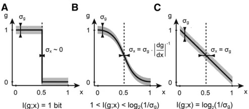
for the start, that the variance is constant, sg2ðxÞ ¼c: The first case is illustrated in Figure 1A, where a step-like profile
ingsplits the embryo into two domains of gene expression:
an anterior“on”domain, wheregðxÞ ¼1 forx,x0, and an “off”domain in the posterior,x.x0, wheregðxÞ ¼0:This
arrangement has an extremely precise, indeed infinitely
sharp, boundary at x0; if we think that the sharpness of
the boundary is the biologically relevant feature in this sys-tem, this arrangement would correspond to an ideal pattern-ing gene. But how much information can nuclei extract from
such a profile? If x0 were 1/2, the boundary would
repro-ducibly split the embryo into two equal domains: based on
reading out the expression of g, the nucleus could decide
whether it is in the anterior or the posterior, a binary choice that is equally likely prior to reading outg. As we will see, the positional information needed (and provided by such
a sharp profile!) to make a clear two-way choice between
twoa prioriequally likely possibilities = 1 bit.
Can a profile of a different shape do better? Figure 1B
shows a somewhat more realistic sigmoidal shape that has a steep, but not infinitely sharp, transition region. If the
var-iance is small enough, s2
g 1;this profile can be more
in-formative about the position. Nuclei far at the anterior still haveg1 (full induction or the on state), while nuclei at the
posterior still have g0 (the off state). But the graded
re-sponse in the middle defines new expression levels ingthat
are significantly different from both 0 and 1. A nucleus with
g0.5 will thus“know”that it is neither in the anterior nor in the posterior. This system will therefore be able to provide more positional information than the sharp boundary that is limited by 1 bit. Clearly, this conclusion is valid only insofar as the variances2
g is low enough; if it gets too big, the
interme-diate levels of expression in the transition region can no lon-ger be distinguished and we are back to the 1-bit case.
In contrast to the infinitely sharp gradient, a linear gra-dient, as depicted in Figure 1C, has already been proposed as
efficient in encoding positional information (Wolpert 1969).
By extending the argument for sigmoidal shapes above, ifs2
g
is not a function of position, the linear gradient is in fact the optimal choice. Consider starting at the anterior and moving
toward the posterior: as soon as we move far enough inxthat
the change in gðxÞ is above sg, we have created one more
distinguishable level of expression in gand thus a group of
nuclei that, by measuringg, can differentiate themselves from
their anteriorly positioned neighbors. Finally, this reasoning gives us a hint about how to generalize to the case where the variance s2g depends on position,x. What is important is to
count, asxcovers the range from anterior to posterior, how
muchgðxÞ changesin units of the local variability, sg(x)—it
will turn out that this is directly related to the mutual
infor-mation betweengand position.
Thus a sharp and reproducible boundary can correspond
to a profile that does not encode a lot of positional
infor-mation, and a linear profile where the boundary is not even
well defined can encode a high amount of positional
in-formation. Ultimately, whether or not there are intermediate distinguishable levels of gene expression depends on the variability in the profile. Therefore, any measure of positional informationmustbe a function of bothgðxÞands2
gðxÞ:
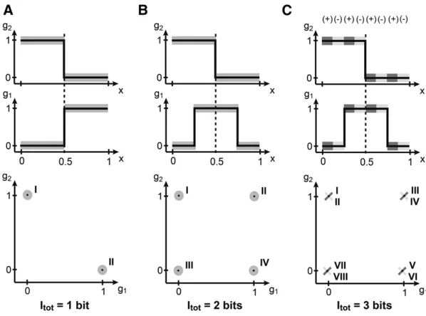
Does the ability of the nuclei to infer their position automatically improve if they can simultaneously read out the expression levels of more than one gene? Figure 2A shows the case where two genes,g1andg2, do not provide any more
information than each one of them provides separately, be-cause they are completely redundant. Redundant does not
mean equal—indeed, in Figure 2A the profiles are different
at everyx—but they are perfectly correlated (or dependent):
knowing the expression level of g1, one knows exactly the
level ofg2, sog2cannot provide any additional new information
about the position. In general, redundancy can help compen-sate for detrimental effects of noise when noise is significant, but this is not the case in the toy example at hand.
The situation is completely different if the two profiles
are shifted relative to each other by, say, 25% embryo length.
Note that none of the individual profile properties have
changed; however, the two genes now partition the embryo into four different segments: the posteriormost domain that is combinatorially encoded by the gene expression pattern g1¼g2¼0;the third domain withg1¼0; g2¼1;the
sec-ond domain withg1¼g2¼1;and the anteriormost domain
withg1¼1; g2¼0:Upon reading outg1andg2, a nucleus,
a priorilocated in any of the four domains, can unambigu-ously decide on a single one of the four possibilities. This is equivalent to making two binary decisions and, as we will later show, to 2 bits of positional information.
Finally, the most subtle case is depicted in Figure 2C.
Here, the mean profiles have exactly the same shapes as in
Figure 2B. What is different, however, is the correlation
structure of thefluctuations. In certain areas of the embryo
the two genes are strongly positively correlated, while in the others they are strongly negatively correlated. If these areas
are overlaid appropriately on top of the domains defined
by the mean expression patterns, an additional increase in positional information is possible. In the admittedly con-trived but pedagogical example of Figure 2C, the mean
pro-files and the correlations together define eight distinguishable domains of expression, combinatorially encoded by two genes. Nuclei, having simultaneous access to the concentrations of the two genes, can compute which of the eight domains they re-side in, although it might not be easy to implement such a com-putation in molecular hardware. Picking one of eight choices corresponds to making three binary decisions, and thus to 3 bits of positional information. Note that in this case, each gene considered in isolation still carries 1 bit as before, so that the system of two genes carries more information than the sum of its parts—such a scheme is called synergistic encoding.
In sum, we have shown that the mean shapes of the profiles, as well as their variancesandcorrelations, can carry positional information. Extrapolating to three or more genes, we see that the number of pairwise correlations increases and in addition higher-order correlation terms start appearing. For-mally, positional information could be encoded in all of these features, but would become progressively harder to extract using plausible biological mechanisms. Nevertheless, a princi-pled and assumption-free measure should combine all statisti-cal structure into a single number, a sstatisti-calar quantity measured
in bits, that can“count”the number of distinguishable expres-sion states (and thus positions), as illustrated in the examples above.
Defining positional information:Determining the number
of“distinguishable states”of gene expression is more
com-plicated in real data sets than in our toy models: the mean
profiles have complex shapes and their (co)variability
depends on position. In the ideal case we can measure joint expression patterns ofNgenes {gi},i= 1,. . .,N(for
exam-pleN= 4 for four gap genes inDrosophila) in a large set of
embryos. In such a scenario the position dependence of the expression levels can be fully described with a conditional probability distribution P({gi}|x). Concretely, for every
po-sitionxin the embryo we construct anN-dimensional
histo-gram of expression levels across all recorded embryos, which (when normalized) yields the desiredP({gi}|x). This
distribution contains all the information about how expres-sion levels vary across embryos in a position-dependent fashion. For instance,
giðxÞ ¼
Z
dNg giP
fglgjx; (1)
s2 iðxÞ ¼
Z
dNgðgi2giðxÞÞ2PðfglgjxÞ; (2)
CijðxÞ ¼ Z
dNg
gigj2giðxÞgjðxÞ
PðfglgjxÞ (3)
are the mean profile of genegi, the variance across embryos of
gene gi, and the covariance between genesgiand gj,
respec-tively. In principle, the conditional distribution contains also all higher-order moments that we can extract by integrating over appropriate sets of variables. Realistically, we are often limited in our ability to collect enough samples to constructP({gi}|x)
by histogram counts, especially when considering several
Figure 2 (A–C) Positional information encoded by two genes. Spatial gene expression profiles are shown at the top; an enumeration of all distinguishable combinations of gene expression (roman numerals) across the embryo is shown at the bottom. (A) Step function profiles ofg1,g2 each encode 1 bit of information, but are perfectly redun-dant, jointly encoding only two distinguishable states and thus 1 bit of positional information, the same as each gene alone. (B) The mean profiles ofg1,g2have been displaced, removing the redundancy and bringing the total informa-tion to 2 bits (four distinct states of joint gene expression). (C) If in addition to the mean profile shape the down-stream layer can read out the (correlated)fluctuations of
genes simultaneously; the number of samples needed grows exponentially with the number of genes. However, estimating the mean profiles on the left-hand sides of Equations 1–3 can
often be achieved from data directly. A reasonable first step
(but one that has to be independently verified) is to assume
that the joint distributionP({gi}|x) ofNexpression levels {gi}
at a given position x is Gaussian, which can be constructed
using the measured mean values and covariances:
PðfgigjxÞ
¼ ð2pÞ2N=2jCðxÞj21=2
3exp
2
421
2
XN
i;j¼1
ðgi2giðxÞÞ
C21ðxÞij
gj2gjðxÞ
3
5:
(4)
We emphasize that the Gaussian approximation is not
re-quired to theoretically define positional information, but it
will turn out to be practical when working with experimen-tal data; in the cases of one or two genes it is often possible to proceed without making this approximation, which pro-vides a convenient check for its validity.
While the conditional distribution, P({gi}|x), captures
the behavior of gene expression levelsat a given x, establish-ing how much information, in total, the expression levels carry about position requires us to know also how frequently
each combination of gene expression levels, {gi}, is used
across all positions. Recall, for instance, that our arguments related to the information encoded in patterns in Figure 2 rested on counting how often a pair of genes will be found in expression states 00, 01, 10, and 11 across allx. This global structure is encoded in the total distribution of expression levels, which can be obtained by averaging the conditional distribution over all positions,
PgðfgigÞ ¼ D
PfgigjxE
x¼
Z 1
0
dx PðfgigjxÞ; (5)
wherehixdenotes averaging overx. Note that we can think
of Equation 5 as a special case of averaging with a position-dependent weight,
PgðfgigÞ ¼ Z
d x PxðxÞPðfgigjxÞ; (6)
wherePx(x) is chosen to be uniform. As we shall see, in the
case ofDrosophilaanterior–posterior (AP) patterning,Px(x)
will be the distribution of possible nuclear locations along the AP axis, which indeed is very close to uniform.
When formulated in the language of probabilities, the
relationship between the positionxand the gene expression
levels can be seen as a statistical dependency. If we knew
this dependency were linear, we could measure it using,e.g.,
a linear correlation analysis between xand {gi}. Shannon
(1948) has shown that there is an alternative measure of total statistical dependence (not just of its linear component),
called the mutual information, which is a functional of the
probability distributionsPx(x) andP({gi}|x), and is defined by
Iðx/fgigÞ
¼
R
d x PxðxÞR
dNg PðfgigjxÞlog2PðfgigjxÞ PgðfgigÞ:
(7)
This positive quantity, measured in bits, tells us how much one can know about the gene expression pattern if one knows the position,x. It is not hard to convince oneself that the mutual information is symmetric; i.e.,I({gi}/ x) = I
(x/ {gi}) =I({gi}; x). This is very attractive: we do the
experiments by sampling the distribution of expression lev-els given position, while the nuclei in a developing embryo
implicitly solve the inverse problem—knowing a set of gene
expression levels, they need to infer their position. A funda-mental result of information theory states that both
prob-lems are quantified by the same symmetric quantity, the
information I({gi}; x). Furthermore, mutual information is
not just one out of many possible ways of quantifying the total statistical dependency, but rather the unique way that
satisfies a number of basic requirements, for example that
information from independent sources is additive (Shannon 1948; Cover and Thomas 1991).
The definition of mutual information in Equation 7 can be
rewritten as a difference of two entropies,
Iðfgig;xÞ ¼SPgðfgigÞ2DS½PðfgigjxÞE
x; (8)
whereS[p(x)] is the standard entropy of the distributionp(x) measured in bits (hence log base 2):
S½pðxÞ ¼ 2 Z
d x pðxÞlog2pðxÞ: (9)
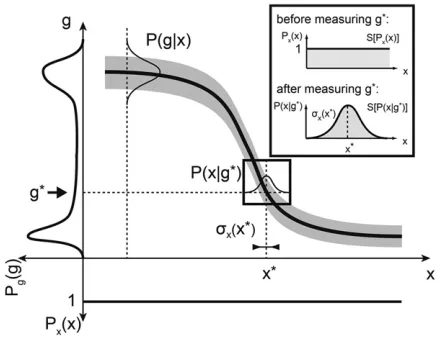
Equation 8 provides an alternative interpretation of the mutual informationI({gi};x), which is illustrated in Figure 3.
In the case of a single geneg, the“total entropy”S[Pg(g)],
represented on the left, measures the range of gene expres-sion available across the whole embryo. This total entropy, or dynamic range, can be written as the sum of two
contri-butions. One part is due to the systematic modulation ofg
with positionx, and this is the useful part (the“signal”) or the mutual informationI({gi};x). The other contribution is
the variability ingthat remains even at constant positionx; this represents pure“noise”that carries no information about posi-tion and is formally measured by the average entropy of the conditional distribution (the noise entropy), hS[P(g|x)]ix. Po-sitional information carried bygis thus the difference between the total and noise entropies, as expressed in Equation 8.
Mutual information is theoretically well founded and is always nonnegative, being 0 if and only if there is no statistical dependence of any kind between the position
and the gene expression level. Conversely, if there are I
expression patterns that can be generated by moving
along the AP axis, from the head at x = 0 to the tail at
x= 1. This is precisely the property we require from any
suitable measure of positional information. We therefore suggest that, mathematically, positional information
should be defined as the mutual information between
ex-pression level and position,I({gi};x).
Defining positional error: Thus far we have discussed positional information in terms of the statistical dependency and the number of distinguishable levels of gene expression along the position coordinate. To present an alternative interpretation, we start by using the symmetry property of the mutual information and rewriteI({gi};x) as
Iðfgig;xÞ ¼S½PxðxÞ2
S½PðxjfgigÞ PgðfgigÞ; (10)
i.e., the difference between the (uniform) distribution over
all possible positions of a cell in the embryo and the distri-bution of positions consistent with a given expression level. Here, P(x|{gi}) can be obtained using Bayes’rule from the
known quantities:
PðxjfgigÞ ¼PðfgigjxÞPxðxÞ PgðfgigÞ :
(11)
The total entropy of all positions,S[Px(x)] in Equation 10, is
independent of the particular regulatory system—it simply
measures the prior uncertainty about the location of the cells in the absence of knowing any gene expression level. If, however, the cell has access to the expression levels of a particular set of genes, this uncertainty is reduced, and it is hence possible to localize the cell much more precisely; the reduction in uncer-tainty is captured by the second term in Equation 10. This form of positional information emphasizes thedecoding view, that is, that cells can infer their positions by simultaneously reading out protein concentrations of various genes (Figure 3).
Positional information is a single number: it is a global measure of the reproducibility in the patterning system. Is there a local quantity that would tell us, position by position, how well cells can read out their gene expression levels and
infer their location? Is positional information “distributed
equally” along the AP axis or is it very nonuniform, such
that cells in some regions of the embryo are much better at reproducibly assuming their roles?
The optimal estimator of the true locationxof a cell, once
we (or the cell) measure the gene expression levels fg*
ig;
is the maximum a posteriori (MAP) estimate, x*ðfg*
igÞ ¼
argmax Pðxjfg*
igÞ:In cases like ours, where the prior
distri-butionPx(x) is uniform, this equals the maximum-likelihood
(ML) estimate,
x*ng* i
o
¼argmax Png* iox
; (12)
thus, for each expression level readout, this“decoding rule” gives us the most likely position of the cell, x*. The inset in Figure 3 illustrates the decoding in the case of one gene.
How well can this (optimal) rule perform? The expected
error of the estimated x* is given by s2
xðx*Þ ¼
ðx2x*Þ2 ;
where brackets denote averaging overPðxjfg*
igÞ:This error
is a function of the gene expression levels; however, we can
also evaluate it for everyx, since we know the mean gene
expression profiles,giðxÞ;for everyx. Thus, we define a new
quantity, the positional error sx(x), which measures how
well cells at a true positionxare able to estimate their position based on the gene expression levels alone. This is the local measure of positional information that we were aiming for.
Independently of how cells actually read out the concen-trations mechanistically, it can be shown that sx(x) cannot
be lower than the limit set by the Cramer–Rao bound (Cover
and Thomas 1991),
sx2ðxÞ$
1
IðxÞ; (13)
whereIðxÞis the Fisher information given by
IðxÞ ¼ 2
@2logPðfgigjxÞ @x2
PðfgigjxÞ:
(14)
Despite its name, the Fisher informationIis not an
information-theoretic quantity, and unlike the mutual informationI, the
Fisher information depends on position. Is there a connection
between the positional error, sx(x), and the mutual
infor-mationI({gi};x)? Below we sketch the derivation, following Figure 3 The mathematics of positional information and positional error
for one gene. The mean profile of geneg(thick solid line) and its vari-ability (shaded envelope) across embryos are shown. Nuclei are distrib-uted uniformly along the AP axis;i.e., the prior distribution of nuclear positionsPx(x) is uniform (shown at the bottom). The total distribution of expression levels across the embryo,Pg(g), is determined by averaging P(g|x) over all positions and is shown on the left. The positional information
I(g;x) is related to these two distributions as in Equation 8. Inset shows decoding (i.e., estimating) the position of a nucleus from a measured expression levelg*. Prior to the“measurement”all positions are equally likely. After observing the value g*, the positions consistent with this measured values are drawn fromP(x|g*). The best estimate of the true position,x*, is at the peak of this distribution, and the positional error,
Brunel and Nadal (1998), demonstrating the link for the case of one gene,g.
Let us assume that the Gaussian approximation of Equa-tion 4 holds and that the distribuEqua-tion of the levels of a single gene at a given position is
PðgjxÞ ¼ ffiffiffiffiffiffiffiffiffiffiffiffiffiffiffiffiffiffi1 2ps2
gðxÞ
q exp
(
21
2
ðg2gðxÞÞ2
s2 gðxÞ
)
: (15)
We can use the Gaussian distribution to compute the Fisher
information in Equation 14. Wefind that
I ¼g92ðxÞ s2
gðxÞ þ2s9
2 gðxÞ s2
gðxÞ
; (16)
where ()9denotes a derivative with respect to position,x. Information about position is thus carried by the change in
mean profile with position, as well as the change in the
var-iability itself with position. If the noise is small,sgg;then
typically it will be the case that sg9 jg9j (a potentially
important issue arises when the profiles and their variability are estimated from noisy sampled data; in this case one needs to be careful about spurious contributions to Fisher
information due to noise-induced gradients of the profiles
and the variability). If we formally require sg9 jg9j; we
can retain only thefirst term to obtain a bound on positional
error:
s2 xðxÞ$
1
IðxÞ
dg d x
22
s2
gðxÞ: (17)
This result is intuitively straightforward: it is simply the transformation of the variability in gene expression,s2
gðxÞ;into
an effective variance in the position estimate,s2
xðxÞ;and the
two are related by slope of the input/output relation,gðxÞ:
A crucial next step is to think ofxas determining gene
expressionsgiprobabilistically, and thex* as being a function
of these gene expression levels—that is, when computingx*
neither we nor the nuclei have access to the true position.
This forms a dependency chain,x/{gi}/x*. Since each
of these steps is probabilistic, it can only lose information, such that by information-processing inequality (Cover and Thomas 1991) we must haveI({gi};x)$I(x*;x). The
mu-tual information between the true location and its estimate is given by
Iðx*;xÞ ¼S½Pxðx*Þ2 D
S½Pðx*jxÞ E
PxðxÞ
: (18)
Under weak assumptions, the first term in our case is
ap-proximately the entropy of a uniform distribution. While we
do not know the full distribution P(x*|x) and thus cannot
compute its entropy directly, we know its variance, which is just the square of the positional error, s2
xðxÞ:Regardless of
what the full distribution is, its entropy must be less or equal
to the entropy of the Gaussian distribution of the same var-iance, which isS½Pðx*jxÞ ¼log2
ffiffiffiffiffiffiffiffiffiffiffiffiffiffiffiffiffiffiffiffi 2pes2
xðxÞ
p
bits. Putting
ev-erything together, wefind that
Iðfgig;xÞ$Iðx*;xÞ$ *
log2
PxðxÞ ffiffiffiffiffiffiffiffiffiffiffiffiffiffiffiffiffiffiffiffi 2pes2
xðxÞ
p
+
x
: (19)
Therefore, positional information I({gi}; x) puts an upper
bound to the average ability of the cells to infer their loca-tions, that is, to the smallness of the positional errorsx(x).
In a straightforward generalization of a single-gene case, the Fisher information for a multivariate Gaussian distribution, written for compactness in matrix notation, yields
I ¼g9TC21g9þ1
2Tr h
C21C9C21C9i: (20)
Under the same assumptions we made for the case of a single gene, we retain only thefirst term, so that the expression for positional error, written out explicitly in the component notation, reads
s2 xðxÞ$
1
IðxÞ 0
@XN
i;j¼1
dgi
d x h
CðxÞ21 i ij dgj dx 1 A 21 ; (21)
whereCijis the covariance matrix of the profiles, as defined
in Equation 3. This extends the fundamental connection, Equation 19, between the positional information and posi-tional error, to the case of multiple genes. Importantly, all
quantities—the mean profiles and their covariance—in
Equation 21 can be obtained from experimental data, so
sx(x) is a quantity that can be estimated directly.
Interpretation in a spatially discrete (cellular) system: In the setup presented above, gene expression levels carry
information about a continuous position variable,x. But in
a real biological system, there exists a minimal spatial scale—
the scale of individual nuclei (or cells)—below which the
concept of gene expression at a position is no longer well
defined. This is particularly the case in systems that interpret molecular concentrations to make decisions that determine cell fates: such interpretations have no meaning at the spa-tial scale of a molecule, but only at cellular scales. How should positional information be interpreted in such a context?
When noise is small enough and the distribution of positions consistent with observed gene expression levels, P(x|{gi}) of Equation 11 is nearly Gaussian, and Equations
19 and 21 become tight bounds. In this case we can apply Equation 10 directly. In developmental systems, cells or nuclei are often distributed in space such that the intercel-lular (or internuclear) spacings are, to a good approxima-tion, equal: at least in systems we are studying, there are
no significant local rarefactions or overabundances of cells
or nuclei. Mathematically, this amounts to assuming that Px(x) = 1/L(whereLis the linear spatial extent over which
uniformity is not crucial for any calculation in this article and can be easily relaxed, but it makes the equations some-what simpler to display and interpret. Using a uniform dis-tribution forPx(x), the information is
Iðfgig;xÞ *
log2
L ffiffiffiffiffiffiffiffiffiffiffiffiffiffiffiffiffiffiffiffi 2pes2
xðxÞ
p
+
x
: (22)
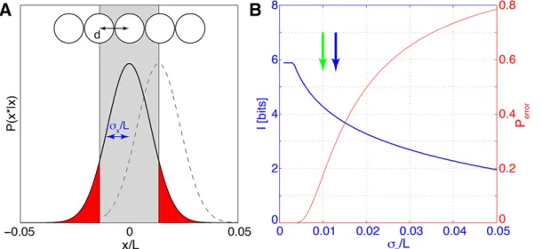
Note that in the problem setup we have normalized the spatial axis so that the lengthL= 1 in the formula above (or, if we restrict the attention to some section of the embryo, the fractional size of that section). For any real data set one needs to verify that the approximations leading to this result are warranted (see below). Assuming that, Equation 22 fur-ther illustrates the connection between positional error and positional information. Consider a one-dimensional row of
nuclei spaced by internuclear distancedalong the AP axis,
as illustrated in Figure 4. To determine its position along the
AP axis, each nucleus has to generate an estimatex* of its
true positionxby reading out gap gene expression levels. In
the simplest case, the errors of these estimates are indepen-dent, normally distributed, with a mean of zero and a vari-ance s2
x:Given these parameters, there is some probability
Perrorthat the positional estimate deviates by more than the
lattice spacingd, in which case the nucleus would be assigned to the wrong position, and perfectly unique,
nucleus-by-nucleus identifiability would be impossible. Figure 4 shows
how the positional information of Equation 22 and the proba-bility of fate misassignment, Perror, vary as functions of sx.
Importantly, even when sx , d, that is, the positional error
is smaller than the internuclear spacing (as in Figure 4A), there is still some probability of nuclear misidentification and there-fore the positional information has not yet saturated. Only when the positional error is sufficiently small that the proba-bility weight in the tails of the Gaussian distribution is
negligi-ble (at sx d), can each of the Nn nuclei be perfectly
identified and the information saturates at log2(Nn) bits.
In sum, we have shown that a rigorous mathematical framework of positional information can quantify the
repro-ducibility of gene expression profiles in a global manner. By
framing the cells’ problem of finding their location in the
embryo in terms of an estimation problem, we have shown that the same mathematical framework of positional infor-mation places precise constraints on how well the cells can infer their positions by reading out a set of genes. These constraints are universal: regardless of how complex the
mechanistic details of the cells’readout of the gene
concen-tration levels are, the expression level variability prevents
the cells from decreasing the positional error belowsx. The
concept of positional error easily generalizes to the case of multiple genes and is diagnostic about how positional infor-mation is distributed along the AP axis.
Estimation methodology
There are a number of technical details that need to be
fulfilled when applying the formalisms of positional
in-formation and positional error to real data sets. Estimating
information theoretic quantities fromfinite data is generally
challenging (Paninski 2003; Slonimet al.2005). In practice
it involves combining general theory and algorithms for
in-formation estimation with problem-specific approximations.
Here we present the information content of the four major gap genes in earlyDrosophilaembryos as a test case. First, we
briefly recapitulate our experimental and data-processing
methods (for details, see Dubuis et al. 2013a). Next, we
present the statistical techniques necessary to consistently merge data from separate pairwise gap gene immunostain-ing experiments into a simmunostain-ingle data set. Then we estimate mutual information directly from data for one gene, using
different profile normalization and alignment methods.
Fi-nally, we introduce the Gaussian noise approximation and an adaptive Monte Carlo integration scheme to extract the information carried jointly by pairs of genes and by the full set of four genes.
Extracting expression level profiles from imaging data:
Drosophila embryos were fixed and simultaneously
immu-nostained for the four major gap genes hunchback (hb),
Krüppel(Kr),knirps(kni), andgiant(gt), usingfluorescent antibodies with minimal spectral overlap, as described in
Dubuiset al.(2013a). We present an analysis of four data sets
(A, B, C, and D): data sets A–C have been processed
simulta-neously, but imaged in different sessions; data set D has been processed and imaged independently from the other data sets. Hence these datasets are well suited to assess the dependence of our measurements and calculations on the experimental processing. Dataset A has been presented and analyzed pre-viously in Dubuiset al.(2013a,b) and Krotovet al.(2013).
Fluorescence intensities were measured using automated laser scanning confocal microscopy, processing hundreds of embryos in one imaging session. Cross-sectional images of multicolor-labeled embryos were taken with an imaging focus at the midsagittal plane, the center plane of the
embryo with the largest circumference. Intensity profiles of
individual embryos were extracted along the outer edge of the embryos, using custom software routines (MATLAB; MathWorks, Natick, MA) as described in Houchmandzadeh et al. (2002) and Dubuiset al. (2013a). The results in the following sections are presented using exclusively dorsal
in-tensity profiles, and we report their projection onto the AP
axis in units normalized by the total lengthLof the embryo,
yielding a fractional coordinate between 0 (anterior) and 1 (posterior). The dorsal edge was chosen for its smaller
cur-vature, which limits geometric distortions of the profiles
when projecting the intensity onto the AP axis. The AP axis was uniformly divided into 1000 bins, and the average
pro-file intensity in each bin is reported. This procedure results
in a raw data matrix that lists, for each embryo and for each of the four gap genes, one intensity value for each of the 1000 equally spaced spatial positions along the AP axis. Un-less specified differently, all our results are reported for the
middle 80% of the AP axis (fromx= 0.1 tox= 0.9),
con-sistent with Dubuiset al.(2013b); at the embryo poles
geo-metric distortion is large, and patterning mechanisms are distinct from the middle.
For any successful information-theoretic analysis, the dom-inant source of observed variability in the data set must be due to the biological system and not due to the measure-ment process, requiring tight control over systematic mea-surement errors. Gap gene expression levels critically depend on the developmental stage and on the imaging orientation of the embryo. Therefore we applied strict selection criteria on developmental timing and orientation angle (see Dubuis et al.2013a). In this article we restrict our analysis to a time
window of10 min, 38–48 min into nuclear cycle 14.
Dur-ing this time interval the mean gap gene expression levels peak and overall temporal changes are minimal. A careful analysis of residual variabilities due to measurement error (i.
e., age determination, orientation, imaging, antibody
nonspe-cificity, spectral crosstalk, and focal plane determination)
reveals that the estimated fraction of observed variance in
the gap gene profiles due to systematic and experimental
error is ,20% of the total variance in the pool of profiles;
i.e.,.80% of the variance is due to the true biological var-iability (Dubuiset al.2013a), satisfying the condition for the information-theoretic analysis to yield true biological insight.
In most cases expression profiles need to be normalized
before they can be compared or aggregated across embryos. Careful experimental design and imaging conditions can
make normalization steps essentially superfluous (Dubuis
et al. 2013a), but such control may not always be possible. To deal with experimental artifacts, we introduce three pos-sible types of normalizations, which we call Y alignment, X alignment, and T alignment. In Y alignment, the recorded
intensity of immunostaining for each profile of a given gap
gene, G(m)(x) recorded from embryo m ðm¼1;. . .;N Þ; is assumed to be linearly related to the (unknown) true con-centration profileg(m)(x) by an additive constant am and an
overall scale factor bm (to account for the background and
staining efficiency variations from embryo to embryo,
respec-tively), so thatG(m)(x) =am+bmg(m)(x). We wish to minimize
the total deviation x2 of the concentration profiles from the
mean across all embryos. The objective function is
x2 Y
n
am;bm
o
¼XN m¼1
Z 1
0
dx
GðmÞðxÞ2 h
amþbmgðxÞ
i2
;
(23)
wheregðxÞ ¼ N21PmgðmÞðxÞdenotes an average
concentra-tion profile across allN embryos. The parameters {am,bm}
are chosen to minimize the x2
Y and thus maximize
align-ment, and since the cost function is quadratic, this
optimi-zation has a closed-form solution (Gregor et al. 2007a;
Dubuiset al.2013a).
Additionally, one can perform the X alignment, whereall
gap gene profiles from a given embryo can be translated
along the AP axis by the same amount; this introduces one
more parametergiper embryo (notper expression profile),
which can be again determined usingx2minimization,
sim-ilar to the above. (In practice, onefirst carries out the
trac-table Y alignment, followed by a joint minimization ofx2for
a,b,g, which needs to be carried out numerically.) There
are two candidate sources of variability that can be compen-sated for by X alignments: (i) our error in the exact
deter-mination of the AP axis,i.e., in the exact end points of the
embryo, due to image processing; and (ii) real biological variability that would result in all the nuclei within the em-bryo being rigidly displaced by a small amount along the long axis of the embryo relative to the egg boundary.
Finally, the T alignment attempts to compensate for the fraction of observed variability that is due to the systematic
change in gene profiles with embryo age even within the
chosen 10-min time bracket. We can use our knowledge of
how the mean profiles evolve with time and detrend the
entire data set in a given time window by this evolution of
the mean profile. We follow the procedure outlined in Dubuis
et al.(2013a) to carry out this alignment.
after alignment, successive alignment procedures should lead to increases in positional information. Strictly speaking, the lower bound on positional information would be obtained by estimating it using raw data, without any alignment, thus ascribing all variability in the recorded profiles to the true biological variability in the system, but unless the control over experimental variability is excellent, this lower bound might be far below the true value. For instance, if embryos cannot be stained and imaged in a single session, it would be very hard to guarantee that there are no embryo-to-embryo variabilities in the antibody staining and imaging background. For that reason, we view the Y alignment as the minimal procedure that should be performed unless staining and imaging variability is shown to be negligible in dedicated control experiments. The choice of performing alignments
beyond Y depends on system-specific knowledge about the
plausible sources of experimentalvs.biological variability. For these reasons, all the results in this article are based on the minimal Y alignment procedure (unless explicitly specified otherwise), thus yielding conservative information estimates, but we also explore how these estimates would increase for single genes and the quadruplet in the case of the other alignments.
Once the desired alignment procedure has been carried
out, we can define the mean expression across the embryos,
giðxÞ for every gap genei= 1,. . ., 4, and choose the units
for the profiles such that the minimum value of each mean
profile across the AP axis is 0, and the maximal value is 1.
This is the final, aligned and normalized, set of profiles on
which we carry out all subsequent analyses and from which
we compute the covariance matrixCij(x) of Equation 3.
Applying the described selection criteria to the four
mentioned data sets yields embryo counts of N ¼24 (A),
N ¼32 (B),N ¼31 (C), andN ¼102 (D). Figure 5 shows
the mean profiles and their variability for two of the data sets, using either the minimal (Y) or the full (XYT) alignment.
Estimating information with limited amounts of data:
Measuring positional information from afinite numberN of
embryos is challenging due to estimation biases. Good esti-mators are more complicated than the naive approach, which consists of estimating the relevant distributions by counting and using Equation 7 for mutual information directly. Nevertheless, the naive approach can be used as a basis for an
unbiased information estimator, following the so-called direct
method(Stronget al.1998; Slonimet al.2005).
The easiest way to obtain a naive estimate forP({gi},x) is
to convert the range of continuous values for giandxinto
discrete bins of sizeDN3D. On this discrete domain, we can
estimate the distribution P~D;Mðfgig;xÞ empirically by
creat-ing a normalized histogram. To this end, we treat our data
matrix of (4 gap genes) 3 (N embryos) 3 (1000 spatial
bins) as containing M¼10003N samples from the joint
distribution of interest. A naive estimate of the positional
information,IDIR
D;Mðfgig;xÞ;is
IDIR
D;Mðfgig;xÞ
¼ P
fgig;x
~
PD;Mðfgig;xÞlog2
~
PD;Mðfgig;xÞ e
PxD;MðxÞPegD;MðfgigÞ
; (24)
where the subscripts indicate the explicit dependence on sample sizeMand bin sizeD. It is known that naive estimators
suffer from estimation biases that scale as 1/M and DN+1.
Following Strong et al.(1998) and Slonimet al.(2005), we
can obtain adirect estimateof the mutual information byfirst computing a series of naive estimates for afixed value ofDand for fractions of the whole data set. Concretely, we pick fractions
m¼ ½0:95 0:9 0:85 0:8 0:75 0:53N of the total number of
embryos, N:At each fraction, we randomly pickmembryos
100 times and compute hIDIR
D;mðfgig;xÞi (where averages are
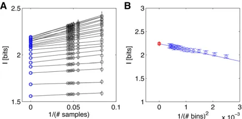
taken across 100 random embryo subsets). This gives us a se-ries of data points that can be extrapolated to an infinite data limit by linearly regressinghIDIR
D;mðfgig;xÞivs.1/m(Figure 6A).
The intercept of this linear model yieldsIDIR
D;m/Nðfgig;xÞ, and we can repeat this procedure for a set of ever smaller bin sizes
D. To extrapolate the result to very small bin sizes,D/0, we
use the previously computedIDIR
D;N;ðfgig;xÞfor various choices
of decreasingD, and extrapolate toD/0 as shown in Figure
6B. At the end of this procedure we obtain thefinal estimate
IDIR
D/0;n/Nðfgig;xÞ; called direct estimate (DIR) of positional information (red square in Figure 6B). While no prior knowl-edge about the shape of the distributionP({gi},x) is assumed
by the direct estimation method, a potential disadvantage is the amount of data required, which grows exponentially in the number of gap genes. In practice, our current data sets suffice for the direct estimation of positional information carried si-multaneously by one or at most two gap genes.
To extend this method tractably to more than two genes,
one needs to resort to approximations forP({gi}|x), the
simplest of which is the so-called Gaussian approximation, shown in Equation 4. In this case, we can write down the entropy ofP({gi}|x) analytically. For a single gene we get
S~PD;MðgjxÞ
¼1
2log2
2pes2gðxÞ
þlogD; (25)
while the straightforward generalization to the case of N
genes is given by
S~PD;MðfgigjxÞ¼1 2log2
ð2peÞNCðxÞþNlogD; (26)
where |C(x)| is the determinant of the covariance matrix
Cij(x). From Equation 8 we know thatI(g;x) =S[P(g)]2 hS[P(g|x)]ix. Here the second term (“noise entropy”) is therefore easily computable from Equation 25, for a
discretized version of the distribution, P~; using the (co)
variance estimate of gene expression levels alone. Thefirst
term (total entropy) can be estimated as above by the
direct method, i.e., by making an empirical estimate of
~
PD;MðgÞ for various sample sizesMand bin sizes Dand
ex-trapolating M/N andD/0. This combined procedure,
where we evaluate one term in the Gaussian approxima-tion and the other one directly, has two important proper-ties. First, the total entropy is usually much better sampled than the noise entropy, because it is based on the values of
gpooled together over every value ofx; it can therefore be
estimated in a direct (assumption-free) way even when the noise entropy cannot be. Second, by making the Gaussian
approximation for the second term, we are always
overes-timating the noise entropy and thus underestimating the total positional information, because the Gaussian distribu-tion is the maximum entropy distribudistribu-tion with a given
mean and variance. Therefore, in a scenario where thefirst
term in Equation 25 is estimated directly, while the second term is computed analytically from the Gaussian ansatz, we always obtain a lower bound on the true positional infor-mation. We call this bound (which is tight if the conditional
distributions really are Gaussian) thefirst Gaussian
approx-imation (FGA).
For three or more gap genes the amount of data can be insufficient to reliably apply either the direct estimate or FGA, and one needs to resort to yet another approximation, called the second Gaussian approximation(SGA). As in the FGA, for the second Gaussian approximation we also assume that PðfgigjxÞ Gðfgig;giðxÞ;CijðxÞÞis Gaussian, but we make
an-other assumption in thatPg({gi}), obtained by integrating over
these Gaussian conditional distributions, is a good approxima-tion to the truePg({gi}). The total distribution we use for the
estimation is therefore a Gaussian mixture:
PgðfgigÞ ¼
Z 1
0
dx PðfgigjxÞ: (27)
For each position, the noise entropy in Equation 26 is pro-portional to the logarithm of the determinant of the covariance
matrix, whose bias scales as 1/Mif estimated from a limited
numberM of samples. We therefore estimate the
informa-tionISGA
M ðfgig;xÞfor fractions of the whole data set and then
extrapolate forM/N.
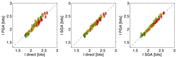
Figure 7 compares the three methods for computing the positional information carried by single gap genes in the
10–90% egg length segment. Across all four gap genes and all
four data sets the methods agree within the estimation error bars. This provides implicit evidence that, at least on the level of single genes, the Gaussian approximation holds
suf-ficiently well for our estimation methods.
Figure 6 Direct estimation for the positional information carried by Hunchback. (A) Extrapolation in sample size for different bin sizes D, starting with 10 bins for the bottom line and increasing to 50 bins for the top line in increments of 2. Black points are averages of naive esti-mates over 100 random choices ofmembryos (error bars = SD), plotted against 1/mon thex-axis. Lines and blue circles represent extrapolations to the infinite data limit, m/N. (B) The extrapolations to the infinite data limit (blue points from A) are plotted as a function of the bin size, and the second regression is performed (blue line) tofind the extrapola-tion ofD / 0. Thefinal estimate, represented by the red square, is
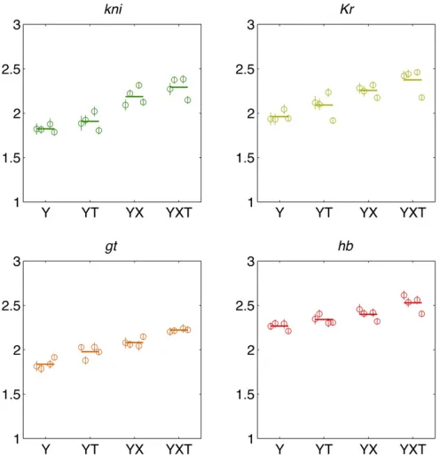
Figure 8 compares the estimation results across data sets and the alignment methods. With the exception of data set D data under T alignments, the information estimates are consistent across data sets. As expected, successive align-ment procedures remove systematic variability and increase the information by comparable amounts, so that the max-imal differences (between the minmax-imal Y alignment and the
maximal XYT alignment) are25%, 21%, 21%, and 11%
forkni,Kr,gt, andhb, respectively, when averaged across data sets.
Merging data from different experiments: To compute positional information carried by multiple genes from our data, using the second Gaussian approximation, we need
to measure Nmean profiles,giðxÞ;and theN3N
covari-ance matrix, Cij(x). While measuring giðxÞ is a standard
technique, estimating the covariance matrix, Cij(x),
requires the simultaneous labeling of all N gap genes in
each embryo, usingfluorescent probes of different colors.
While simultaneous immunostainings of two genes are not unusual, it is not easy to scale the method up to more genes while maintaining a quantitative readout. While for
data sets A–D we succeeded in doing a simultaneous
four-way stain, in general this is not alfour-ways feasible, so we developed an estimation technique for inferring a
consis-tent N 3 N covariance matrix based on multiple
collec-tions of pairwise stained embryos.
Estimating a joint covariance matrix from pairwise staining experiments is nontrivial for two reasons. First,
each diagonal element of the covariance matrix, i.e., the
variance of an individual gap gene, is measured in multiple experiments, but the obtained values might vary due to mea-surement errors. Second, true covariance matrices are posi-tive definite, i.e., det(C(x)) . 0, a property that is not
guaranteed by naivelyfilling in different terms of the matrix
by computing them across sets of embryos collected in
differ-ent experimdiffer-ents. This is a consequence of small sampling
errors that can strongly influence the determinant of the
ma-trix. We therefore need a principled way tofind a single best
and valid covariance matrix from multiple partial observa-tions, a problem that has considerable history in statistics
andfinance (see,e.g., Stein 1956; Newey and West 1986).
We start by considering a numberNijof embryos that have
been costained for the pair of gap genes (i,j). Let the full data set consist of all such pairwise stainings: for N gap genes, this is
a total of
N 2
pairwise experiments, where i,j= 1,. . .,N
and i , j. Thus, in the case of the four major gap genes in
Drosophila embryos, kni,Kr,gt, andhb, the total number of recorded embryos isN ¼Pði;jÞNij;where the sum is across all
six pairwise measurements: (1, 2), (1, 3), (1, 4), (2, 3), (2, 4), (3, 4). These pairwise measurements give us estimates of the mean profile^giðxÞand the 232 covariance matrices for each pair (i,j),C^ijðxÞ:
For four gap genes and six pairwise experiments, we will
get six 2 3 2 partial covariance matrices ^C; and 6 3 2
estimates of the mean profile^g:Our task is to find a single set of four mean profilesgiðxÞand a single 434 covariance
matrix Cij(x) thatfits all pairwise experiments best. In the
next paragraphs, we show how this can be computed for the
arbitrary case of Ngap genes.
To infer a single set of mean profilesgiðxÞ and a single
consistentN3Ncovariance matrixCij(x), we use
maximum-likelihood inference. We assume that at each positionxour
data are generated by a singleN-dimensional Gaussian
dis-tribution of Equation 4 with unknown mean values and an
unknown covariance matrix, which we wish tofind, but we
can observe only two of the mean values and a partial co-variance in each experiment; the other variables are inte-grated over in the likelihood.
Following this reasoning, the log likelihood of the data for pairwise staining (i,j) at positionxis
Figure 7 Comparing estimation methods for positional information carried by single gap genes. Shown are the estimates for four gap genes (color coded as in Figure 5), using four data sets (data sets A, B, C, and D) and four different alignment methods (Y, YT, XY, and XYT), for 64 total points per plot. Dashed line shows equality. Different alignment methods result in a spread of information val-ues for the same gap gene, as shown explicitly in Figure 8.
Lij¼
1
Nijlog
Z Y
k6¼i;j
dgk PðfgigjxÞ
¼ 1
Nij
lnY
Nij
m¼1
3
exp
2ð1=2Þ
Cjj
gðimÞ2gi
2
þCii
gðjmÞ2gj
2
22CijgðimÞgðjmÞ
CiiCjj2C2ij
2p ffiffiffiffiffiffiffiffiffiffiffiffiffiffiffiffiffiffiffiffiffiCiiCjj2C2ij
where the log-likelihood L as well as the mean profiles,
covariance elements, and the measurements all depend onx;
indexmenumerates all theNijembryos recorded in a pairwise
experiment (i,j).
Since all pairwise experiments are independent measure-ments, the total likelihoodLtotðxÞat a given positionxis the sum of the individual likelihoodsLtotðxÞ ¼Pði;jÞLijðxÞ:After some algebraic manipulation, the total log likelihood can be written in terms of the empirical estimates for the mean profiles ^gi and covariances C^ij of the separate pairwise
experiments:
LtotðxÞ ¼ 2
P
ði;jÞlnð2pÞ þln
CiiðxÞCjjðxÞ2C2ijðxÞ
þ CjjðxÞC^ijðxÞ22giðxÞ^giðxÞ þg
2 iðxÞ
CiiðxÞCjjðxÞ2C2ijðxÞ
þ CiiðxÞ^CjjðxÞ22gjðxÞ^gjðxÞ þg
2 jðxÞ
CiiðxÞCjjðxÞ2Cij2ðxÞ þ 2CijðxÞ
3^CijðxÞ2^giðxÞgjðxÞ2g^jðxÞgiðxÞ þgiðxÞgjðxÞ
CiiðxÞCjjðxÞ2C2ijðxÞ :
For each positionx, we search forgiðxÞandCij(x) that maximize LtotðxÞ:Before proceeding, however, we have to guarantee
that the search can take place only in the space of positive semidefinite matricesCij(x) (i.e., detC$0). We enforce this
constraint by spectrally decomposingCijand parameterizing
it in its eigensystem (Pinheiro and Bates 2007). To this end,
we writeC(x) =PDPT, whereDis a diagonal matrix
param-eterized with the variables a1,. . .,aN that determine the
diagonal elements inD;i.e.,Dii= exp(ai). The orthonormal
matrix P is decomposed as a product of the N(N 2 1)/2
rotation matrices in N dimensions: P¼QkN¼ðN121Þ=2RkðukÞ;
where Rk(uk) is a Euclidean rotation matrix for angle uk
acting in each pair of dimensions indexed by k.
In the spectral representation, the likelihood is a function ofNvaluesgi;Nparametersai, andN(N21)/2 anglesukat
each x. In the case of four gap genes, this is a total of 14
parameters that need to be computed by maximizingLtotðxÞ
at each location x.
There is no guarantee that there is a unique minimum for the log likelihood; moreover, there could exist sets of covariance matrices that all lead to essentially the same
value forLtotðxÞ;or, even more dangerously, the
maximum-likelihood solution could favor matrices with vanishing determinants, especially when estimating from a small num-ber of samples. To address these issues, we regularize the
problem by replacing D/D+lI, whereIis the identity
matrix andlis the regularization parameter. Larger values
of l will favor more “spherical” distributions, while small
values will allow distributions that can be very squeezed
in some directions. We thus maximize Ltotðx;lÞtofind the
best set of parameters given the value of the regularizer
(which is assumed to be the same for every x). To set l
we use cross-validation: the maximum-likelihoodfit is
per-formed for various choices of lnot over all available data
(embryos), but only over a trainingsubset. The remaining
embryos constitute atestsubset. Parameterfits for different
l obtained on the training data can be assessed and
com-pared by evaluating their likelihood over test data and
selecting the value oflthat maximizes the model likelihood
over the testing set.
To compute giðxÞ andCij(x), we initializegiðxÞ to the
mean profile across all pairwise experiments (i, j); we
initialize aito the mean of the log of the diagonal terms
^
Cii; and we initialize all rotation angles uk = 0. The
Nelder–Mead simplex method is used to maximize LtotðxÞ
(Lagarias et al. 1998). Finally, we compute C(x) fromai
anduk.
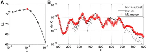
Finally, we use our quadruple-stained data sets to test our pairwise merging procedure. We partition the 102 embryos from data set D into six disjoint subsets of 14 embryos each (while retaining 18 embryos for validation), and in each subset we consider only one of the six possible pairs of gap gene data; that is, in every subset for a pair of genes (i,j), we measured the mean expression profilesgiðxÞ;gjðxÞ and
the 232 covariance matrixCij(x), the inputs to the
maximum-likelihood merging procedure. Note that this benchmark
uses real data from data set D, by simply “blacking out”
certain measured values so that for every embryo, only
one pair of gap genes remains visible to the merging
pro-cedure. The inferred 434 covariance matrix can be
com-pared to the covariance matrix estimated from the complete data set. The results of this procedure are shown in Figure 9, demonstrating that pairwise measurements can be merged into a consistent covariance matrix, whose determinant matches well with the determinant extracted from the com-plete data set. Note that determinants are compared because they are very sensitive to the inferred parameters and enter directly into the expressions for positional information and positional error. Importantly,filling in the covariance matrix naively, or skipping the regularization, results in either
non-positive-definite matrices or matrices whose determinants
are close to singular at multiple values of position x. The
presented maximum-likelihood merging procedure will al-low our framework to be applied to model systems where simultaneous gap gene measurements are hard to obtain, but pairwise stains are feasible.
Monte Carlo integration of mutual information: An-other technical challenge in applying the second Gaussian approximation for positional information to three or more gap genes lies in computing the entropy of the distribution of expression levels,S[Pg({gi})]. This is a Gaussian mixture
obtained by integrating P({gi}|x) over all xas prescribed
by Equation 27. In one or two dimensions one can evaluate this integral numerically in a straightforward fashion by
partitioning the integration domain into a grid with fine
spacing D in each dimension, evaluating the conditional
distributionP({gi}|x) on the grid for eachxand averaging
the results over x to get Pg({g}), from which the entropy
can be computed using Equation 9. Unfortunately, for three genes or more this is infeasible because of the curse of
dimensionality for any reasonablyfine-grained partition.
To address this problem we make use of the fact that over most of the integration domainPg({gi}) is very small
if the variability over the embryos is small. This means that most of the probability weight is concentrated in
the small volume around the path traced out inN
-dimen-sional space by the mean gene expression trajectory,giðxÞ;
as x changes from 0 to 1. We designed a method that
partitions the whole integration domain adaptively into volume elements such that the total probability weight
in every box is approximately the same, ensuring fine
partition in regions where the probability weight is con-centrated, while simultaneously using only a tractable number of partitions.
The following algorithm was used to compute the total entropy,S[Pg({gi})]:
1. The whole domain for {gi} is recursively divided into
boxes such that no box contains.1% of the total domain
volume.
2. For each boxiwith volumevi, we use Monte Carlo
sam-pling to randomly selectt= 1,. . .,Tpointsgtin the box
and approximate the weight of the box i as pðijxÞ ¼
viT21
PT
t¼1Pðg
tjxÞ; we explore different choices forTin
Figure 11.
3. Analogously, we evaluate the approximate total weight of
each box p(i), by pooling Monte Carlo sampled points
across allx.
4. p(i|x) andp(i) are renormalized to ensurePipðijxÞ ¼1
for everyxandPipðiÞ ¼1:
5. The conditional and total entropies are computed asSnoise¼ 2h
P
ipðijxÞlog2pðijxÞixand Stot ¼ 2
P
ipðiÞ
log2pðiÞ:
6. The positional information is estimated as I({gi}; x) =
Stot2Snoise.
7. The box i* = argmaxip(i) with the highest probability
weightp(i*) is split into two smaller boxes of equal
vol-umev(i*)/2, and the estimation procedure is repeated
by returning to step 2. Additional Monte Carlo sampling needs to be done only within the newly split box; for the other boxes old samples can be reused.
8. The algorithm terminates when the positional informa-tion achieves desired convergence or at a preset number of box partitions.
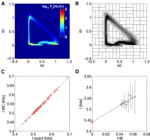
Figure 10, A and B, shows how the algorithm works for
a pair of genes ({hb,Kr}) for which the joint probability
distribution is easy to visualize. To get the final SGA
esti-mate of positional information that the two genes jointly
carry about position, extrapolation to infinite data size is
performed in Figure 10D.
Figure 11 shows the MC estimate of the positional in-formation carried by the quadruplet of gap genes and its
dependence on the parameterT(the number of MC
sam-ples per box per position) and the refinement of the
adap-tive partition. When T is too small (e.g., T = 100), we