Mathematical Modeling of Single Phase Flow and Particulate Flow Subjected to Microwave Heating

(1)

ABSTRACT

ZHU, JIANXI. Mathematical Modeling of Single Phase Flow and Particulate Flow Subjected to Microwave Heating. (Under the direction of Dr. Andrey V. Kuznetsov).

(2)

M

ATHEMATICAL

M

ODELING OF

S

INGLE

P

HASE

F

LOW AND

P

ARTICULATE

F

LOW

S

UBJECTED TO

M

ICROWAVE

H

EATING

By

J

IANXI

Z

HU

A dissertation submitted to the Graduate Faculty of North Carolina State University

in partial fulfillment of the requirements for the Degree of

Doctor of Philosophy

M

ECHANICAL

E

NGINEERING

Raleigh 2006

A

PPROVED

B

Y

:

___________________________ ___________________________

ANDREY V. KUZNETSOV K. P. SANDEEP

Chair of Advisory Committee

___________________________ ___________________________

(3)

BIOGRAPHY

(4)

ACKNOWLEDGEMENTS

My sincere gratitude should be first delivered to my advisor, Dr. Andrey V. Kuznetsov for his continuous support and guidance during my studies at NC State University. His enthusiasm in research and encouragement has been the driving force for the successful completion of my research and dissertation.

I gratefully acknowledge the support of this work by a USDA grant and Dr. K. P. Sandeep, for suggesting the project in the first place, and for critical advice and help for my research. My thanks would extend to Dr. William L. Roberts and Dr. Tarek Echekki for serving on my Ph.D. committee.

This major undertaking has received the generous support from my officemates, Ms. Ping Xiang. Her assistance, suggestions and encouragement are very important to me.

(5)

LIST OF TABLES

Table 2.1 Parameter values utilized in computations. ...31

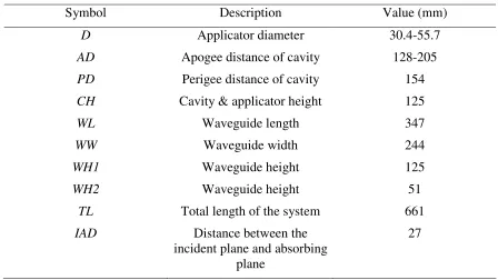
Table 3.1 Geometrical parameters. ...62

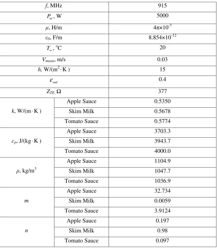
Table 3.2 Thermophysical and electromagnetic parameters utilized in computations...63

Table 3.3 Dimensionless power absorption in different liquids. ...64

Table 3.4 Dimensionless power absorption: effect of the applicator diameter...64

Table 3.5 Mean temperature increase at the outlet: effect of the applicator diameter...64

Table 3.6 Dimensionless power absorption: effect of the applicator location...65

Table 3.7 Dimensionless power absorption: effect of the cavity shape...65

Table 4.1 Geometric parameters...100

Table 4.2 Thermophysical and electromagnetic properties utilized in computations. ...100

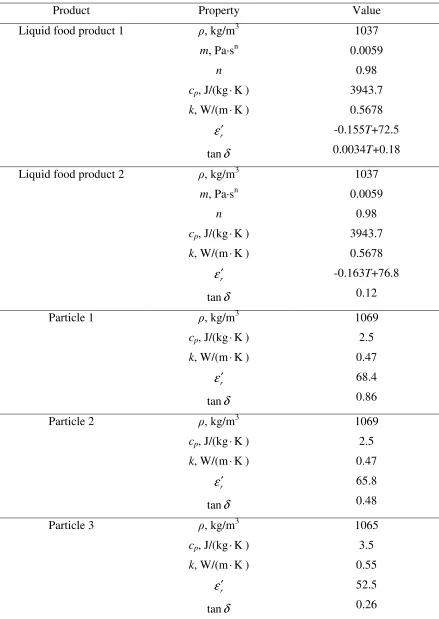
Table 4.3 Thermophysical and dielectric properties of food products. ...101

Table 5.1 Geometric parameters of the microwave system...140

Table 5.2 Comparison of the drag coefficient, CD, predicted by the code with published data [30]...140

Table 5.3 Thermophysical and electromagnetic properties utilized in computations. ...141

Table 5.4 Particles’ mean temperature at the applicator outlet, C...141

(11)

LIST OF FIGURES

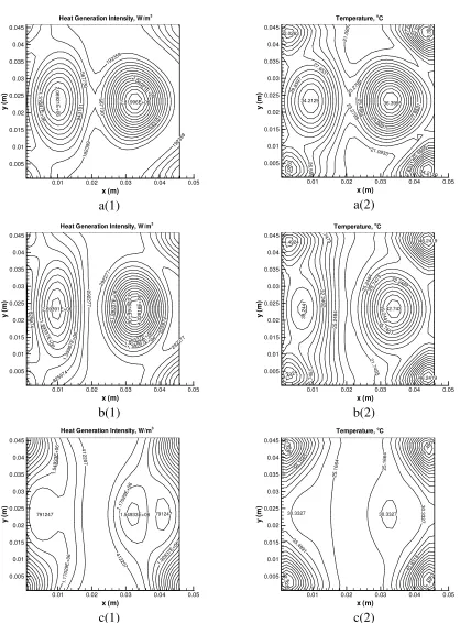
Figure 2.1 Schematic diagram of the microwave cavity and the applicator...32 Figure 2.2 Temperature dependence of the dielectric properties: (a) dielectric constant, ε′; (b) loss tangent, tanδ ...33 Figure 2.3 Electromagnetic heat generation intensity and temperature distributions at the outlet of the applicator: (a(1) – c(1)) electromagnetic heat generation intensity distributions (W/m3_{) for the apple sauce (a), skim milk (b), and tomato sauce (c),}

respectively; (a(2) – c(2)) temperature distributions (o_{C) for the apple sauce (a), skim}

milk (b), and tomato sauce (c), respectively. ...344 Figure 2.4 Standard deviation of the temperature distribution for the apple sauce, skim milk, and tomato sauce...35 Figure 2.5 Effect of the location of the applicator on heating the product: (a(1) – c(1)) electromagnetic heat generation intensity (W/m3) distributions at the outlet for the apple sauce (a), skim milk (b), and tomato sauce (c), respectively; (a(2) – c(2)) temperature (oC) distributions at the outlet for the apple sauce (a), skim milk (b), and tomato sauce (c), respectively, for the applicator having 141 mm off the original location in the x

direction. ...366 Figure 2.6 Effect of the size of the applicator on heating the product: (a(1) – c(1)) electromagnetic heat generation intensity (W/m3) distributions at the outlet for the apple sauce (a), skim milk (b), and tomato sauce (c), respectively; (a(2) – c(2)) temperature (oC) distributions at the outlet for the apple sauce (a), skim milk (b), and tomato sauce (c), respectively, for the applicator size of 60×60×124mm. ...377 Figure 3.1 Schematic diagram of the problem...66 Figure 3.2 Temperature dependent dielectric properties: (a) dielectric constant, ε′; (b) loss tangent, tanδ ...67 Figure 3.3 Temperature distributions (oC) in (a) x-z plane (y = 0), and (b) x-y plane (outlet, z

(12)

Figure 3.4 Electromagnetic power intensity distributions (W/m3) in (a) x-z plane (y = 0), and (b) x-y plane (outlet, z = 124mm) for apple sauce (1), skim milk (2), and tomato sauce

(3), respectively...69

Figure 3.5 Temperature distributions for tomato sauce at the outlet (z = 124mm): effect of the applicator position; the applicator is shifted in the x-direction from its position in the base case by (1) -136, (2) -68, (2) 0, (4) +68, (5) +136mm, respectively...70

Figure 3.6 Electromagnetic power intensity distributions for tomato sauce at the outlet (z = 124mm): effect of the applicator position; the applicator is shifted in the x-direction from its position in the base case by (1) -136, (2) -68, (2) 0, (4) +68, (5) +136mm, respectively. ...71

Figure 3.7 Temperature distributions for apple sauce at the outlet (z = 124mm): effect of the resonant cavity shape; (1) apogee distance of 205, (2) 186, (3) 167, (4) 154, and (5) 128mm, respectively. ...72

Figure 3.8 Electromagnetic power intensity distributions for apple sauce at the outlet (z = 124mm): effect of the resonant cavity shape; (1) apogee distance of 205, (2) 186, (3) 167, (4) 154, and (5) 128mm, respectively...73

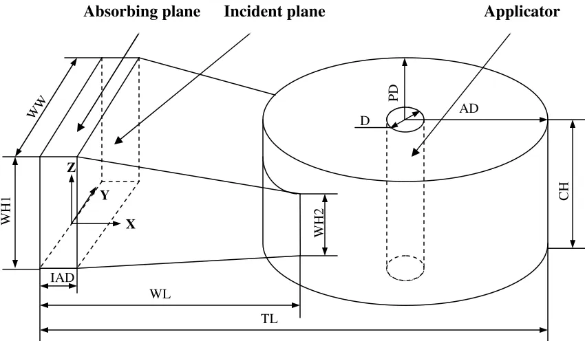
Figure 4.1 Schematic diagram of the microwave system. ...102

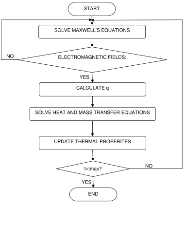
Figure 4.2 Computational algorithm...103

Figure 4.3 Basic arrangement for the particle inside the applicator. ...104

Figure 4.4 (a) Contour lines of the axial velocity of the fluid flow in the plane of symmetry of the applicator , and (b) streamlines in the plane of symmetry of the applicator: (1) before the particle entered the applicator; (2) t = 0.2 s ; (3) t = 0.65 s...105

Figure 4.5 (a) Trajectory of the particle in the plane of symmetry; (b) streamwise velocity of the particle...106

(13)

Figure 4.7 (a) Power density distributions (W/cm3) in the plane of symmetry of the particle, and (b) temperature distributions (oC) in the plane of symmetry of the particle for: (1) t

= 0.06 s; (2) t = 0.65 s; (3) t = 1.12 s....108 Figure 4.8 Surface temperature (oC) of the particle for: (a) t = 0.06 s; (b) t = 0.65 s; (c) t = 1.12 s....109 Figure 4.9 (a) Power density distributions (W/cm3) in the plane of symmetry of the particle, and (b) temperature distributions (oC) in the plane of symmetry of the particle at t = 1.4

s in: (1) particle 1; (2) particle 2; (3) particle 3...110 Figure 4.10 (a) Mean power density (W/cm3) in the particle; (b) mean power density in the liquid. ...111 Figure 4.11 Power density distribution (W/cm3) for: (a) liquid 1; (b) liquid 2. ...112 Figure 4.12 (a) Power density distributions (W/cm3) in the plane of symmetry of the particle, and (b) temperature distributions (o_C_{) in the plane of symmetry of the particle at}_t_{= 1.4}

s with: (1) carrier liquid 1; (2) carrier liquid 2...113 Figure 4.13 Power density distributions (W/cm3_{) in the plane of symmetry of the particle with}

different initial positions of the particle: (a) r=0.95cm and θ=0 ; (b) r=0.67cm

andθ=0 ; (c)r=0.28cm andθ =180 ; (d) r=0.67cm and θ =180 ; and (e) r=0.95cm and

180

θ= ...114 Figure 5.1 (a) Schematic diagram of the microwave system; (b) Basic arrangement for the particles inside the applicator...142 Figure 5.2 Schematic diagram for calculating contact forces of the inter-particle and

particle-wall collisions. ...143 Figure 5.3 Comparison of numerical and analytical solutions for field components. Solid line: numerical solution; circles: analytical solution...144 Figure 5.4 Contour lines of the axial velocity of the fluid flow in the planes corresponding to

0

(14)

Figure 5.6 Transient distributions: (a) microwave power density, W/cm3, (b) temperature, C

...147 Figure 5.7 Microwave power density and temperature distributions inside particles: (a) particle #15, (b) particle #19...148 Figure 5.8 (a) Particles’ mean temperature at the outlet of the applicator, C; (b) Mean power density in the mixture of the liquid and the particles, W/cm3. ...149 Figure 5.9 Power density distribution at the outlet of the applicator, W/cm3. ...150 Figure 5.10 Distribution of electric field component,Ez, (V/m): (a) base case; (b) +11.6 cm

(15)

1 INTRODUCTION

1.1 M

ICROWAVE

H

EATING

Microwave heating is utilized to process materials for decades. The ability of microwave radiation to penetrate the material directly without the need for any intermediate heat transfer medium provides a new and significantly different tool for processing a variety of industrial materials. When compared with conventional heating methods, where heat is conducted from surface into the interior volume of the specimen, microwave energy causes volumetric heat generation in the material, which results in high energy efficiency and a reduction in heating time. This is especially desirable for specimen of thick section and materials with low thermal conductivities, where surface heat may require much time to diffuse though the specimen.

(16)

mixture continues to absorb microwave energy until it fuses and vitrifies. In a similar process, infectious medical wastes can be irradiated prior to disposal, eliminating the need for incineration and off-sit treatment [3]. All these extensive applications of microwave heating stem from the great advantages of microwave heating over the traditional heating methods.

1.2 M

ICROWAVE

P

ROCESSING

D

EVICE

Microwaves are defined as electromagnetic waves with frequencies in the range from 300 MHz to 300 GHz. The corresponding wavelengths are from 10 cm to 0.1 cm. A microwave system typically consists of a generator to produce the microwaves, a waveguide to transport the microwaves and a cavity to manipulate microwaves for a specific purpose. Microwave cavities are classified as either single-mode, where a single standing electromagnetic wave fills the cavity, or multimode, where the cavity dimensions and microwave source frequency produce multiple standing waves. Single-mode cavities have had limited applications in industry because of a limited processing volume over which the electric field is useful, but have been particularly effective in plasma processing, joining and fiber curing. In a multimode system, the fixed frequency microwaves yield resonant modes over a narrow frequency band around the operating frequency. The modes result in regions of high and low electric fields within the cavity. In general, the uniformity of the field increases as the cavity size increase, but the uniformity also is dependent on the overall cavity dimensions [4].

(17)

frequency and phase. Gyrotrons offer the possibility of providing much higher power output (megawatts) and beam focusing. The traveling wave tubes can provide variable and controlled frequencies of microwave energy. Magnetrons are by far the most widely used microwave source for home microwave ovens and industrial microwave systems, due to their availability and low cost. Solid state devices also are available for generating microwaves, but typically have been limited in power (few tens of watts) [5].

(18)

material is strongly dependent on the internal electric field. In turn, the internal field is controlled by the field inside the cavity, which can vary widely in most cavities [5].

1.3 D

IELECTRIC

P

ROPERTIES OF

M

ATERIALS

Microwave radiation penetrates a material and produces a volumetrically distributed heat source, due to molecular friction resulting from dipolar rotation of polar solvents and fro the conductive migration of dissolved ions. The dipolar rotation is caused by variations of the electric and magnetic fields in the material [8]. Water, a major constituent of many materials is the main source of microwave interactions due to its dipolar nature [9]. When microwaves are applied to the material, forces on the charged particle from the oscillating electric field cause charged particles to move away from their equilibrium positions. This gives rise to induced dipoles which respond to the applied field. These dipoles are inclined to reoriented themselves in response to the changing electric field. The resistance to the reorientations of the dipole causes losses, attenuating the electric field and heating the material volumetrically. When a specimen is placed in a microwave cavity, the propagating microwave will penetrate and travel through the specimen. Once a steady root-mean-square electric field is achieved in the microwave cavity and specimen, the oscillating electric field within the material serves as a volumetric heat source. If the frequency of the electric field is near the natural frequency at which dipole reorientation occurs, the amount of heat generated within the material is maximized [2].

(19)

microwave propagation in a dielectric material are complex permittivity,

ε

, and the complex permeability,µ :

i

ε ε= −′ ε′′ (1.1)

i

µ µ= −′ µ′′ (1.2)

The real part of the complex permittivity,ε′ , is the relative permittivity, and the imaginary part,ε′′, is called the effective loss factor. The real part of the complex permeability,µ′, is referred to as the relative permeability, and the imaginary part,µ′′, is the magnetic loss factor.

The amount of microwave energy that the specimen absorbs depends strongly on the dielectric properties of the material. For insulating (non-magnetic) materials, the complex permittivity,

ε

, indicates the ability of the material to store and absorb energy from the oscillating electric source field. The relative permittivity,ε′ , indicates the penetration of microwave into the material. And the effective loss factor, ε′′ , characterizes the ability to store energy.

In addition, two alternative parameters, the loss tangent, , and the absorption coefficient, , are used to characterize the ability of the material to absorb microwave energy. They are defined as [10]:

tanδ ε ε ′′ =

′ (1.3)

0

2 f e

σ = π ε ε′′+σ (1.4)

where f is the microwave frequency, ε₀ is the permittivity of free space or vacuum, and

e

(20)

evident that the absorption of microwave energy is not only proportional to the effective permittivity but also the microwave frequency.

1.4 N

UMERICAL

M

ODELING OF

M

ICROWAVE

H

EATING

P

ROCESS

The intensity and spatial distribution of microwave energy throughout a material specimen is dictated by the complexity of electromagnetic waves scattering and reflecting in the microwave unit, as well as absorption of electromagnetic waves within the material [11]. Factors that influence microwave heating include dielectric properties, volume, and shape of the material, as well as design and geometric parameters of the microwave unit [12]. These factors make it difficult to precisely control the heating process in order to obtain the desired temperature distribution in the material. Due to complexity of the physical process, numerical modeling has been widely utilized to study microwave heating [13].

(21)

In the past, a number of studies [17-24] have been documented that dealt with numerical modeling of microwave heating process by solving Maxwell’s equations. The finite difference time domain (FDTD) method developed by Yee [25] has been used to provide a full description of electromagnetic scattering and absorption and gives detailed spatial and temporal information of wave propagation. Due to its versatility in handling complex shaped objects, a wide range of frequencies and stimuli, and a variety of materials, including those which exhibit frequency and temperature dependence, the FDTD method has received increased attention. A comparison of the FDTD method and other widely used methods for simulating microwave propagation and electromagnetic-material interactions are be found in refs. [26,27]. Solutions of Maxwell’s equations using the FDTD method for a number of simplified cases are reported in Webb et al. [28]. Three-dimensional simulations of microwave propagation and energy deposition are presented in Liu et al. [19], Zhao and Turner [29], and Zhang et al. [30].

(22)

Although most previous studies of microwave heating focused on conduction heat transfer in a specimen, a few recent papers investigated natural convection induced by microwave heating of liquids; mathematical models utilized in these papers included the momentum equation. Datta et al. [37] investigated natural convection in a liquid subjected to microwave heating. In their study, the microwave energy deposition was assumed to decay exponentially into the sample based on Lambert’s law, which is valid only for a high loss dielectric material and a sample of large size.

Ratanadecho et al. [38] were the first who investigated, numerically and experimentally, microwave heating of a liquid layer in a rectangular waveguide. The movement of liquid particles induced by microwave heating was taken into account. Coupled electromagnetic, hydrodynamic and thermal fields were simulated in two dimensions. The spatial variation of the electromagnetic field was obtained by solving Maxwell’s equations with the FDTD method. Their work demonstrated the effects of microwave power level and liquid electric conductivity on the degree of penetration and the rate of heat generation within the liquid layer. Furthermore, an algorithm for resolving the coupling of Maxwell’s, momentum, and energy equations was developed and validated by comparing with experimental results.

1.5 D

ISSERTATION

S

TRUCTURE

(23)

(24)

trajectories of particles. The effect of the time interval between consecutive injections of two groups of particles on power absorption in particles is studied. The influence of the position of the applicator pipe in the microwave cavity on the power absorption and temperature distribution inside the liquid and the particles is investigated as well.

R

EFERENCES

1. Venkateswaran, S., Merkle, C.L. (1991) Numerical modeling of waveguide heated microwave plasmas, Multidisciplinary Applications of Computational Fluid

Dynamics, ASME, 129: 1-12.

2. Smith, S.E. (2001): Numerical modeling of hybrid dielectric heating within a multi

mode microwave cavity, MS thesis, Indiana University-Purdue University at

Indianapolis, IN.

3. Lagos, L.E., Li, W., Ebadian, M.A. (1995) Heat transfer within a concrete slab with a finite microwave heating source, International Journal of Heat and Mass Transfer, 38(5): 887-897.

4. Clark, D.E., Folz, D.C., West, J.K. (2000) Processing materials with microwave energy, Journal of Materials Science and Engineering, A287: 153-158.

5. Clark, D.E., Sutton, W.H. (1996) Microwave processing of materials, Annual Review of Materials Science, 26: 299-331.

6. Saltiel, C. Fathi, Z., Sutton, W. (1995) Materials processing with microwave energy,

Mechanical Engineering, 117: 102-105.

7. Chamchong, M., Datta, A.K. (1999) Thawing of foods in a microwave oven: I. effect of power levels and power cycling, Journal of Microwave Power and Electromagnetic Energy, 34: 9-21.

8. Alton, W.J. (1998) Microwave pasteurization of liquids, Society of Manufacturing

(25)

9. Oliveira, M.E.C., Franca, A.S. (2002) Microwave heating of foodstuffs, Journal of Food Engineering, 53: 347-359.

10.Metaxas, A.C. Meredith, R.J. (1983) Industrial Microwave Heating, Peter Peregrinus Ltd., London.

11.Clemens, J., Saltiel, C. (1995) Numerical modeling of materials processing microwave furnaces, International Journal of Heat and Mass Transfer, 39: 1665-1675.

12.Anantheswaran, R.C., Liu, L. (1994) Effect of viscosity and salt concentration on microwave heating of model non-Newtonian liquid foods in a cylindrical container,

Journal of Microwave Power and Electromagnetic Energy, 29: 119-126.

13.Zhang, Q., Jackson, T.H., Ungan, A. (2000) Numerical modeling of microwave induced natural convection, International Journal of Heat and Mass Transfer, 43: 2141-2154.

14.Saltiel, C., Datta, A. (1997) Heat and mass transfer in microwave processing, Adv. Heat Transfer, 30: 1-94.

15.Franca, A.S., Haghighi, K. (1996) Adaptive finite element analysis of microwave driven convection, International Communications in Heat and Mass Transfer, 23: 177-186.

16.O’Brien, K.T., Mekkaoui, A.M. (1993) Numerical simulation of the thermal fields occurring in the treatment of malignant rumors by local hyperthermia, Journal of

Biomechanical Engineering, 115: 247-253.

17.Jia, X., Bialkowski, M. (1992) Simulation of microwave field and power distribution in a cavity by a three dimensional finite element method, Journal of Microwave

(26)

18.Deepak, Evans, J.W. (1993) Calculation of temperatures in microwave-heated two-dimensional ceramic bodies, Journal of American Ceramic Society, 76: 1915-1923. 19.Liu, F., Turner, I., Bialkowski, M. (1994) A finite-difference time-domain simulation

of power density distribution in a dielectric loaded microwave cavity, Journal of

Microwave Power and Electromagnetic Energy, 29: 138-147.

20.Iwabuchi, K., Kubota, T., Kashiwa, T., Tagashira, H. (1997) Analysis of electromagnetic fields using the finite-difference time-domain method in a microwave oven loaded with high-loss dielectric, Electronics and Communications in Japan, 78: 41-50.

21.Dibben, D.C., Metaxas, A.C. (1997) Frequency domain vs. time domain finite element methods for calculation of fields in multimode cavities, IEEE Transaction on Magnetics, 33: 1468-1471.

22.Dibben, D.C., Metaxas, A.C. (1994) Finite element time domain analysis of multimode applicators using edge elements, Journal of Microwave Power and Electromagnetic Energy, 29: 243-251.

23.Kriegsmann, G.A. (1997) Cavity effects in microwave heating of ceramics, Journal of Applied Mathematics, 57: 382-400.

24.Araneta, J.C., Brodwin, M.E., Kriegsmann, G.A. (1984) High-temperature microwave characterization of dielectric rods, IEEE Transactions on Microwave Theory and Techniques, 32: 1328-1335.

(27)

26.Miller, E.K. (1994) Time-domain modeling in electromagnetics, Journal of

Electromagnetic Waves and Applications, 8: 1125-1172.

27.Iskander, M.F. (1992) Computer modeling and numerical techniques for quantifying microwave interactions with materials, Microwave Processing of Materials II, 189: 149-171.

28.Webb, J.P., Maile, G.L., Ferrari, R.L. (1983) Finite element implementation of three dimensional electromagnetic problems, IEEE Proceedings,78: 196-200.

29.Zhao, H., Turner, I.W. (1996) An analysis of the finite-difference time-domain method for modeling the microwave heating of dielectric materials within a three-dimensional cavity system, Journal of Microwave Power and Electromagnetic Energy, 31: 199-214.

30.Zhang, H., Taub, A.K., Doona, I.A. (2001) Electromagnetics, heat transfer and thermokinetics in microwave sterilization, AIChE Journal, 47: 1957-1968.

31.Ayappa, K.G., Davis, H.T., Davis, E.A., Gordon, J. (1992) Two-dimensional finite element analysis of microwave heating, AIChE Journal, 38: 1577-1592.

32.Ayappa, K.G., Brandon, S., Derby, J.J., Davis, H.T., Davis, E.A. (1994) Microwave driven convection in a square cavity, AIChE Journal, 40: 1268-1272.

33.Ayappa, K.G., Sengupta, T. (2002) Microwave heating in multiphase systems: evaluation of series solutions, Journal of Engineering Mathematics, 44: 155-171. 34.Basak, T., Ayappa, K.G. (1997) Analysis of microwave thawing of slabs with

(28)

35.Ratanadecho, P., Aoki, K., Akahori, M. (2002) The characteristics of microwave melting of frozen packed beds using a rectangular waveguide, IEEE Trans. on

Microwave Theory and Techniques, 50: 1495-1502.

36.Ratanadecho, P., Aoki, K., Akahori, M. (2002) Influence of irradiation time, particle sizes, and initial moisture content during microwave drying of multi-layered capillary porous materials, Journal of Heat Transfer, 124: 151-161.

37.Datta, A., Prosetya, H., Hu, W. (1992) Mathematical modeling of batch heating of liquids in a microwave cavity, Journal of Microwave Power and Electromagnetic Energy, 27: 38-48.

38.Ratanadecho, P., Aoki, K., Akahori, M. (2002) A Numerical and experimental investigation of the modeling of microwave heating for liquid layers using a rectangular wave guide (effects of natural convection and dielectric properties),

Applied Mathematical Modeling, 26: 449-472.

39.Zhu, J., Kuznetsov, A.V., Sandeep, K.P. (2005) Numerical simulation of forced convection in a duct subjected to microwave heating, Heat and Mass Transfer,

http://dx.doi.org/10.1007/s00231-006-0105-y (online first).

40.Zhu, J., Kuznetsov, A.V., Sandeep, K.P. (2005) Mathematical modeling of continuous flow microwave heating of liquids (effects of dielectric properties and design parameters), International Journal of Thermal Sciences, In press.sdfs

(29)

(30)

2 NUMERICAL SIMULATION OF FORCED CONVECTION IN A

DUCT SUBJECTED TO MICROWAVE HEATING

A

BSTRACT

In this chapter, forced convection in a rectangular duct subjected to microwave heating is investigated. Three types of non-Newtonian fluids flowing through the duct are considered, specifically, apple sauce, skim milk, and tomato sauce. A finite difference time domain method is used to solve Maxwell’s equations simulating the electromagnetic field. The three-dimensional temperature field is determined by solving the coupled momentum, energy, and Maxwell’s equations. Numerical results show that the heating pattern strongly depends on the dielectric properties of the fluid in the duct and the geometry of the microwave heating system.

Nomenclature

A area, m2

Cp specific heat capacity, J/(kg K⋅ )

c phase velocity of the electromagnetic propagation wave, m/s

E electric field intensity, V/m

f frequency of the incident wave, Hz

h effective heat transfer coefficient, W/(m2⋅K)

H magnetic field intensity, A/m

(31)

k thermal conductivity, W/(m K⋅ )

m fluid consistency coefficient

n flow behavior index

Nt number of time steps

p pressure, Pa

q electromagnetic heat generation intensity, W/m3

Q volume flow rate, m3/s

T temperature, o_C

t time, s tanδ loss tangent

w velocity component in the z direction, m/s

W width of the cavity, m

ZTE wave impedance,

Greek symbols

apparent viscosity, Pa⋅s

electric permittivity, F/m

ε′ dielectric constant

(32)

g wave length in the cavity, m

magnetic permeability, H/m density, kg/m3

electric conductivity, S/m

Superscripts

instantaneous value

Subscripts

ambient condition

0 free space, air in input

x,y,z projection on a respective coordinate axis

2.1 I

NTRODUCTION

(33)

non-uniformly [1-3]. Several factors affect the magnitude and uniformity of absorption of electromagnetic energy. These include dielectric properties, ionic concentration, volume, and shape of a product [4]. The power and temperature distributions inside the product can be predicted by solving the coupled momentum, energy, and Maxwell’s equations. Due to a large number of factors that affect heating and the complexity of the equations involved, numerical modeling is the only viable approach for conducting realistic process simulations [5].

(34)

power dissipation in a liquid is predicted by employing an FDTD method and the transient temperature and flow patterns in the liquid are simulated using the “SIMPLER” algorithm [12]; the two modules are coupled by temperature dependent dielectric properties of the liquid. A similar algorithm is adopted in the present study.

This chapter reports a numerical prediction of forced convection heat transfer occurring in a rectangular applicator within a three-dimensional microwave cavity. Three types of liquid foods are considered in this chapter to investigate the effect of dielectric properties on heating by simulating the steady-state temperature distributions in various liquids.

2.2 G

EOMETRY OF THE

S

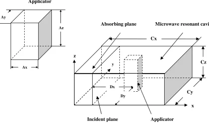
YSTEM

The microwave heating system, as illustrated in Figure 2.1, consists of a single mode microwave resonant cavity and a vertical applicator tube. The liquid flows through the applicator tube vertically upward, absorbing microwave energy during the process which heats the liquid.

As shown in Figure 1, the cavity dimensions (Cx × Cy × Cz) are 406 × 305 × 124mm. The applicator tube dimensions (Ax × Ay × Az) are 46 × 46 × 124mm. The applicator is located in the center of the cavity so that the centerline of the applicator is located at Dx = Cx/2 = 203mm and Dy = Cy/2 = 152.5mm. The microwave cavity is excited in TE10 mode [13] operating at a frequency of 915 MHz by imposing a plane

(35)

2.3 M

ATHEMATICAL

M

ODEL

F

ORMULATION

2.3.1 E

LECTROMAGNETIC

F

IELD

The equations governing the electromagnetic field are based on the Maxwell curl relation. The three-dimensional unsteady Maxwell’s equations in Cartesian coordinates are:

1 y

x E z

H E

t

µ

z y

∂

∂ ₌ ₋∂

∂ ∂ ∂ (2.1)

1

y z x

H E E

t

µ

x z

∂ ₌ ∂ ₋∂

∂ ∂ ∂ (2.2)

1 x y

z E E

H

t

µ

y x

∂ ∂

∂ ₌ ₋

∂ ∂ ∂ (2.3)

1 y

x z

x

H

E H _E

t

ε

y z

σ

∂

∂ ₌ ∂ ₋ ₋

∂ ∂ ∂ (2.4)

1

y x z

y

E H H

E

t

ε

z x

σ

∂ _∂ _∂

= − −

∂ ∂ ∂ (2.5)

1 y x

z

H H

E _E

t

ε

x y

σ

∂ ∂

∂ = − −

∂ ∂ ∂ (2.6)

where E and H are the electric and magnetic field intensities, is the electric conductivity, is the magnetic permeability, and is the electric permittivity.

The boundary conditions for the electromagnetic fields are:

(36)

0, 0

n t

H = E = (2.7)

At the absorbing plane, Mur’s [14] first order absorbing condition is utilized:

0 1

0 z x

E

z c t =

∂ ₋ ∂ ₌

∂ ∂ (2.8)

where c is the phase velocity of the propagation wave.

• At the incident plane, the input microwave source is simulated by the following equations:

, sin cos 2 in

Z inc in

g

x y

E E ft

W

π _π

λ

= − − (2.9)

, in sin cos 2 in

Y inc

TE g

E y x

H ft

Z W

π _π

λ

= − (2.10)

where Ein is the input value of the electric field intensity, Wis the width of the cavity, ZTE

is the wave impedance, and λg is the wave length of a microwave in the cavity.

2.3.2 H

EAT AND

M

ASS

T

RANSPORT

E

QUATIONS

The flow in the applicator is assumed to be hydrodynamically fully developed; only the streamwise velocity component is non-zero. The momentum equation is then presented as:

0

w w dp

x η x y η y dz

∂ ∂ ₊ ∂ ∂ ₋ ₌

∂ ∂ ∂ ∂ (2.11)

(37)

( 1)/ 2 2

2 n

w w

m

x y

η

−

∂ ∂

= +

∂ ∂ (2.12)

where m and n are the fluid consistency coefficient and the flow behavior index, respectively.

The temperature distribution in the liquid is obtained by solving the following energy equation wherein the microwave power absorption is accounted for by an electromagnetic heat source term:

2 2

p

T T T T

C w k q

t z x y

ρ

∂ + ∂ = ∂ +∂ +

∂ ∂ ∂ ∂ (2.13)

where q stands for the local electromagnetic heat generation intensity term, which is a function of dielectric properties of the liquid and the electric field intensity:

2 0

2 (tan )

q=

π ε ε

f ′

δ

E (2.14)

In Eq. (2.14),

ε

0is the permittivity of the air, ε′ is the dielectric constant of the liquid, and tanδ is the loss tangent, a dimensionless parameter defined as:

tan

δ

ε

′′ =

′ (2.15)

where ε′′ stands for the effective loss factor. The dielectric constant, ε′, characterizes the penetration of the microwave energy into the product, while the effective loss factor,

ε′′, indicates the ability of the product to convert the microwave energy into heat. Both

(38)

The following boundary conditions are utilized. At the inner surface of the applicator tube, a hydrodynamic no-slip boundary condition is used. At the inlet to the applicator, a uniform, fully developed velocity profile is imposed; it is specified by the inlet volume flow rate, Q. Heat transfer at the applicator wall is modeled as follows. The wall is assumed to lose heat by natural convection, which is modeled by the following equations:

at the walls normal to the x direction :

(

)

T

k h T T

x ∞

∂

− = −

∂ (2.16)

at the walls normal to the y direction :

(

)

T

k h T T

y ∞

∂

− = −

∂ (2.17)

where k is the thermal conductivity of the liquid and h is the effective heat transfer coefficient defined as:

1

1/ air wall/ wall 1/ liquid

h

h L k h

=

+ + (2.18)

(39)

T T= _∞ at t=0 (2.19)

2.4 C

OMPUTATIONAL

P

ROCEDURE

Two different time steps are utilized to update the electromagnetic and thermal-flow fields. An FDTD method [15] is used to solve Maxwell’s equations (2.1)-(2.6). The obtained electromagnetic fields are used to calculate the electromagnetic heat source, given by Eq. (2.14), which represents the heating effect of the microwave field on the liquid. Since in Eq. (2.14) the dielectric constant, ε′, and the loss tangent, tanδ , are temperature dependent, an iterative scheme is required to resolve the coupling of the energy and Maxwell’s equations. The time scale for electromagnetic transients (a nanosecond scale) is much smaller than that for the flow and thermal transport (a second scale). A time step in the block of the code that solves Maxwell’s equations must satisfy the stability requirement of the FDTD scheme [16] written as:

2 2 2

1 1 1

1

z y x c t

∆ + ∆ + ∆ ≤ ∆

(2.20)

The momentum and energy equations are solved by applying an implicit scheme; a time step of one second is utilized in these computations. The electromagnetic heat source, q, defined by Eq. (2.14), is computed in terms of the time average field, E , which is treated as a constant over one time step for the thermal-flow computation, and defined as:

1 1 Nt

t

E E

N τ

τ =

(40)

where Nt is the number of time steps in each period of the microwave and E

τ_{is the}

instantaneous E field. The details of the numerical scheme used in this chapter are given in ref. [17].

2.5 R

ESULTS AND

D

ISCUSSION

Table 2.1 shows electromagnetic and thermo-physical properties used in computations. The temperature-dependent data for the dielectric constant and loss tangent are plotted versus temperature in Figure 2.2.

2.5.1 H

EATING

P

ATTERNS FOR

L

IQUIDS WITH

D

IFFERENT

D

IELECTRIC

P

ROPERTIES

(41)

skim milk, while the intensities of the hot spots near the center of the tube are smaller. For the tomato sauce, from Figure 2.3-c(1-2), the peaks of the electromagnetic heat generation intensity disappear and there are no hot spots of the temperature in the central area of the applicator tube, only four hot spots at the corners. From this analysis it can be concluded that although the difference of dielectric properties of these three liquids is not great (see Figure 2.2), it causes a significant difference in their heating as they pass through the microwave cavity. In order to evaluate the uniformity of the temperature distribution quantitatively, a standard deviation of temperature is introduced as:

(

)

2

1

m

L T T dA

A

= − (2.22)

where A is the area of a cross-section perpendicular to the streamwise direction, and Tm is

(42)

(which is characterized by a medium loss tangent) and the apple sauce (which is characterized by the smallest loss tangent of the three products), which results in the peak value of the electromagnetic heat generation intensity; also, the temperature range (Tmax

-Tmin) for the tomato sauce is larger than that for the skim milk and the apple sauce. The

result is that the tomato sauce has the largest standard deviation of temperature at the outlet (the most nonuniform temperature distribution at the outlet) and the apple sauce has the most uniform temperature distribution.

2.5.2 E

FFECT OF

D

IFFERENT

L

OCATIONS OF THE

A

PPLICATOR ON THE

H

EATING

P

ROCESS

(43)

distributions of the electromagnetic heat generation intensity. This proves the significant effect of positioning the applicator tube in the microwave cavity on heating the product.

2.5.3 E

FFECT OF THE

S

IZE OF THE

A

PPLICATOR

The effect of the size of the applicator tube on heating patterns for the apple sauce is discussed in this paragraph. Figure 2.6 shows the electromagnetic heat generation intensity and temperature distributions of the three liquids at the outlet of the applicator with dimensions of 60×60×124mm. This applicator is larger than the applicator of the base size (46×46×124mm) although the enlarged applicator is positioned similarly in the center of the cavity, at the same location as the applicator of the base size. Comparing Figures 2.3 and 2.6, the distributions of the electromagnetic heat generation intensity and temperature are greatly affected by enlarging the applicator. For example, in the skim milk the peak value of the electromagnetic heat generation intensity and temperature in the applicator of a larger size are twice and three times larger than those in the applicator of the base size, respectively. This can be attributed to the fact that the larger applicator has a larger cross-sectional area allowing for more absorption of the microwave energy; also, for the same inlet volume flow rate, the flow in a larger applicator has a lower flow rate thus allowing fluid particles have larger residence time, which makes it possible for them to absorb more microwave energy.

2.6 C

ONCLUSIONS

(44)

(45)

Table 2.1 Parameter values utilized in computations.

Apple Sauce Skim Milk Tomato Sauce

f, MHz 915 915 915

E0, V/m 9000 9000 9000

, H/m 4 ×10-7 4 ×10-7 4 ×10-7

0, F/m 8.854×10-12 8.854×10-12 8.854×10-12

k, W/(m K⋅ ) 0.5350 0.5678 0.5774

cp, J/(kg K⋅ ) 3703.3 3943.7 4000.0

h, W/(m2⋅K) 30 30 30

, kg/m3 1104.9 1047.7 1036.9

Q, m3_/s _6.0×10-6 _6.0×10-6 _6.0×10-6

m 32.734 0.0059 3.9124

(46)

Figure 2.1 Schematic diagram of the microwave cavity and the applicator.

Applicator

x

y

z

Absorbing plane Microwave resonant cavity

Incident plane Applicator

Cy Cz Cx

Ax

Az

(47)

0 20 40 60 80 100 58

60 62 64 66 68 70 72 74 76

D

ie

le

ct

ri

c

co

ns

ta

nt

(

εεεε

/ )

Temperature (o_C)

Apple sauce Skim milk Tomato sauce

(a)

0 20 40 60 80 100

0.2 0.4 0.6 0.8 1.0 1.2 1.4

Lo

ss

ta

ng

en

t (

ta

n

δδδδ

)

Temperature (o_C)

Apple sauce Skim milk Tomato sauce

(b)

Figure 2.2 Temperature dependence of the dielectric properties: (a) dielectric constant,

(48)

1923 59 19235 9 1923 59 56 77 30 56 77 30 9431 01 9431 01 1.3 18 47_E +0₆ 2.0 692_1E +06 2.0 69 21 E +0 6 2.81996E+06 x (m) y (m )

0.01 0.02 0.03 0.04 0.05

0.005 0.01 0.015 0.02 0.025 0.03 0.035 0.04 0.045

Heat Generation Intensity, W/m3

a(1) 21.0933 21.0 933 23 .27 99 23.27 99 25_.4 66₅ 27.6 531 27.6 5 27.6 531 27.6 531 29.8 397 29.8₃₉₇ 32.0 26 34.2129 _36.3995 35.3 062 34.2129 32.0263 32.0 26 3 26 .5 59 8 25.46 65 x (m) y (m )

0.01 0.02 0.03 0.04 0.05

0.005 0.01 0.015 0.02 0.025 0.03 0.035 0.04 0.045 Temperature,o C a(2) 29 22 77 2922 77 2922 77 8259 74 82 59 74 8259 74 1.35 967E +06 1.35967E+ 06 1.8 93 37 E+

06 1.89337E

+06 4.0 28 16 E +0 6 2.69391E+06 4. 02 816E +0 6 1.89 337E +0 6 x (m) y (m )

0.01 0.02 0.03 0.04 0.05

0.005 0.01 0.015 0.02 0.025 0.03 0.035 0.04 0.045

b(1) 21_.7 49₅ 25 .2 484 25.2 484 8.7 47₃ 28.7 473 32 .2 46₂ 32.24₆₂ 35 .7 451 35.7₄₅₁ 39_.2 44₁ 39 .244 1 42.743 46.2419 44.4924 46.2419 44.4924 x (m) y (m )

0.01 0.02 0.03 0.04 0.05

0.005 0.01 0.015 0.02 0.025 0.03 0.035 0.04 0.045

Temperature,o_C

b(2) 41 22 07 1.928 37E+ 06

791247 1.54933E+06 791247

1.17 029E

+06 4122₀₇ 1.54 93 3E +0 6 1.17 029E +06 x (m) y (m )

0.01 0.02 0.03 0.04 0.05

0.005 0.01 0.015 0.02 0.025 0.03 0.035 0.04 0.045

c(1) 25 .1 66 4 35.4 991 45.8 318 56.1 645 92_.3 28₉ 97.4 953 97.4 953 92_.3 28₉ 30.3327 30.3327 30 .3 32 7 25.1 664 x (m) y (m )

0.01 0.02 0.03 0.04 0.05

0.005 0.01 0.015 0.02 0.025 0.03 0.035 0.04 0.045

Temperature,o_C

c(2)

(49)

0 20 40 60 80 100 120 140 0

5 10 15

20 Apple sauce_{Skim milk}

Tomato sauce

S

ta

nd

ar

d

D

ev

ia

tio

n

of

T

em

pe

ra

tu

re

(

0 C

)

z (mm)

(50)

45 51 23 4551 23 455 123 1.29₇₅₂ E+06 1.29 752E +06 2.13 991E

+06 2.9

8231E+ 06 5.5 09₄₉ E+ 06 1.29 752E +06 6.35189E+06 2.13991E+06 2.13 991E +06 2.13 991E +06 2.13991E+06 x (m) y (m )

0.01 0.02 0.03 0.04 0.05

0.005 0.01 0.015 0.02 0.025 0.03 0.035 0.04 0.045

a(1) 22.66₆₁ 27.99 83 33.3 304 33 .33₀₄ 33 .3 30 4 38_.66 26 38.6 626 38 .6 62₆ 54.6 591 27_.9 98₃ 38.6 626 59.9913 54.6 591 59 .99₁₃ 54_.6

59₁ 59.99₁₃

x (m)

y

(m

)

0.01 0.02 0.03 0.04 0.05

0.005 0.01 0.015 0.02 0.025 0.03 0.035 0.04 0.045

Temperature,o_C

a(2) 426767 1.2 25 4E +0₆ 1.22 54E+ 06 2.0 24₀₄ E+

06 2.82268E+064.41995E+06 6.01722E+06 1.62472E+06 1.62472E+06 5.2 18 59 E+ 06 4.819 27E+ 06 x (m) y (m )

0.01 0.02 0.03 0.04 0.05

0.005 0.01 0.015 0.02 0.025 0.03 0.035 0.04 0.045

b(1) 25 .98₄₉ 25.9 849 37.95 48 37.9 548 9.9 24₇ 49.92 47 73.86 45 67 .87₉₆ 10 9.7₇₄ 109.

774 49_.92

47 43.9398 x (m) y (m )

0.01 0.02 0.03 0.04 0.05

0.005 0.01 0.015 0.02 0.025 0.03 0.035 0.04 0.045

Temperature,o_C

b(2) 66 50 60 1.9 90 81_E +0₆ 3.97 945E +06 5.96 808E +06 5.9₆₈ 08 E+₀₆ x (m) y (m )

0.01 0.02 0.03 0.04 0.05

0.005 0.01 0.015 0.02 0.025 0.03 0.035 0.04 0.045

c(1) 28.6 165 63_.0 824 80.3₁₅₃ 97.5 483 149.247 149.247 45.84 94 x (m) y (m )

0.01 0.02 0.03 0.04 0.05

0.005 0.01 0.015 0.02 0.025 0.03 0.035 0.04 0.045

Temperature,o_C

c(2)

Figure 2.5 Effect of the location of the applicator on heating the product: (a(1) – c(1)) electromagnetic heat generation intensity (W/m3) distributions at the outlet for the apple

sauce (a), skim milk (b), and tomato sauce (c), respectively; (a(2) – c(2)) temperature (oC) distributions at the outlet for the apple sauce (a), skim milk (b), and tomato sauce

(51)

3809 68 380968 3809 68 1.13 067E +06 1.1 30 67_E +0₆ 1.13067E+06 1.13067E+06 5.6 28 91_E +0₆ 1.5₀₅₅ 3E +06 2.25 523E +06 1.8 80₃₈ E+ 06 x (m) y (m )

0.01 0.02 0.03 0.04 0.05 0.06 0.07 0.01 0.02 0.03 0.04 0.05 0.06

a(1) 24 .9 79 24.979 34 .9 37₁ 44.8952 64.8 113 64.8113 94.6856 64.8113 29 .9 58 1 94.6

856 44.8₉₅

2 54 .853 3 24.9₇₉ x (m) y (m )

0.01 0.02 0.03 0.04 0.05 0.06 0.07 0.01 0.02 0.03 0.04 0.05 0.06

Temperature,o_C

a(2) 303 386 903578 90 35 78 903578 1.50377E+06 2.10396E+06 3. 3043 4E+0 6 303386 6034 82 3.60 444E +06 6034 82 30 33₈₆ x (m) y (m )

0.01 0.02 0.03 0.04 0.05 0.06 0.07 0.01 0.02 0.03 0.04 0.05 0.06

b(1) 26.9961 26_.9 96₁ 40.9884 26.9 961 124.942 110. 95 54.98 07 40.9884 33.9 923 75.9₆₉ x (m) y (m )

0.01 0.02 0.03 0.04 0.05 0.06 0.07 0.01 0.02 0.03 0.04 0.05 0.06

Temperature,o_C

b(2) 5541 99 554199 2.186 73E+ 06 1.64 256E +06 2.7 309_1E +06 1.09838E+06 x (m) y (m )

0.01 0.02 0.03 0.04 0.05 0.06 0.07 0.01 0.02 0.03 0.04 0.05 0.06

c(1) 28_.6 50₈ 45.9₅₂₅ 80.555 9 80 .555 9 28.65 08 37.30 17 45.9 525 149. 763 14 9.7 63 89 .20 67 63_.2 54₂ 28 .65₀₈ x (m) y (m )

0.01 0.02 0.03 0.04 0.05 0.06 0.07 0.01 0.02 0.03 0.04 0.05 0.06

Temperature,o_C

c(2)

Figure 2.6 Effect of the size of the applicator on heating the product: (a(1) – c(1)) electromagnetic heat generation intensity (W/m3) distributions at the outlet for the apple

sauce (a), skim milk (b), and tomato sauce (c), respectively; (a(2) – c(2)) temperature (oC) distributions at the outlet for the apple sauce (a), skim milk (b), and tomato sauce

(52)

R

EFERENCES

1. Dibben, D.C., Metaxas, A.C. (1995) Time domain finite element analysis of multimode microwave applicators loaded with low and high loss materials,

Proceedings of the International Conference on Microwave and High Frequency

Heating,vol. 1-3, no. 4.

2. De Pourcq, M. (1985) Field and power density calculation in closed microwave system by three-dimensional finite difference, IEEE Proceedings,132 (11): 361-368. 3. Jia, X., Jolly, P. (1992) Simulation of microwave field and power distribution in a

cavity by a three dimensional finite element method, Journal of Microwave Power and Electromagnetic Energy,27(1): 11-22.

4. Anantheswaran, R.C., Liu, L. (1994) Effect of viscosity and salt concentration on microwave heating of model non-Newtonian liquid foods in a cylindrical container,

Journal of Microwave Power and Electromagnetic Energy, 29(2): 119-126.

5. Zhang, Q., Jackson, T.H., Ungan, A. (2000) Numerical modeling of microwave induced natural convection, International Journal of Heat and Mass Transfer, 43: 2141-2154.

6. Webb, J.P., Maile, G.L., Ferrari, R.L. (1983) Finite element implementation of three dimensional electromagnetic problems, IEEE Proceedings,78: 196-200.

7. Ayappa, K.G., Davis, H.T., Davis, E.A., Gordon, J. (1992) Two-dimensional finite element analysis of microwave heating, AIChE Journal, 38: 1577-1592.

8. Liu, F., Turner, I., Bialkowski, M. (1994) A finite-difference time-domain simulation of power density distribution in a dielectric loaded microwave cavity, Journal of

(53)

9. Zhao, H., Turner, I.W. (1996) An analysis of the finite-difference time-domain method for modeling the microwave heating of dielectric materials within a three-dimensional cavity system, Journal of Microwave Power and Electromagnetic Energy, 31(4): 199-214.

10.Zhang, H., Taub, A.K., Doona, I.A. (2001) Electromagnetics, heat transfer and thermokinetics in microwave sterilization, AIChE Journal, 47: 1957-1968.

11.Zhang, H., Datta, A.K. (2000) Coupled electromagnetic and thermal modeling of microwave oven heating of foods, Journal of Microwave Power and Electromagnetic Energy, 35(2): 71-85.

12.Patankar, S.V. (1980) Numerical heat transfer and fluid flow, Hemisphere, New York 13.Cheng, D.K. (1992) Field and wave electromagnetics, second ed., Addison-Wesley,

New York.

14.Mur, G. (1981) Absorbing boundary conditions for the finite difference approximation of the time domain electromagnetic field equations, IEEE Trans.

Electromag. Compat., EC-23: 377.

15.Yee, K.S. (1966) Numerical solution of initial boundary value problem involving Maxwell’s equations in isotropic media, IEEE Trans. On Antennas and Propagation, 14: 302-307.

16.Kunz, K.S., Luebbers, R. (1993) The finite difference time domain method for

electromagnetics, CRC, Boca Raton, FL.

(54)

3 MATHEMATICAL MODELING OF CONTINUOUS FLOW

MICROWAVE HEATING OF LIQUIDS (EFFECTS OF

DIELECTRIC PROPERTIES AND DESIGN PARAMETERS)

A

BSTRACT

In this chapter, a detailed numerical model is presented to study heat transfer in liquids as they flow continuously in a circular duct that is subjected to microwave heating. Three types of food liquids are investigated: apple sauce, skim milk, and tomato sauce. The transient Maxwell’s equations are solved by the Finite Difference Time Domain (FDTD) method to describe the electromagnetic field in the microwave cavity and the waveguide. The temperature field inside the applicator duct is determined by the solution of the momentum, energy, and Maxwell’s equations. Simulations aid in understanding the effects of dielectric properties of the fluid, the applicator diameter and its location, as well as the geometry of the microwave cavity on the heating process. Numerical results show that the heating pattern strongly depends on the dielectric properties of the fluid in the duct and the geometry of the microwave heating system.

Nomenclature

A area, m2

Cp specific heat capacity, J/(kg K⋅ )

c phase velocity of the electromagnetic propagation wave, m/s

E electric field intensity, V/m

(55)

h effective heat transfer coefficient, W/(m2⋅K)

H magnetic field intensity, A/m

L standard deviation of temperature, o_C

k thermal conductivity, W/(m K⋅ )

m _{fluid consistency coefficient,}_Pa_sn

n flow behavior index

N number of time steps

p pressure, Pa

q electromagnetic heat generation intensity, W/m3

Q microwave power absorption, W

T temperature, oC

t time, s

tanδ loss tangent

v fluid velocity vector, m/s

w velocity component in the z direction, m/s

W width of the incident plane, m

(56)

Greek symbols

apparent viscosity, Pa⋅s electric permittivity, F/m

ε′ dielectric constant

ε′′ effective loss factor

rad

ε

emissivity

g electromagnetic wavelength in the cavity, m

magnetic permeability, H/m density, kg/m3

electric conductivity, S/m

rad

σ

Stefan-Boltzmann constant, W/(m2 K4)

Superscripts

instantaneous value

Subscripts

(57)

in input

X,Y,Z projection on a respective coordinate axis

3.1 I

NTRODUCTION

Microwave heating is utilized to process materials for decades. In contrast to other conventional heating methods, microwave heating allows volumetric heating of materials. Without the need for any intermediate heat transfer medium, microwave radiation penetrates the material directly. Microwave energy causes volumetric heat generation in the material, which results in high energy efficiency and a reduction in heating time.

A distinct drawback to microwave heating is the lack of uniformity in material heating [1-3]. Both the magnitude and spatial distribution of microwave energy are dictated by the complexity of electromagnetic waves scattering and reflecting in the microwave unit, as well as absorption of electromagnetic waves within the material [4]. Factors that influence microwave heating include dielectric properties, volume, and shape of the material, as well as design and geometric parameters of the microwave unit [5]. These factors make it difficult to precisely control the heating process in order to obtain the desired temperature distribution in the material. Due to complexity of the physical process, numerical modeling has been widely utilized to study microwave heating [6].

(58)

determines the electromagnetic field in the microwave cavity and waveguide. The finite difference time domain (FDTD) method developed by Yee [15] has been widely utilized to solve Maxwell’s equations. Solutions of Maxwell’s equations using the FDTD method for a number of simplified cases are reported in Webb et al. [16]. Three-dimensional simulations of microwave propagation and energy deposition are presented in Liu et al. [9], Zhao and Turner [17], and Zhang et al. [18].

Success in the numerical simulation of electromagnetic propagation has recently generated interest in numerical modeling of heat transfer induced by microwave radiation. Clemens and Saltiel [4] developed a model of microwave heating of a solid specimen. Their model accounts for temperature dependent dielectric properties, which causes coupling between the Maxwell’s and energy equations. Effects of the microwave frequency, dielectric properties of the specimen, and the size of the sample on the microwave energy deposition were investigated in a two-dimensional formulation. Other important papers addressing modeling of microwave heating processes include Ayappa et al. [19-21], Basak et al. [22], and Ratannadecho et al. [23-24].

(59)

size samples or low loss dielectric materials, coupled Maxwell’s, momentum, and energy equations must be solved.

Ratanadecho et al. [26] were the first who investigated, numerically and experimentally, microwave heating of a liquid layer in a rectangular waveguide. The movement of liquid particles induced by microwave heating was taken into account. Coupled electromagnetic, hydrodynamic and thermal fields were simulated in two dimensions. The spatial variation of the electromagnetic field was obtained by solving Maxwell’s equations with the FDTD method. Their work demonstrated the effects of microwave power level and liquid electric conductivity on the degree of penetration and the rate of heat generation within the liquid layer. Furthermore, an algorithm for resolving the coupling of Maxwell’s, momentum, and energy equations was developed and validated by comparing with experimental results.

(60)

couple Maxwell’s and energy equations. In order to optimize the design of the microwave system, the effects of the diameter of the applicator tube, the location of the applicator tube in the microwave cavity, and the shape of the microwave cavity are investigated.

3.2 M

ODEL

G

EOMETRY

Figure 3.1 shows the schematic diagram of the microwave system examined in this research. The system consists of a waveguide, a resonant cavity, and a vertically positioned applicator tube that passes through the cavity. A liquid food, which is treated as a non-Newtonian fluid, flows through the applicator tube in the upward direction, absorbing the microwave energy as it passes through the tube. It is assumed that no phase change occurs during the heating process. The microwave operates in TE10 [30] mode at

Mathematical Modeling of Single Phase Flow and Particulate Flow Subjected to Microwave Heating

ABSTRACT

M

ATHEMATICAL

M

ODELING OF

S

INGLE

P

HASE

F

LOW AND

P

ARTICULATE

F

LOW

S

UBJECTED TO

M

ICROWAVE

H

EATING

J

Z

M

E

A

B

:

BIOGRAPHY

ACKNOWLEDGEMENTS

TABLE OF CONTENTS

LIST OF TABLES

LIST OF FIGURES

1

INTRODUCTION

1.1

M

H

1.2

M

P

D

1.3

D

P

M

ε

ε

1.4

N

M

M

H

P

1.5

D

S

R

2

NUMERICAL SIMULATION OF FORCED CONVECTION IN A

DUCT SUBJECTED TO MICROWAVE HEATING

A

2.1

I

2.2

G

S

2.3

M

M

F

2.3.1

E

F

µ

µ

µ

ε

σ