ABSTRACT
JI, XIANG. Phylogenetic Approaches for Quantifying Interlocus Gene Conversion. (Under the direction of Dr. Jeffrey L. Thorne and Dr. Sujit Ghosh).
This thesis presents various phylogenetic modeling strategies related to the
quantification of interlocus gene conversion (IGC) in multigene family evolution. IGC
mutations bring in additional correlation between paralog sequences by copying a sequence
stretch from the ‘donor’ paralog into the equivalent region of the ‘recipient’ paralog. The
results in this thesis indicate that the IGC rate can be substantial and should not be ignored.
The tools presented in this thesis can be applied to improve phylogeny inference, divergence
time estimation, and assorted other downstream analyses.
The first chapter reviews probabilistic models for sequence changes that arise via
point mutation. It also overviews background material concerning IGC mutations and
statistical methods for examining whether IGC has contributed to shaping observed genetic
variation.
The second chapter presents a composite likelihood strategy for incorporating IGC
into widely-used probabilistic models for sequence changes that originate with point
mutation. By applying this composite likelihood method, we estimated the percentage of
nucleotide substitutions that originate with an IGC event rather than a point mutation in 14
groups of yeast ribosomal protein-coding genes, and found values ranging from 20% to 38%.
In addition, we designed and applied a procedure to determine whether these percentages are
inflated due to artifacts arising from model misspecification. The results of this procedure are
The third chapter concentrates on how individual IGC events can simultaneously
affect a tract of consecutive sequence positions. We developed two new approaches for
estimating the tract lengths of sequence stretches that are fixed subsequent to an IGC
mutation. The first approach jointly considers two sites in a paralog as well as the
corresponding two sites in each other paralog. The second new IGC inference strategy adds a
hidden Markov model to our independent-site approach in order to estimate parameters
related to IGC tract length and IGC initiation rate.
The fourth chapter describes ongoing research directions. These include: strategies
for IGC inference in gene families that have large numbers of paralogs; the influence of IGC
on inferring the history of gene duplications; and how to incorporate asymmetry among
paralogs in IGC donor-recipient tendencies.
The fifth chapter discusses the scientific meaning of this work. We hope that IGC
tools presented in this thesis can be usefully applied and adapted so that a better
understanding of IGC in multigene evolution develops, and can offer the possibility of
© Copyright 2017 Xiang Ji
Phylogenetic Approaches for Quantifying Interlocus Gene Conversion
by Xiang Ji
A dissertation submitted to the Graduate Faculty of North Carolina State University
in partial fulfillment of the requirements for the degree of
Doctor of Philosophy
Bioinformatics and Statistics
Raleigh, North Carolina
2017
APPROVED BY:
_______________________________ _______________________________
Jeffrey L. Thorne Sujit Ghosh
Committee Co-Chair Committee Co-Chair
DEDICATION
BIOGRAPHY
Xiang Ji was born in Changchun, Jilin province China on August 22, 1988. His
childhood was similar to that of his role model scientist: “He attended school, grew up, and
attended school”1. Later, he moved to Beijing and attended school.
He earned his bachelor degrees in Physics and Economics (double major) from
Peking University, China in 2011. He then moved to North Carolina State University to
attend graduate school. He earned his master degree in Material Science and Engineering at
N.C. State in 2013. He switched to Bioinformatics (co-Major in Statistics) for his Ph.D.
degree so that he could work under Dr. Thorne’s direction. He will complete his Ph.D.
degree in 2017.
He learned to prepare for various possible outcomes at an early age from his parents.
His parents prepared him with the skill of playing the accordion so that he could at least enter
an art college and feed himself by teaching kids accordion. His parents prepared him with
math training starting at elementary school with the hope that it could help him with his
homework. His parents prepared him with English training, physics training, chemistry
training… His parents were not rich, but they were willing to spend half of their salary to pay
for his extra classes. Fortunately, most of his trainings paid off except for the writing courses.
1 Thorne, J. L. (1991). Pairwise sequence analysis: Evolutionary parameter estimation and
ACKNOWLEDGMENTS
I owe my career to two people: Dr. Liwen Zou and Dr. Jeffrey Thorne.
I deeply thank Dr. Alexander Griffing for his gracious help in every aspect.
I thank my committee members for bearing with and guiding me.
I thank everyone in Bioinformatics Research Center. The past four years has been enjoyable
TABLE OF CONTENTS
LIST OF TABLES ... viii
LIST OF FIGURES ... ix
Chapter 1 ... 1
1.1 Phylogenetic Trees ... 3
1.2 Continuous time Markov chains ... 5
1.3 Felsenstein’s pruning algorithm ... 6
1.4 Models of DNA Substitution ... 8
1.5 Models of Codon substitution ... 12
1.6 Homogeneity, Stationarity and Reversibility ... 13
1.7 Interlocus Gene Conversion ... 15
1.8 Existing Methods for Detecting IGC ... 17
1.8.1 Empirical Approach ... 18
1.8.2 Sawyer’s Method ... 19
1.8.3 The 4-2-4 Method ... 20
1.8.4 Innan’s Method ... 21
1.9 References ... 23
Chapter 2 ... 26
2.1 Abstract ... 26
2.2 Introduction ... 27
2.3 New Approaches ... 28
2.5 Discussion ... 40
2.6 Materials and Methods ... 43
2.7 Acknowledgments ... 47
2.8 References ... 50
Chapter 3 ... 53
3.1 Introduction ... 53
3.2 New approaches ... 54
3.2.1 Relaxation of the site-independent assumption ... 55
3.2.2 The PS approach ... 56
3.2.3 The HMM approach ... 60
3.3 Results ... 65
3.4 Materials and Methods ... 76
3.5 Discussion ... 77
3.6 Future Directions ... 81
3.7 References ... 82
Chapter 4 ... 84
4.1 Introduction ... 84
4.2 New approaches ... 84
4.2.1 IGC-Induced Gene Tree ... 86
4.2.2 Pairwise Marginal Likelihood (PML) Approach ... 88
4.2.3 A Data Augmentation Approach ... 91
4.4 Towards More Realistic IGC Models ... 102
4.4.1 Introduction ... 102
4.4.2 Directional IGC Rates Treatment ... 102
4.4.3 GC-biased IGC Rates Treatments ... 103
4.5 References ... 112
Chapter 5 ... 114
5.1 Inferring the evolution of multigene families ... 114
5.2 Whole genome duplication and gene tree incongruence ... 114
LIST OF TABLES
Table 2.1 Results of Analyzing 14 Paralogous Gene Pairs. ... 49
Table 3.1 HKY+IS-IGC results of Analyzing 14 Yeast Gene pairs. ... 68
Table 3.2 HKY+PS-IGC results of Analyzing 14 Yeast Gene pairs. ... 69
Table 4.1 Proportion of simulations with true tree topology T1 correctly inferred by the HKY+IS-IGC model p=0.05 ... 99
Table 4.2 Proportion of simulations with true tree topology T1 correctly inferred by the HKY+IS-IGC model p=0.005 ... 99
Table 4.3 Proportion of simulations that yielded inferences of either tree topology T2 or the true tree topology T1 correctly inferred by the HKY+IS-IGC model p=0.05 ... 99
Table 4.4 Proportion of simulations that yielded inferences of either tree topology T2 or the true tree topology T1 correctly inferred by the HKY+IS-IGC model p=0.005 ... 99
Table 4.5 Maximum Log-Likelihoods of Analyzing 14 Yeast Gene Pairs. ... 106
Table 4.6 Estimated τ values of Analyzing 14 Yeast Gene Pairs. ... 107
LIST OF FIGURES
Figure 1.1 A page from Darwin's notebook (Darwin 1837) ... 2
Figure 1.2 Species tree and Gene tree example. The species tree on the left shows the evolutionary relationship of four
species that are labeled with capital letters {A, B, C, D}. The gene tree on the right shows the evolutionary
relationship of seven genes from the four species. The multigene family comprising these seven genes arose via two
duplication events (the creation of red and blue lineages) and one gene loss event (the deletion in species D). The
genes are named by their species and a subscript number for each paralog. Genes with the same assigned number
coalesce (merge on the gene tree) by speciation events. Genes with different assigned numbers coalesce by
duplication events. ... 4
Figure 1.3 Interlocus gene conversion between and within chromosomes as in Chen et al. 2007 ... 15
Figure 1.4 Consequence of ignoring IGC. Left: what actually occurred. Right: what is inferred when IGC is ignored. The left
two panels show what actually occurred on a gene tree with three species and one duplication event that resulted in
two paralogs in each of the two ingroup species. There were one mutation event and one subsequent IGC event that
copied the mutation to the other paralog in both cases. The only difference between the two cases is the branch
where the two events happened. In the first case (top left panel), the two events happened on the post-speciation
branch that leads to one ingroup species. In the second case (bottom left panel), the two events happened on the
branch before the speciation event but after the duplication event. The right two panels in Figure 1.4 show what is
inferred under the parsimony criterion when IGC is ignored. For the first case, the sequence pattern would be
explained by two separate mutation events. For the second case, only one point mutation event would be preferred
to explain the sequence pattern and it is positioned on the wrong branch of the tree. The total number of events and
the distribution of root node state are affected in this case. ... 16
Figure 1.5 Scheme of Casola and Hahn simulation conditions. Each tip represents one paralog and the gene tree consists of
two rounds of duplication events. Two types of IGC events were simulated. The first type involved the two closest
paralogs (the left panel). The second type involved less closely related paralogs (the right panel). Arrows indicate
the direction of gene conversion as in Casola and Hahn (2009) ... 17
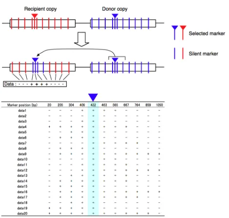
Figure 1.6 Illustration of a typical experiment to screen for gene conversion as in Mansai et al. 2011. The blue triangle
of the blue triangle, some function in the recipient copy could be induced and could be employed as a screen for IGC
events. For example, in yeast, if a gene for uracil or histidine is used, IGC could induce prototroph formation and this
could be a basis for selection. ... 18
Figure 1.7 Example segment of sequence pair in Sawyer’s method. ... 19
Figure 1.8 Pattern types considered by the 4-2-4 Method as in Ezawa et al. 2006. ... 21
Figure 2.1 The tree topology used for evolutionary analyses. The arrow indicates the branch on which the genome-wide
duplication occurred. ... 33
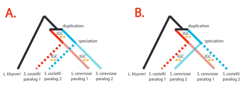
Figure 2.2 A paralog-swapping experiment addressing whether improvement to model fit can be attributed to IGC or to
artifacts. Both Scenarios A and B specify the correct rooted phylogeny between L. kluyveri and the paralogs of S.
castellii and S. cerevisiae. Scenario A shows the biologically correct situation that has IGC between paralogs in the
same genome. In Scenario B, IGC homogenization events involve one paralog from S. castellii and one from S.
cerevisiae. Because Scenario A corresponds to how observed data are generated, Scenario A should fit better than
Scenario B if IGC is actually being detected. Note that this paralog-swapping experiment would not be possible if only
1 post duplication species was used and would not be effective with more than two post duplication species. ... 35
Figure 2.3 Effect on parameter estimates of expected tract length. A. The mean estimate of τ among 100 simulated data
sets is plotted versus the expected length in nucleotides of IGC tracts. Vertical line segments depict interquartile
ranges of the estimates. The horizontal line shows the true value τ = 1.40948. B. The average among 100 simulated
data sets of the estimated proportion of nucleotide changes originating with IGC rather than point mutation is
plotted versus the expected length in nucleotides of IGC tracts. Vertical line segments depict interquartile ranges of
the estimates. The horizontal line at 0.2131 represents the estimate of the proportion of changes due to IGC in the
actual data. ... 37
Figure 2.4 Branch lengths from IGC and IND models for expected IGC tract length of 100 nucleotides. The Y-axis shows
average estimated values and interquartile ranges while the X-axis shows true values. All post-duplication branches
are depicted. The logarithmic scale on both axes as well as slight offsets of the IGC and IND model values are used to
enhance visibility. The dashed diagonal line shows where estimated values equal true values. ... 39
Figure 3.1 An HMM approach for inferring IGC tract lengths. A: The times of 5 IGC events are depicted on the branches of a
duplication, the lineage of one paralog is colored blue and the other is colored green. B: The times of the 5 IGC events
are depicted along the Y-axis and the paralog sequence regions affected by each IGC tract are shown in red on the
X-axis. At the bottom of the plot, sequence regions are colored red if they have experienced at least 1 IGC event on the
tree and are colored yellow otherwise. ... 60
Figure 3.2 The tree topology used for evolutionary analyses. The arrow indicates the branch on which the genome-wide
duplication occurred. ... 66
Figure 3.3 The gene tree topology of primate EDN ECP genes. The arrow indicates the duplication event. ... 70
Figure 3.4 MG94+IS-IGC+HMM result of EDN, ECP gene pair. A: log posterior probability ratio of hidden states and Viterbi
path along sites. B: log likelihood surface versus average tract length 1/p. ... 72
Figure 3.5 Effect on tract length parameter estimates from the pair-sites composite likelihood IGC procedure of expected
tract length. The mean of estimated tract lengths below 10-fold of expected tract length among 100 simulated data
sets is plotted versus the expected length in nucleotides of IGC tracts. Vertical line segments depict interquartile
ranges of the estimates. The dashed line depicts the Y=X line. ... 74
Figure 3.6 Effect on tract length parameter estimates from the HMM IGC procedure of expected tract length. The mean of
estimated tract lengths below 1000 nucleotides and 10-fold of expected tract length among 100 simulated data sets
is plotted versus the expected length in nucleotides of IGC tracts. Vertical line segments depict interquartile ranges of
the estimates where values higher than 1000 nucleotide are truncated to 1000 nucleotides. The dashed line depicts
the Y=X line. ... 75
Figure 4.1 Examples of IGC-induced gene trees. (A) Three IGC events are depicted with red showing the IGC tracts
associated with each event. These events combine to induce different histories for sites in different paralog regions.
The induced histories for paralog region I and II are illustrated. (B) A paralog tree showing two rounds of duplication
events followed by a speciation event create two species (A, B) with three paralogs in each species ({A1, A2, A3} and
{B1, B2, B3}). (C) The only IGC event that affects paralog region I (e.g., IGC1) is mapped onto the paralog tree. (D) The IGC-induced tree for paralog region I. (E) All 3 IGC events (IGC1, IGC2, IGC3) affect paralog region II and these are
mapped onto the paralog tree. (F) The IGC-induced tree for paralog region II. ... 87
Figure 4.2 Example of five paralog lineages embedded in one species tree branch of duration T. One IGC event happens at
time t1 and another happens at t2. Both IGC events will be assumed to affect the paralog region of interest. For
Figure 4.3 The gene family went through two rounds of tandem duplication before the speciation event that created the
two ingroup species. The branch lengths on the tree are defined by two parameters a and b. ... 94
Figure 4.4 The 10 gene tree topologies considered in the analyses. Topology 1 is the true tree topology under which the
simulated datasets were generated. The remaining 9 topologies represent all others that are possible subject to the
assumptions noted in the text. Based on the number of duplication events, the 10 gene tree topologies can be
grouped into 3 categories: {T1, T2}, {T3, T4, T5, T6}, {T7, T8, T9, T10}. ... 97
Figure 4.5 The Nesting Structure of the Five Models. Arrows point to the more general models that have one more degree
of freedom relative to the models where the arrows start. ... 109
Figure 5.1 Example of IGC-caused gene tree incongruence. (A) A gene tree of 3 extant genes (A2, B2, C1) embedded in their
species tree. After the whole genome duplication, one paralog with ‘x’ was lost in each species. Gene tree branches
with red show the gene tree topology between the three extant genes if there is no IGC event. (B) The gene tree
topology of the three extant genes if there is no IGC event. (C) An IGC event between paralog A1 and A2 affects the
gene tree topology of the three extant genes as indicated by the red arrow. (D) The gene tree topology of the three
Chapter 1
Introduction
Quests for origins never stop. Despite the philosophical nature of the quests, scientists have
been seeking the origins of our world and all life forms for centuries. With the cosmic
microwave background as its strongest support, now the origin of the universe is widely
accepted and explained by the Big Bang theory (Hawking et al. 1970; de Bernardis et al.
2000; Partridge 2007). There are several theories on how life started but none of them
dominate (Gilbert 1986; Segré 2001; Shapiro 2007;). Although the mechanism of how life
started is still in-debate, it is widely accepted that all living life forms are probably descended
from one common ancestral species, named as the last universal common ancestor (LUCA).
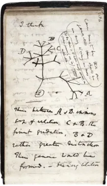
This idea was first proposed by Charles Darwin in his On the Origin of Species (Darwin 1859). Darwin’s work was based on morphological evidence. He suggested a tree structure to explain the evolutionary relationships among species (see Figure 1.1). Such a tree is also
Figure 1.1 A page from Darwin's notebook (Darwin 1837)
The emergence of molecular data provided a new data source for phylogeny
reconstruction. After the success of parsimony and distance-based methods, the field of
phylogenetics gradually adopted likelihood-based statistical approaches to infer unobserved
phylogenies from DNA and protein sequence data (Felsenstein 2004). With more and more
species being sequenced, the resolution of the species tree kept improving and its size
increased. The tree of life is no longer a mythical concept, but a practical collaborative
project among scientists across the world. As Yang and Rannala pointed out in their review
(Yang and Rannala 2012): “Today, phylogenies are used in almost every branch of biology.
Besides representing the relationships among species on the tree of life, phylogenies are used
to describe relationships between paralogues in a gene family, histories of populations, the
evolutionary and epidemiological dynamics of pathogens, the genealogical relationship of
somatic cells during differentiation and cancer development and the evolution of language.”
phylogenies can convey, phylogenies are also important from a statistical perspective
because they help to define the correlation structure that exists in biological data. In fact,
"tree-thinking" influences every biologist and is the reason why the famous Dobzhansky
(1973) quotation “Nothing in Biology Makes Sense Except in the Light of Evolution” is true.
In this chapter, I will briefly review the development of probabilistic models of
sequence evolution. These models are central to modern methods for phylogeny inference.
One deficiency of widely used models is that they tend to ignore a phenomenon known as
interlocus gene conversion (IGC). I will introduce this biological process and will also
overview existing methods for incorporating it into phylogenetic inference.
1.1 Phylogenetic Trees
It helps to distinguish between phylogenies that are gene trees and those that are species trees.
A species tree represents the evolutionary relationship of species. A gene tree represents the
evolutionary relationship among gene sequences. Often, there is no need to distinguish
between the two types of trees. One case where special attention is needed is multigene
family evolution. A multigene family is a set of homologous genes that originated from one
gene by duplication events as well as speciation events. Genes that are descended from a
common ancestral duplication are called paralogs. They usually have similar biochemical
functions but some may experience neo-functionalization where they acquire new functions
or sub-functionalization where the function of the original gene is divided and maintained
the loss of function. The new gene may lose its function by becoming a pseudogene (e.g. via
mutations that eliminate transcription or that introduce very early stop codons) or by being
removed from the genome due to a subsequent deletion.
Figure 1.2 Species tree and Gene tree example. The species tree on the left shows the evolutionary relationship of four species that are labeled with capital letters {A, B, C, D}. The gene tree on the right shows the evolutionary relationship of seven genes from the four species. The multigene family comprising these seven genes arose via two duplication events (the creation of red and blue lineages) and one gene loss event (the deletion in species D). The genes are named by their species and a subscript number for each paralog. Genes with the same assigned number coalesce (merge on the gene tree) by speciation events. Genes with different assigned numbers coalesce by duplication events.
Figure 1.2 shows an example of a species tree and a gene tree of a multigene family
that is embedded in that species tree. Usually, the evolutionary tree relating genes within a
multigene family is not directly observed. In such situations, there can be many alternative
duplication and deletion scenarios that can potentially explain a set of observed members of a
multigene family.
The gene tree in Figure 1.2 perfectly agrees with the species tree. Sometimes, the
lineage sorting, introgression, horizontal gene transfer, interlocus gene conversion, or other
sources. The possibility of such disagreement has inspired great research interest. The
problem of inferring species trees from known gene trees is reviewed by Szöllősi et al. 2014. A complementary inference problem is to infer a gene tree from a known species tree. This
inferential direction is also interesting, especially when people want to know the duplication
and loss history of a multigene family so that they can decipher how gene function has
changed over time.
1.2 Continuous time Markov chains
Continuous time Markov chains can describe the sequence changes on a phylogenetic tree
over the state space Φ. For example, the state space for nucleotides is Φ={A,C,G,T}.
Similarly, the state space for codons (or amino acids) is the set of codons (or amino acids).
Let the state of the chain at time t be X(t) which takes one of the values in Φ. The
substitution matrix (generator) Q={qij} characterizes the Markov chain. The off-diagonal
entry qij is the instantaneous rate of changes from state i to state j, that is,
qij = lim
Δt→0+Pr(X(t+Δt)= j|X(t)=i). And the diagonal entries of the substitution matrix are qii =− qij
j∈Φ,
∑
j≠i. Let p(t) be a vector specifying the probability distribution of the chain at
time t over the state space Φ. Therefore, p(t) has the same size as the state space Φ and has
its element pi(t)=Pr(X(t)=i). The vector p(t) is the solution to the following differential
dp(t)
dt = p(t)Q (4.1)
with the solution:
p(t)= p(0)eQt (4.2)
where p(0) is the probability distribution at the root node. The matrix exponentiation gives
the transition probability matrix M(t)=eQt. Note that the transition probability matrix is
usually denoted by P(t)in the literature, but is written as M(t) here to distinguish from the
probability distribution p(t) over states. The (i,j) entry in M(t) is the transition probability
from state i to state j after time t. In other words, the (i,j) entry in M(t) is
Pr(X(t)= j|X(0)=i). The stationary distribution of the Markov chain π must satisfy the following:
πQ=0 (4.3)
1.3 Felsenstein’s pruning algorithm
The pruning algorithm was first introduced by Dr. Joseph Felsenstein to calculate the
marginal probability of observing the sequence data at tips given the phylogenetic tree and
the substitution model (Felsenstein 1973). This likelihood marginalizes all possible sequence
states at the internal nodes of the phylogeny. The pruning algorithm was later recognized as a
special form of a dynamic programming algorithm. I will show the pruning algorithm using
the species tree in Figure 1.2. I use a bifurcating tree as an example just for convenience. A
branch splits, the result will always be exactly 2 new branches. The pruning algorithm can be
applied to any acyclic phylogenetic tree and multifurcation (i.e. splits of an old branch into 3
or more new branches) can be accommodated by the algorithm.
In Figure 1.2a, the species tree has a root node N1, 2 additional internal nodes
{N2,N3}, and 4 extant nodes {A,B,C,D}. The root of the tree represents the ancestral
lineage and the extant nodes represent current species. Therefore, time flows from the root
node to the leaves on the phylogenetic tree. For a time-reversible substitution model at
stationarity, the length of the branch connecting node N0 and N1 is unidentifiable. The
marginal likelihood of observing one column in the multiple sequence alignment of
{Xi ∈Φ,i=A,B,C,D} is:
L(θ)= f(XA,XB,XC,XD|θ)= f(X0,X1,X2,X3,XA,XB,XC,XD|θ) X3
∑
X2∑
X1∑
X0∑
(4.4)where θ is the set of parameter values in the model. By the Markovian property of the model, the state of the child node only depends on its parent node’s state and the length of the branch
that connects them. Therefore, the summation of joint likelihoods can be further broken
down into:
f(X0,X1,X2,X3,XA,XB,XC,XD|θ) X3
∑
X2∑
X1∑
X0∑
= f(XA,X2|X1,θ)f(XB,XC |X3,θ)f(XD,X3|X2,θ)f(X1|X0,θ)
X3
∑
f(X0|θ)X2
∑
X1∑
X0∑
= f(X0|θ) f(X1|X0,θ)
X1
∑
X0
∑
f(XA,X2|X1,θ)X2
∑
f(XD,X3|X2,θ)f(XB,XC|X3,θ)X3
∑
(4.5)
Let Li(Xi) denote the conditional likelihood of observing the data at or above the
node i has state Xi. For example, L3(X3)= f(XB,XC|X3,θ) and L2(X2)= f(XD,X3|X2,θ)f(XB,XC|X3,θ)
X3
∑
. Let p0 be the probability distribution of statesat the root node N0. The marginal likelihood can now be written as:
L(θ)= p0TL
0 (4.6)
and the conditional likelihood can be sequentially calculated (pruning) by:
Li= δXi if node i is a leaf node in state Xi
M(tl)Ll
(
)
!(
M(tr)Lr)
if node i has children l, r ⎧⎨ ⎪ ⎩⎪
(4.7)
where symbol ! denotes the pointwise product of two vectors which has the ith element
being
( )
u!v i=uivi, and where δXi denotes the vector with all zeros except for state Xi
having value 1.
1.4 Models of DNA Substitution
A wide variety of nucleotide substitution models have been employed for evolutionary
inference. As is usually the situation with likelihood-based inference, a compromise between
data set size and parameter-richness of a model must be made. However, likelihood-based
inference in the molecular evolution setting can also be computationally challenging and
sometimes the computational concerns motivate the choice of a probabilistic model of
sequence change. Rather than listing all nucleotide substitution models that have been
employed and we focus on some of those that have been used so often that the specific model
parameterizations have been named.
Jukes and Cantor (1969) proposed the first DNA substitution model. The JC69 model
assumes equal base frequency at stationarity and equal rates of all substitutions. The JC69
model has the form:
Q=
A C G T
A C G T . λ λ λ λ . λ λ λ λ . λ λ λ λ . ⎛ ⎝ ⎜ ⎜ ⎜ ⎜ ⎞ ⎠ ⎟ ⎟ ⎟ ⎟ (4.8)
where the diagonal entries are written “.” rather than specifying that the value of each
diagonal entry is the negative sum of the off-diagonal elements in that row.
The four nucleotides are often divided into two groups according to their chemical
properties. Specifically, Adenine and Guanine are purines and Cytosine and Thymine are
pyrimidines. Substitutions within the same chemical group are called transitions whereas
those between groups are called transversions. Typically, transitions happen more frequently
than transversions. Kimura (1980) incorporated a new parameter κ to represent the
transition/transversion rate ratio. The Kimura 2 parameter model (K2P) model has the form:
Q= . λ κλ λ λ . λ κλ κλ λ . λ λ κλ λ . ⎛ ⎝ ⎜ ⎜ ⎜ ⎜ ⎞ ⎠ ⎟ ⎟ ⎟ ⎟ (4.9)
Felsenstein (1981) incorporated nucleotide frequencies into the rate matrix. The F81
Q=
. πC πG πT πA . πG πT πA πC . πT πA πC πG . ⎛ ⎝ ⎜ ⎜ ⎜ ⎜ ⎜ ⎞ ⎠ ⎟ ⎟ ⎟ ⎟ ⎟ (4.10)
Hasegawa, Kishino and Yano (1985) combined the ideas of K2P and F81 to reflect
that substitution rates are influenced by both the transition/transversion ratio and unequal
base frequencies. The HKY85 model has the form:
Q=
. πC κπG πT
πA . πG κπT
κπA πC . πT
πA κπC πG .
⎛ ⎝ ⎜ ⎜ ⎜ ⎜ ⎜ ⎞ ⎠ ⎟ ⎟ ⎟ ⎟ ⎟ (4.11)
Tamura and Nei (1993) further distinguished between the two types of transitions (
A↔G,C↔T). The TN93 model has the form:
Q=
. πC κ1πG πT
πA . πG κ2πT
κ1πA πC . πT
πA κ2πC πG .
⎛ ⎝ ⎜ ⎜ ⎜ ⎜ ⎜ ⎞ ⎠ ⎟ ⎟ ⎟ ⎟ ⎟ (4.12)
It is easy to see that JC69, K2P, F81 and HKY85 models are special cases of TN93
eQt=
πA+
πAπY
πR
e2+πG
πR
e3 πC(1−e2) πG+πGπY
πR
e2− πG
πR
e3 πT(1−e2)
πA(1−e2) πC+
πCπR
πY
e2+πT
πY
e4 πG(1−e2) πT+πTπR
πY
e2− πT
πY
e4
πA+
πAπY
πR
e2− ππA
R
e3 πC(1−e2) πG+
πGπY
πR
e2+
πA
πR
e3 πT(1−e2)
πA(1−e2) πC+
πCπR
πY
e2− ππC
Y
e4 πG(1−e2) πT+
πTπR
πY
e2+
πC πY e4 ⎛ ⎝ ⎜ ⎜ ⎜ ⎜ ⎜ ⎜ ⎜ ⎜ ⎜ ⎜ ⎞ ⎠ ⎟ ⎟ ⎟ ⎟ ⎟ ⎟ ⎟ ⎟ ⎟ ⎟ (4.13)
where e2 =exp(−t), e3 =exp
[
−(πRκ1+πY)t]
, e4 =exp[
−(πYκ2+πR)t]
, πY =πT +πC, andπR =πA+πG.
The general time reversible model (GTR) is a generalization of the TN93 model
(Tavaré 1986). It specifies base frequency and distinguishes all types of nucleotide
substitutions. The GTR model has the form:
Q=
. aπC bπG cπT
aπA . dπG eπT bπA dπC . πT cπA eaπC πG . ⎛ ⎝ ⎜ ⎜ ⎜ ⎜ ⎜ ⎞ ⎠ ⎟ ⎟ ⎟ ⎟ ⎟ (4.14)
For a single site, the most general DNA substitution model has 12 free parameters for
each substitution (Yang 1994). Let UNREST denote this model as implemented in baseml
(Yang 2007). The UNREST model differs from the GTR model by relaxing the
time-reversible property of the Markov process. The GTR and UNREST models do not have
closed form analytical solutions for the transition probability matrix. The UNREST model
Q=
. a b c
d . e f
g h . i
j k l .
⎛ ⎝ ⎜ ⎜ ⎜ ⎜ ⎞ ⎠ ⎟ ⎟ ⎟ ⎟ (4.15)
1.5 Models of Codon substitution
Codon substitution models were introduced by Schöniger et al. 1990. The most influential
codon substitution models were proposed by Muse and Gaut (1994) and Goldman and Yang
(1994). In these models, the codon triplet (consisting of three consecutive nucleotides that
specify an amino acid) is considered the unit of evolution. Stop codons are ignored in these
models. For the standard genetic code, this reduces the state space of codon-based model
from a size of 64 to the 61 non-stop codons. Because the 61 codons each represent exactly
one of 20 amino acids, the standard genetic code is degenerate. Codons that code for the
same amino acid are referred to as being synonymous. Nonsynonymous codons encode
different amino acids. The main improvement of codon substitution models is the
introduction of the nonsynonymous/synonymous ratio (usually denoted by ω), which is a
simple way to characterize natural selection at the protein level. The value of ω can be
categorized into three groups. When ω = 1, synonymous and nonsynonymous changes fix at
the same rate, representing neutral protein evolution. When ω < 1, nonsynonymous changes
are removed more often than synonymous changes, representing purifying selection. When ω > 1, nonsynonymous changes are more likely to fix, representing diversifying positive
Yang and Nielsen (1998) and Nielsen and Yang (1998) simplified the original model
of Goldman and Yang (1994) and incorporated three features of sequence evolution: the
transition/transversion rate ratio κ, the nonsynonymous/synonymous rate ratio ω, and
different codon frequencies (πJ for codon J). The instantaneous rate of the substitution from
codon I to codon J is specified as:
qIJ =
0 if I and J differ at two or three codon positions
πJ if I and J differ by a synonymous transversion κπJ if I and J differ by a synonymous transition ωπJ if I and J differ by a nonsynonymous transversion κωπJ if I and J differ by a nonsynonymous transition ⎧ ⎨ ⎪ ⎪ ⎪ ⎩ ⎪ ⎪ ⎪ (4.16)
The Muse and Gaut (1994) model differs from the above model by replacing the
codon frequency πJ with the nucleotide frequency πh when codon I and codon J differ at
exactly one position with type h∈{A,C,G,T} in codon J. The MG94 model has the
instantaneous rate of substitution from codon I to codon J being:
qIJ =
0 if I and J differ at two or three codon positions
πh if I and J differ by a synonymous difference ωπh if I and J differ by a nonsynonymous difference ⎧
⎨ ⎪
⎩
⎪ (4.17)
1.6 Homogeneity, Stationarity and Reversibility
A Markov chain is time-homogeneous if the elements in the rate matrix Q are independent of
example, p(0)=π such that πQ=0, then the Markov chain will be at equilibrium at all
times; such a chain is considered to be at stationarity.
A Markov chain is time reversible if it satisfies πiQij =πjQji, for all i≠ j. Except for
the UNREST model, the nucleotide substitution and codon substitution models described
above are time reversible. The reversibility property means that the Markov process will look
the same no matter in which direction time flows. When time reversibility and stationarity
are both assumed, likelihoods of phylogenies are identical for all possible placements of the
root node. In other words, the root of a tree is statistically unidentifiable for a time reversible
model at stationarity.
Stationarity is usually assumed in a phylogenetic model because it reduces the
number of parameters to estimate. If the model is true, the Markov process is likely to be
approximately at stationarity given the long evolutionary time from the last universal
common ancestor. The stationarity assumption is violated by certain biological processes.
For example, a horizontal transferred gene may not be at stationarity right after being
introduced into the new organism. Also, different regions of the genome may experience
different biological constraints and this can yield variation of evolutionary processes among
sequence positions. Similarly, mutation rate may differ among genomic locations. The
structure of the gene may pose additional constraint on its evolutionary process. Therefore,
the parameter estimates from one region in the genome may not be directly applicable to
1.7 Interlocus Gene Conversion
Interlocus gene conversion (IGC) homogenizes paralogs in a multigene family. It is
sometimes also referred to as non-allelic gene conversion. IGC involves overwriting a
stretch of DNA sequence in a recipient paralog with the corresponding DNA sequence from
the donor paralog. IGC events are initiated by a DNA double-strand break (DSB) in the
DNA of what will be the IGC recipient gene. IGC events are products of a DNA repair
mechanism that use intact homologous sequence as template. The recipient sequence and the
donor sequence can be on the same chromosome, or different chromosomes as shown in
Figure 1.3. The repair mechanism generally forms Holliday junctions and requires high
degrees of similarity between the two sequences. There are several mechanisms associated
with the formation of Holliday junctions (reviewed in Chen et al. 2007). With all of these
mechanisms, the result is that all or part of the sequence of the gene that has the initial DSB
is replaced by the sequence of the corresponding region from another gene in the same
multigene family.
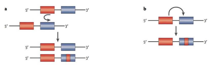
The copy-paste nature of the IGC process means that evidence of nucleotide
substitution in one paralog can be erased when IGC overwrites the sequence that experienced
it. In addition, IGC can make it appear as if parallel nucleotide substitutions independently
arose by point mutation in two different paralogs. Figure 1.4 shows two artificial examples of
how inference would be affected when IGC is ignored. Failure to consider IGC can obscure
the process of nucleotide substitution and potentially impact inferences of phylogenies.
Casola and Hahn (2009) showed that ignoring IGC would result in moderate false
detection of diversifying positive selection through simple simulation studies that combined
IGC with codon-based substitutions that originated via point mutation. They simulated
sequence data for three paralogs as shown in Figure 1.5. Casola and Hahn concluded that
branch length and gene conversion tract length both affect the false discovery rate of
diversifying positive selection.
Figure 1.5 Scheme of Casola and Hahn simulation conditions. Each tip represents one paralog and the gene tree consists of two rounds of duplication events. Two types of IGC events were simulated. The first type involved the two closest paralogs (the left panel). The second type involved less closely related paralogs (the right panel). Arrows indicate the direction of gene conversion as in Casola and Hahn (2009)
1.8 Existing Methods for Detecting IGC
This section will first summarize the empirical approach for detecting IGC and then will
1.8.1 Empirical Approach
As reviewed in Mansai et al. 2011, the empirical study of IGC involves transgenic
systems where a pair of genes are set up by transferring artificially edited DNA sequences
onto the same chromosome as shown in Figure 1.6. By examining the converted markers
around a selectable marker, an upper bound and a lower bound of the gene conversion tract
length can be estimated empirically. A caveat associated with this sort of empirical study is
the possibility that the details of the artificially engineered system may affect the generality
of the inferences. Also, this kind of scheme can only be used to study IGC in a relatively
small number of model genetic organisms.
1.8.2 Sawyer’s Method
Sawyer’s method is implemented in his widely used software GENECONV (Sawyer 1989).
It aims to evaluate the null hypothesis of no IGC. GENECONV analyzes a multiple
sequence alignment in a pairwise manner, searching for regions of sequence pairs that are
unusually similar relative to other regions of each sequence pair. The program first excludes
all invariant columns of the multiple sequence alignment and then looks for the highest
scoring segments of each induced pairwise alignment. The scoring system is designed to find
regions of high sequence identity by assigning positive scores to matches and negative scores
to mismatches. Figure 1.7 shows a high-scoring region for the sequence pair consisting of
Sequence #2 and Sequence #4.
Figure 1.7 Example segment of sequence pair in Sawyer’s method.
The program has two ways of calculating p-values. The first way is
based and the other is by a method of Karlin and Altshul (1990, 1993). The
permutation-based p-value is more accurate but takes more computational time. The columns of the
original multiple sequence alignment are shuffled to create a permuted alignment. The same
procedure of finding the highest scoring region for each sequence pair is applied to each
the proportion of permuted alignments for which the maximal score for that pair of sequences
is greater than or equal to the score for that pair of the highest-scoring region of the actual
(unpermuted) sequences. The "global permutation p-value" for a sequence pair of interest is
an attempt to design a conservative test for evaluating the null hypothesis of no IGC. It is
calculated by finding the highest scoring region for each sequence pair in each permuted
alignment and then taking the highest over all pairs of these high scores. The "global
permutation p-value" for the sequence pair of interest is the proportion of permuted
alignments for which the highest score over all sequence pairs is greater than or equal to the
highest scoring region of the actual sequences for the sequence pair of interest. Mansai and
Innan (2010) showed by simulation study that GENECONV could have limited power for
detecting IGC when the IGC rate is high.
GENECONV looks at sequence pairs to find sequence regions with high
conservation. It only searches for IGC evidence but it does not try to recover exact IGC
tracts. If a region only experienced one IGC event, GENECONV is likely to detect only a
subset of it as an IGC candidate. When a region experienced multiple IGC events, the
situation is more complicated. GENECONV may pick up a region that is longer than each
single IGC tract or several smaller subsets and this depends on how IGC events interact with
each other and on the amount of accumulated sequence variation.
1.8.3 The 4-2-4 Method
Ezawa et al. 2006 developed a quartet-based method that incorporates phylogenetic
Ezawa et al. 2006 approach as the 4-2-4 method. The 4-2-4 method uses two paralogous
genes (denoted by numbers 1 and 2 in Figure 1.8) from two species (denoted by M and R in
Figure 1.8) that are result of one gene duplication event and a subsequent speciation event. If
no gene conversion happened between the paralogs, the orthologous genes across species are
expected to be more closely related and therefore favor a (M1, R1) – (M2, R2) pattern as
shown with the type 1 pattern of Figure 1.8. If gene conversion homogenized paralogous
sequences, the type 2 pattern of (M1, M2) – (R1, R2) is more likely. The test searches for
longest type 2 tracts in the data as evidence of gene conversion. The test has a similar idea to
Sawyer’s approach but pays more attention to the extra information (or constraints) from the
phylogeny.
Figure 1.8 Pattern types considered by the 4-2-4 Method as in Ezawa et al. 2006.
1.8.4 Innan’s Method
Innan (Innan 2002, Innan 2003) developed a population genetics method for inferring IGC
the four haplotypes, A-A, A-a, a-A and a-a. Let x1, x2, x3, x4 denote the frequencies of the
four haplotypes wherex1+x2+x3+x4 =1. Let µ be the point mutation rate between the two
alleles, r be the recombination rate between two loci per generation, and c be the IGC rate
between the two loci. Then the gene frequency of next generation can be written as:
x1' =(1−2µ)x1+(µ +c)(x2+x3)−rD (4.18)
x2' =(1−2µ−2c)x2+µ(x1+x4)+rD (4.19)
x3' =(1−2µ−2c)x3+µ(x1+x4)+rD (4.20)
x4' =(1−2µ)x4+(µ +c)(x2+x3)−rD (4.21)
where D=x1x4−x2x3. By using the diffusion approximation (see Kimura 1964) and
assuming equilibrium, the frequencies and the expectations of the amounts of variation
(heterozygosity) within the two loci can be written as functions of the model parameters plus
the population size (see Innan 2002 for details). The parameters of the model can be
1.9 References
Casola, C., & Hahn, M. W. (2009). Gene conversion among paralogs results in moderate false detection of positive selection using likelihood methods. Journal of molecular evolution, 68(6), 679-687.
Chen, J. M., Cooper, D. N., Chuzhanova, N., Férec, C., & Patrinos, G. P. (2007). Gene conversion: mechanisms, evolution and human disease. Nature Reviews Genetics, 8(10), 762-775.
Darwin C. (1837) First diagram of an evolutionary tree from his First Notebook on Transmutation of Species.
Darwin C. (1859). On the origin of species. Cambridge University Press.
de Bernardis, P., Ade, P. A. R., Bock, J. J., Bond, J. R., Borrill, J., Boscaleri, A., ... & Ferreira, P. G. (2000). A flat Universe from high-resolution maps of the cosmic microwave background radiation. Nature, 404(6781), 955-959.
Dobzhansky, T. (1973). Nothing in biology makes sense except in the light of evolution. The american biology teacher, 35(3), 125-129.
Ezawa, K., OOta, S., & Saitou, N. (2006). Genome-wide search of gene conversions in duplicated genes of mouse and rat. Molecular biology and evolution, 23(5), 927-940.
Ezawa, K., Ikeo, K., Gojobori, T., & Saitou, N. (2010). Evolutionary pattern of gene homogenization between primate-specific paralogs after human and macaque speciation using the 4-2-4 method. Molecular biology and evolution, 27(9), 2152-2171.
Felsenstein, J. (1973). Maximum likelihood and minimum-steps methods for estimating evolutionary trees from data on discrete characters. Systematic Biology, 22(3), 240-249. Felsenstein, J. (1981). Evolutionary trees from DNA sequences: a maximum likelihood approach. Journal of molecular evolution, 17(6), 368-376.
Felsenstein, J. (2004). Inferring phylogenies (Vol. 2). Sunderland, MA: Sinauer associates.
Gilbert, W. (1986). Origin of life: The RNA world. Nature, 319(6055).
Hasegawa, M., Kishino, H., & Yano, T. A. (1985). Dating of the human-ape splitting by a molecular clock of mitochondrial DNA. Journal of molecular evolution, 22(2), 160-174. Hawking, Stephen W., and Roger Penrose. "The singularities of gravitational collapse and cosmology." Proceedings of the Royal Society of London A: Mathematical, Physical and Engineering Sciences. Vol. 314. No. 1519. The Royal Society, 1970.
Innan, H. (2002). A method for estimating the mutation, gene conversion and recombination parameters in small multigene families. Genetics, 161(2), 865-872.
Innan, H. (2003). The coalescent and infinite-site model of a small multigene family. Genetics, 163(2), 803-810.
Jukes, T. H., Cantor, C. R., & Munro, H. N. (1969). Evolution of protein molecules. Mammalian protein metabolism, 3(21), 132.
Karlin, S., & Altschul, S. F. (1990). Methods for assessing the statistical significance of molecular sequence features by using general scoring schemes. Proceedings of the National Academy of Sciences, 87(6), 2264-2268.
Karlin, S., & Altschul, S. F. (1993). Applications and statistics for multiple high-scoring segments in molecular sequences. Proceedings of the National Academy of Sciences, 90(12), 5873-5877.
Kimura, M. (1980). A simple method for estimating evolutionary rates of base substitutions through comparative studies of nucleotide sequences. Journal of molecular evolution, 16(2), 111-120.
Mansai, S. P., & Innan, H. (2010). The power of the methods for detecting interlocus gene conversion. Genetics, 184(2), 517-527.
Mansai, S. P., Kado, T., & Innan, H. (2011). The rate and tract length of gene conversion between duplicated genes. Genes, 2(2), 313-331.
Muse, S. V., & Gaut, B. S. (1994). A likelihood approach for comparing synonymous and nonsynonymous nucleotide substitution rates, with application to the chloroplast genome. Molecular biology and evolution, 11(5), 715-724.
Nielsen, R., & Yang, Z. (1998). Likelihood models for detecting positively selected amino acid sites and applications to the HIV-1 envelope gene. Genetics, 148(3), 929-936.
Sawyer, S. (1989). Statistical tests for detecting gene conversion. Molecular biology and evolution, 6(5), 526-538.
Schöniger, M., Hofacker, G. L., & Borstnik, B. (1990). Stochastic traits of molecular evolution—acceptance of point mutations in native actin genes. Journal of theoretical biology, 143(3), 287-306.
Segré, D., Ben-Eli, D., Deamer, D. W., & Lancet, D. (2001). The lipid world. Origins of Life and Evolution of the Biosphere, 31(1-2), 119-145.
Shapiro, R. (2007). A simpler origin for life. Scientific American, 296(6), 25-31.
Szöllősi, G. J., Tannier, E., Daubin, V., & Boussau, B. (2014). The inference of gene trees with species trees. Systematic biology, 64(1): e42-e62.
Tamura, K., & Nei, M. (1993). Estimation of the number of nucleotide substitutions in the control region of mitochondrial DNA in humans and chimpanzees. Molecular biology and evolution, 10(3), 512-526.
Tavaré, S. (1986). Some probabilistic and statistical problems in the analysis of DNA sequences. Lectures on mathematics in the life sciences, 17(2), 57-86.
Yang, Z. (1994). Estimating the pattern of nucleotide substitution. Journal of molecular evolution, 39(1), 105-111.
Yang, Z., & Nielsen, R. (1998). Synonymous and nonsynonymous rate variation in nuclear genes of mammals. Journal of molecular evolution, 46(4), 409-418.
Yang, Z. (2007). PAML 4: phylogenetic analysis by maximum likelihood. Molecular biology and evolution, 24(8), 1586-1591.
Chapter 2
A Phylogenetic Approach Finds Abundant Interlocus Gene
Conversion in Yeast
Xiang Ji, Alexander Griffing, and Jeffrey L. Thorne
Published in Molecular Biology and Evolution (2016)
2.1 Abstract
Interlocus gene conversion (IGC) homogenizes repeats. While genomes can be repeat-rich,
the evolutionary importance of IGC is poorly understood. Additional statistical tools for
characterizing it are needed. We propose a composite likelihood strategy for incorporating
IGC into widely-used probabilistic models for sequence changes that originate with point
mutation. We estimated the percentage of nucleotide substitutions that originate with an IGC
event rather than a point mutation in 14 groups of yeast ribosomal protein-coding genes, and
found values ranging from 20% to 38%. We designed and applied a procedure to determine
whether these percentages are inflated due to artifacts arising from model misspecification.
The results of this procedure are consistent with IGC having had an important role in the
evolution of each of these 14 gene families. We further investigate the properties of our IGC
approach via simulation. In contrast to usual practice, our findings suggest that the IGC
2.2 Introduction
A variety of mutational mechanisms generate repeated sequences. Following their formation,
the evolutionary fates of individual repeated elements are intertwined. One source of this
mutual dependence is interlocus gene conversion (IGC). IGC homogenizes repeats by
copying sequence stretches from one repeat into the equivalent region of another. This means
that the evidence for nucleotide substitution in one paralog can be erased when IGC copies
over the sequence that experienced it. In addition, IGC can make it appear as if separate
nucleotide substitutions arose in two different paralogs. Failure to consider IGC can therefore
obscure the process of nucleotide substitution and thereby potentially impact inferences of
phylogenies, divergence times, and diversifying positive selection.
However, the consequences of ignoring IGC depend on its frequency. Although
repeats often constitute a large fraction of an organism’s DNA, the evolutionary importance
of IGC on a genomic scale is unclear. There have been substantial advances toward
disentangling the duplications, deletions, and speciation events that shape multigene families
(reviewed by Szöllősi et al. 2015), but less progress has been made toward separating IGC events from the nucleotide or codon substitutions that arise from point mutations. There are
available tools for detecting IGC and illuminating evolutionary investigations of IGC have
been performed (e.g., Sawyer, 1989; Jackson et al. 2005; Dumont and Eichler, 2013;
Dumont, 2015), but the overall paucity of information about IGC is largely attributable to a
shortage of appropriate statistical techniques. Simulations suggest that previously proposed
Here, we employ a composite likelihood-based approach with models that consider
the possibility that corresponding sequence positions in two paralogs can be homogenized
due to IGC. We do this with a phylogenetic framework that can be added to any existing
probabilistic model of sequence evolution where sequence variation arises via point
mutation. We will refer to these existing conventional models as point mutation models. The
basis of our IGC-extension is to: (1) jointly consider corresponding nucleotide or codon sites
in paralogs within a genome; (2) have point-mutation models independently affect different
paralogs; and (3) have rates at which nucleotide or codon states are homogenized in two
different paralogs be the sums of rates from the point mutation models plus the IGC rates.
For changes that do not homogenize paralogs, rates are determined exclusively by the
point-mutation models.
We illustrate our approach by applying it to quantify the amount of IGC that occurred
in 14 groups of protein-coding genes subsequent to a genome-wide duplication in yeast.
Simulations are conducted to characterize the properties of our approach and to examine how
robust it is to violations of its assumptions. We conclude by discussing the weaknesses of the
approach and future potential improvements.
2.3 New Approaches
We have been pursuing extensions of simple codon substitution models (Goldman and Yang,
1994; Muse and Gaut, 1994) because their ability to differentiate between synonymous and
Muse-Gaut treatment of codon frequencies together with a distinction between transition and
transversion substitutions. Using the notation of the codeml software (Yang, 2007), we
specifically consider a model that would be denoted F1×4MG+κ +ω. However, we will
refer to this as the independently-evolving paralog model (IND) in order to contrast it with
our approach that adds dependence among paralogs due to IGC. The IND model has the
instantaneous rate Qi,j from codon triplet i to j be 0 if i and j differ in more than one of their
three positions or if j encodes a stop codon. If i and j differ in exactly one nucleotide that has
type h (h∈{A,G,C,T}) in codon j, the IND model has rates:
Qi,j =
uπh for a synonymous transversion
uπhκ for a synonymous transition
uπhω for a nonsynonymous transversion
uπhκω for a nonsynonymous transition ⎧
⎨ ⎪ ⎪
⎩ ⎪ ⎪
(5.1)
To incorporate IGC when there are two paralogs, the corresponding codon triplets in the two
paralogs are jointly considered. This transforms a 61-state codon substitution model into a
612 = 3721-state joint codon substitution model. We define Q(i, i’), (j, j’) to be the instantaneous
rate at which i changes to j in one paralog and the corresponding codon i’ in the other paralog
changes to j’. Codon substitutions originating by point mutation are assumed to occur
independently for the two paralogs with rates that are determined by the above IND model
for each paralog and, when j = j’, homogenization due to IGC is reflected by adding τ to
synonymous rates and ωτ to nonsynonymous rates. While other parameterizations can be
explored in the future, we reason that τ reflects natural selection that operates on
modified by a factor ω just as the point mutation contribution to codon substitution is
modified by ω. The joint codon substitution model has rates
Q( )i,i',( )j,j' =
0 i≠ j,i'≠ j'
Qi,j i≠ j,i'= j',j≠ j'
Qi',j' i= j,i'≠ j',j≠ j'
Qi,j+ν i≠ j,i'= j',j= j'
Qi',j'+ν i= j,i'≠ j',j= j'
⎧
⎨ ⎪ ⎪ ⎪
⎩ ⎪ ⎪ ⎪
(5.2)
where ν = τ if the change is synonymous and where ν = ωτ if the change is nonsynonymous.
While point mutation leads to codon substitutions that can change only one of the three
codon substitutions, IGC events can simultaneously affect multiple positions in a codon and
this is reflected in the above set of joint codon substitution rates.
For the rates in equation 2, the joint stationary distribution of the two paralogs when τ
> 0 is different from the joint stationary distribution when the paralogs are evolving
independently according to the IND model (i.e., when τ = 0). Most obviously, when τ > 0, the
joint stationary distribution has higher probabilities of identical codon states at the two
paralogs than does the joint stationary distribution for τ = 0. Although the IND model
happens to be time reversible, the joint process of the rates in equation 2is not. For instance,
corresponding codons in two paralogs can change in an instant from having two or more
nucleotide differences to being identical, but cannot instantly change from being identical to
having two or more differences. Interestingly, the marginal stationary distribution of one
have identical codon states at some position, the marginal transition probability of the codon
state in one paralog at some later time is unaffected by the value of τ.
As described in more detail in Materials and Methods, the rates of equation 2 can be
used in conjunction with numerical optimization and Felsenstein’s pruning algorithm
(Felsenstein, 1981) to obtain maximum likelihood estimates of branch lengths, s, and other
rate parameters. The 3721-state joint codon model has a larger state space than is usually
considered for models of sequence change. Our implementation of Felsenstein’s pruning
algorithm (Felsenstein, 1981) makes likelihood-based inference on a phylogeny
computationally tractable by using the procedure of Al-Mohy and Higham (2011)to compute
products of exponentiated rate matrices and vectors of conditional likelihoods.
While this treatment uses the phylogeny, reflects dependence between paralogs due to
IGC, and allows IGC events to simultaneously affect multiple positions within a codon, it
does not account for the fact that single IGC events can simultaneously affect contiguous
codons. Because it has IGC independently affecting codon positions, our strategy can be
classified as a composite likelihood approach. Although we have not yet explored the
possibility, uncertainty in parameter estimates could therefore be approximated via the
inverse of the Godambe information matrix (e.g., see Kent, 1982; Varin et al. 2011).
The impact of ignoring dependence between consecutive codons is partially
influenced by the length distribution of IGC tracts and how often single IGC events
simultaneously homogenize multiple codons that would otherwise differ between paralogs.
Mansai et al. (2011) summarize and analyze evidence regarding the tract length distribution