ABSTRACT
LI, LE. Numerical Studies for CVA with DWR and Portfolio Optimization with Mixed Normal Distribution. (Under the direction of Dr. Tao Pang and Dr. Wei Chen.)
Credit value adjustment (CVA) is an adjustment added to the fair value of an over-the-counter
trade due to the counterparty risk. When the exposure to the counterparty changes in the same
direction as the counterparty default risk the so-calledwrong-way-risk(WWR) must be taken into account. On the other hand, if these two quantities change in the opposite direction, right-way-risk (RWR) takes place. These two sides of effects are also calleddirectional-way risk (DWR). Calculating CVA with DWR has been a computationally challenging task especially
because it has to be done frequently. In this thesis, we start with the fact that the ratio of CVA
with DWR to CVA under the independent exposure and default assumption depends on the means and standard deviations of exposure and default probability and their linear correlation.
The CVA DWR ratio is then decomposed into two factors, a robust correlation and a profile
multiplier with further economic insight into the CVA DWR ratio. The distribution free approach
in this paper entails an efficient algorithm of curve based CVA DWR calculation. A numerical
study illustrates the algorithm and its benefits when CVA with WWR is priced. A detailed
discussion about Hull and White model is made. Some analytical results are derived. We further
show the CVA DWR multiplier decomposition bridges different existing approaches that are
used to calculate CVA with DWR. Thus the decomposition provide insights of DWR and
better explain some phenomenon when DWR is in present. Portfolio optimization with mixed normal distribution is presented. It’s shown that mixed normal distribution can better describe
stock index returns than normal distribution. Under a mixed normal assumption Value-at-Risk
(VaR) and Conditional Value-at-Risk (CVaR) can be easily computed, which greatly reduce
the computational efforts of the optimization problem. A numerical example with 5 assets is
© Copyright 2015 by Le Li
Numerical Studies for CVA with DWR and Portfolio Optimization with Mixed Normal Distribution
by Le Li
A dissertation submitted to the Graduate Faculty of North Carolina State University
in partial fulfillment of the requirements for the Degree of
Doctor of Philosophy
Operations Research
Raleigh, North Carolina
2015
APPROVED BY:
Dr. Negash Medhin Dr. Min Kang
Dr. Tao Pang
Co-chair of Advisory Committee
Dr. Wei Chen
DEDICATION
BIOGRAPHY
Le Li was born in Beijing, capital of China. He received his bachelor degree in Statistics from
Fudan University in 2007. After that he came to North Carolina State University and received
master degree in Financial Maths in 2009. In 2010 he joined the Ph.D. program of Operations
Research. He has been working in SAS Institute as a Graduate Industry Trainee for more than 3
years. Meanwhile, he passed all 3 level exams of the Chartered Financial Analyst (CFA). Now
ACKNOWLEDGEMENTS
I would like to express my deepest gratitude to my advisor, Dr. Tao Pang, for his guidance,
encouragement and support throughout my Master and PhD studies since I came to NC State
University.
I would also like to extend my appreciation to my co-chair, Dr. Wei Chen. His industry
knowl-edge not only provides valuable opinions to my research but also guides me well when I work in SAS Institute.
I don’t know how to thank Dr. Negash Medhin enough. He is always doing all he can to
help students achieve their goals. Without his help I could not have continued my PhD study.
Dr. Min Kang’s lectures on probability theory and stochastic differential equation are so amazing.
She shows nothing but the beauty of maths. I don’t have the words to thank her for that.
Special thanks to Dr. Jeff Scroggs for all the efforts he has devoted to the Financial Maths program. The knowledge and skills I am equipped with proves to be valuable to my work with
SAS Institute.
Many thanks to Dr. Zhilin Li for being my Graduate School Representative. It is very nice of
him to spare his valuable time with me with such a short notice.
TABLE OF CONTENTS
List of Tables . . . vii
List of Figures . . . viii
Chapter 1 Introduction . . . 1
1.1 Background and Literature Review . . . 2
1.2 Contribution of This Research . . . 4
1.3 Outline of the Thesis . . . 5
Chapter 2 Preliminary . . . 7
2.1 Interest Rate Models . . . 7
2.2 Credit Risk Modeling . . . 9
Chapter 3 A Semi-Parametric Method . . . 11
3.1 CVA and DWR . . . 11
3.2 CVA DWR Multiplier Decomposition . . . 13
Chapter 4 Efficient CVA Curve . . . 16
4.1 Simulation Models . . . 16
4.2 Wrong Way Risk and Correlation . . . 18
4.3 Full Simulation and Convergence . . . 19
4.4 Robust Correlation and Efficient Curve Fitting . . . 21
4.5 Sensitivity Analysis and Extreme Scenarios . . . 23
4.6 Confidence Interval for CVA and CVA Ratio . . . 25
4.7 Implementation Guide . . . 26
Chapter 5 CVA DWR Multiplier Decomposition as A Bridge . . . 39
5.1 The Hull and White Model . . . 39
5.2 Analytical Results . . . 40
5.3 Discussion of Our Results . . . 49
5.4 Numerical Study . . . 50
5.4.2 Numerical Results . . . 51
5.5 Conclusion and Further Discussion . . . 52
Chapter 6 VaR and CVaR Optimization with Mixed Normal Returns . . . 59
6.1 Definitions . . . 59
6.2 Data Selection . . . 60
6.3 Mixed Normal Distribution . . . 61
6.4 Problem Setup . . . 67
6.5 Bisection Search For VaR of Mixed Normal Distribution . . . 70
6.6 CVaR Calculation . . . 71
6.7 Stressed States . . . 71
6.8 Numerical Results and Discussions . . . 72
Bibliography . . . 75
APPENDICES . . . 81
Appendix A Pricing of Vanilla Interest Rate Swap . . . 82
LIST OF TABLES
Table 4.1 Fitted parameters and accuracy with 20ρWZpoints and different number
of paths - CIR model . . . 28
Table 4.2 Fitted parameters and accuracy with 20ρWZpoints and different number of paths - Vasicek model . . . 28
Table 4.3 Fitted parameters and accuracy with 10,000 paths and different number ofρWZ points - CIR model . . . 28
Table 4.4 Fitted parameters and accuracy with 10,000 paths and different number ofρWZ points - Vasicek model . . . 28
Table 4.5 Goodness of fit statistics and accuracy using the robust correlation curve fitted at level ‘MMM’ . . . 29
Table 4.6 ρ¯ ranges with perturbed input parameters . . . 30
Table 4.7 Fitted parameters, accuracy measures,Cpand CVA ratio - extreme scenarios . . . 30
Table 6.1 Mean of monthly log returns . . . 60
Table 6.2 Standard deviation of monthly log returns . . . 60
LIST OF FIGURES
Figure 2.1 Simulated interest rate paths - CIR model . . . 8
Figure 2.2 Simulated interest rate paths - Vasicek model . . . 9
Figure 4.1 CVA simulation convergence study . . . 30
Figure 4.2 Robust correlation curve . . . 31
Figure 4.3 CVA ratio curve . . . 32
Figure 4.4 Results from perturbed input parameters - CIR model . . . 33
Figure 4.5 Results from perturbed input parameters - Vasicek model . . . 34
Figure 4.6 Mean and volatility of exposure at level MMM - CIR. . . 35
Figure 4.7 Mean and volatility of exposure at level MMM - Vasicek . . . 36
Figure 4.8 Mean and volatility of default probability . . . 37
Figure 4.9 Robust correlation . . . 38
Figure 5.1 Profile multiplier - CIR model . . . 54
Figure 5.2 ρ¯ and CVA ratio - CIR model . . . 55
Figure 5.3 Profile multiplier - Vasicek model . . . 56
Figure 5.4 ρ¯ and CVA Ratio - Vasicek model . . . 57
Figure 5.5 Snapshot of Figure 9 from Ruiz, Boca and Pachòn [38] . . . 58
Figure 6.1 Q-Q plot for FTSE100 - normal distribution . . . 62
Figure 6.2 Q-Q plot for HSI - normal distribution . . . 62
Figure 6.3 Q-Q plot for IXIC - normal distribution . . . 63
Figure 6.4 Q-Q plot for NI225 - normal distribution . . . 63
Figure 6.5 Q-Q plot for GSPC - normal distribution . . . 64
Figure 6.6 Q-Q plot for FTSE100 - mixed normal distribution . . . 65
Figure 6.7 Q-Q plot for HSI - mixed normal distribution . . . 65
Figure 6.8 Q-Q plot for IXIC - mixed normal distribution . . . 66
Figure 6.9 Q-Q plot for NI225 - mixed normal distribution . . . 66
Figure 6.10 Q-Q plot for GSPC - mixed normal distribution . . . 67
Figure 6.11 VaR asset allocation. . . 73
Figure 6.13 VaR efficient frontier . . . 74
Figure 6.14 CVaR efficient frontier . . . 74
Figure B.1 Default Probability - Market CDS Spread 100 Basis Point . . . 85
Figure B.2 Default Probability - Market CDS Spread 200 Basis Point . . . 86
Figure B.3 Default Probability - Market CDS Spread 300 Basis Point . . . 87
Figure B.4 Max Error . . . 87
Figure B.5 Max Summation of Hazard Rates . . . 88
Chapter 1
Introduction
Over-the-counter derivatives dealers need to adjust the value of a portfolio of derivatives
trans-actions with counterparties since there will be possible losses simply due to defaults by the
counterparties even if the trade itself doesn’t incur significant profit or loss. This has become a
standard practice nowadays. The adjustment amount is known as Credit Value Adjustment or
CVA. Prior to the credit crisis in 2007, CVA was considered negligible. According to the Basel Committee, during the financial crisis roughly two-thirds of the credit crisis risk losses were
due to CVA losses and only one-third were due to actual defaults[2]. Consequently increasing
attention has been paid to counterparty risk and CVA charges ever since. Wrong-way-risk (WWR) and right-way-risk (RWR) are introduced. WWR and RWR together are usually called
directional-way-risk(DWR).
Portfolio optimization has been an interesting topic for several decades. Lots of alternative
dis-tributions have been proposed to substitute normal distribution in order to better fit the financial
data. Different risk measures have been proposed to address different concerns of risk managers. We focus on Value-at-Risk (VaR) and Conditional-Value-at-Risk (CVaR) optimization with
1.1
Background and Literature Review
A derivatives dealer can have thousands counterparties with over millions derivative transactions
in total. For each counterparty a CVA is calculated based on the total net exposure to the
counterparty. Each CVA depends on the net value of the portfolio to the counterparty. The computational complication of CVA is significant.
In parallel to CVA, there is a measure called DVA, short for debt value adjustment. It is the
credit adjustment value to the dealer’s counterparty due to possible defaults by the dealer. DVA
is not typically an interesting valuation and capital exercises because for one thing the dealer
typically does not realize DVA without the actual default, and for the other the dealer can even
book profit and loss against its own credit change. Therefore, our focus will be CVA in this paper.
CVA includes two types of exposures, the potential movements in the counterparty credit spreads and the underlying market variables that affect the risk free instrument values.
Accord-ing to Basel III published in December 2010 by the Basel Committee on BankAccord-ing Supervision,
dealers should only identify the CVA risk resulted from the changes in the counterparty credit
quality. Some practitioners and researchers argue that when the market variable is hedged, the
hedging positions will increase but not decrease the required capital[24]. The hedging
transac-tions will introduce new counterparties. As a result, it is not possible to hedge CVA perfectly.
In practice CVA calculations often assume the independence between the counterparty’s
proba-bility of default and the dealer’s exposure to this counterparty. However, this assumption usually doesn’t hold in reality, which means they can move together. In the case they move in the same
direction, the so-calledwrong-way risk(WWR) materializes. Theright-way risk(RWR) takes place when the two factors move in the opposite directions. These two sides of effects are also
calleddirectional-way risk (DWR). WWR can be harmful. Examples like AIG in 2008 have underlined the importance of WWR and brought growing interest in modeling CVA with WWR.
RWR tends to reduce the price of CVA.
In response to WWR, Basel III levied a multiplier α to the exposure in the CVA capital
justifi-cation is provided but it can not be less than 1.2. However estimates ofα by banks are reported
to range from 1.07 to 1.10 [26]. Although there is no incentive in BASEL III that rewards RWR,
we will discuss both effects in this thesis.
According to Jon Gregory [28], there are mainly two types of approaches to model CVA
with DWR, correlation approach and parametric approach. The former one includes Pykhtin
and Rosen [36], Rosen and Saunders [39], Brigo and Alfonsi [9], Brigo and Pallavicini [10],
Skoglund, Vestal and Chen [40] and Pang, Chen and Li [34]. The latter one is also called
stochastic hazard rate approach and was proposed in Hull and White [24]. Studies of Hull and White model are also given in Ghamami and Goldberg [21] and Ruiz, Boca and Pachòn [38].
Pykhtin and Rosen [36] show that with a normal distribution of exposures and a Gaussian
copula, analytical expressions can be obtained for CVA even in the case of WWR. Rosen and
Saunders [39] propose a robust method, which effectively leverages existing ‘pre-computed’
exposures into a joint market and credit risk portfolio model. Their approach to WWR is through
an artificial copula, the so calledordered-scenario copulawhich governs the relation between an exposure and a counterparty creditworthiness indicator. The method highly depends on the
chosen copula and distribution assumption of the creditworthiness indicator and the time to
default. However, the choice of the proper copula and the dependence level is also mostly subjec-tive. The authors give no criteria on how to choose a copula or how to select the dependence level.
Brigo and Alfonsi [9], Brigo and Pallavicini [10] and Skoglund, Vestal and Chen [40]
cor-relate the exposure and default probability with two joint stochastic processes. Exposures and
default probabilities are then generated from the underlying interest rates and default intensities
respectively.
Hull and White [24] defines hazard rate as a deterministic function of the exposure and relate
it to default. The dependence of the default probability and the exposure is given between the hazard rate function and the exposure. This approach is tractable but the deterministic function
reduces the modeling flexibility. Their model is subject to subjective judgment about the amount
of right-way or wrong-way risk the counterparty brings [24]. It requires the users to have a good
Both types of approaches have advantages and disadvantages. Our goal is not to draw
con-clusions about which approach is better. We try to propose a semi-parametric model that can
calculate CVA with DWR in a more efficient way and better interpret both approaches.
Portfolio optimization has been an interesting topic for several decades. Early work can be
traced back to Markowitz [30]. A mean-variance framework was built. The goal is to find the
optimal asset allocation that minimizes the variance of a portfolio, meanwhile certain minimum
required return level should be exceeded. Portfolio variance was the risk measure.
Due to the leptokurtosis of financial data [18], normal distribution may not describe the historical
returns very well. Some other distributions were proposed to fit financial data, like generalized
student’s t distribution [41] and stable distribution [32] [8] [33]. Instead of those distributions,
we use a mixed normal model, which will improve computational efficiency.
Besides the distribution selection, variance is not adequate to describe the risk of a
portfo-lio and some new risk measures were introduced. A popular one is Value-at-Risk (VaR). Hull
and White proposed a way to calculate VaR when the returns are not normally distributed [25].
VaR can describe tail risk but can not tell a portfolio manager on average how much the loss is going to be. Conditional Value-at-Risk (CVaR) was used to address this. CVaR is defined to be
the expected loss given the loss is beyond VaR. As is shown in Rockafellar and Uryasev [37]
CVaR optimization can be quite convenient. Both VaR and CVaR are used as the risk measure
in this thesis. With a numerical example, we show the portfolio optimization problems can be
solved fast under this framework.
1.2
Contribution of This Research
In this thesis, we investigate existing models that are used to calculate CVA with DWR.
Advan-tages and disadvanAdvan-tages of each model are also discussed. There are several common drawbacks
that all these models have. The information embedded in the simulations on a single day can
interval can be constructed; no efforts have been done to bridge different models; none of the
existing models provides a good way to gain insights of CVA with DWR.
We will address these drawbacks one by one. Firstly, a decomposition of CVA DWR
mul-tiplier is proposed. Based on this decomposition, a semi-parametric method is proposed. Then
an efficient curve fitting algorithm is developed. Guidelines are provided so that the information
embedded in the simulations on a single day can be reused with certain conditions satisfied.
Re-usability criteria are listed to outline these conditions
A single CVA value is not as a helpful as a confidence interval of CVA to a risk manager.
Our work allows a risk manager to construct one without adding much computational burden.
Details are shown how this can be done.
By performing different approaches with the same set of exposures, we illustrate how our
robust correlation and profile multiplier can be used to interpret different sets of parameters
that are used in different types approaches. Thus a bridge is built. With this bridge, attempts of
interpreting CVA with DWR are made. We discuss extensively how the correlation parameter,
namelyb, in Hull and White model impacts robust correlation and profile multiplier. Insights of CVA with DWR are also provided and proves to be useful explaining phenomenon observed in other researchers’ work.
We show that mixed normal distribution can better describe stock index return data than normal
distribution in the sense that mixed normal distribution can better model skewness and heavy
tail. It’s also shown that VaR and CVaR optimization with mixed normal distribution has great
computational advantage.
1.3
Outline of the Thesis
The rest of this thesis is organized as follows. In Chapter 2, preliminary knowledge used in our
research is introduced. We briefly review interest rate models and credit risk models. We present,
plain vanilla interest rate swaps is given in Appendix A.
In Chapter 3, CVA and DWR are introduced. The standard simulation approach for CVA
is set up. We then propose our model to calculate CVA with DWR. We decompose the CVA
DWR multiplier into two factors, namely robust correlation and profile multiplier.
We present correlation approach and focus on WWR in Chapter 4. With a series of numerical
studies, an efficient curve fitting algorithm is developed. We discuss the use of our model to
build a confidence interval for CVA. Some findings about correlation approach are also discussed.
Parametric approach is shown in Chapter 5. An analytical expression of robust correlation
and profile multiplier is given. We use a numerical example to show how the analytical results
and our model can be applied to gain insights of CVA with DWR.
Portfolio optimization with mixed normal distribution is discussed in Chapter 6. We show
that VaR and CVaR of a mixed normal distribution can be found with little computational efforts.
Chapter 2
Preliminary
Now let’s introduce some preliminaries that will be used in our research. This chapter has two
parts: interest rate models and credit risk models. Pricing of plain vanilla interest rate swaps is
given in Appendix A.
2.1
Interest Rate Models
The risk free interest rate is one of the most important factors for pricing the financial instruments
and hence has been studied by a lot of researchers and practitioners. Short rate models include
those by Merton [31], Vasicek [43], Cox, Ingersoll, and Ross [15](CIR), Ho and Lee [22], Hull
and White [23], Black, Derman and Toy [6] and Black and Karasinski [7](BK). Comparison
and implementation of affine models has been given by Chan, Karolyi, Longstaff and Sanders
[11] and Paseka, Koulis and Thavaneswaran [35].
Since our focus is CVA and we propose a semi-parameter approach, we use the widely known and popular CIR and Vasicek models in our numerical studies. The stochastic process of CIR
model is
drt =κr(θr−rt)dt+σr √
rtdWt (2.1)
and for Vasicek model we have
whereWt is a standard Brownian Motion andκr,θr andσr correspond to the mean-reverting speed, the mean-reverting level and the volatility respectively.
For CIR model, some efforts were made to avoid negative interest rates brought by the
dis-cretization. See Deelstra [16], Diop [17] and Alfonsi [1]. We take absolute value of the interest
rate which is proposed in Diop [17]. Euler discretization is applied to both models.
Plots of interest rate paths with both CIR and Vasicek models are shown below. The parameters
are chosen to beκr=0.1,θr=0.05 andσr=0.06 for both models. This set of parameters is also used in Skoglund, Vestal and Chen [40].
2.2
Credit Risk Modeling
On the other hand, various methods to model the default probability have been proposed and
studied. Structural approach proposed by Black and Scholes [5] and Merton [31] is also known
as the value-of-the-firm approach. It models the behavior of the total value of the firm’s assets. Default is triggered when the total value of the firm’s assets fall below a preset barrier - such
as its debt. Black and Cox [4] extends Merton’s model in a way that allows premature default.
Fouque et al. [19] introduces a stochastic volatility model and Fouque et al. [20] is an extension
to a multi-name case.
Jarrow, Lando and Yu [27] discusses the relationship of the default intensities under
phys-ical and risk neutral measures. A CIR model is used to model the intensity and a ‘drift change
in the intensity’ is derived. They provide conditions under which the empirical and martingale
default intensities are equivalent. Berndt et al. [3] opts to use a Black-Karasinski model to model the intensity process. They assume the logarithmXt=ln(ht)of the default intensityht has the
following SDE:
dXt=κX(θX−Xt)dt+σXdZt (2.3) whereZt is a standard Brownian motion, andκX,θX and σX are unknown constants. These parameters are estimated from the monthly Moody’s KMV EDF observations.
We use the recovery rate R of 0.4 proposed by Varma and Cantor [42] and choose κX and
σX estimated in Berndt et al.[3] for the Oil and Gas sector and set the long term mean so that 0.6 exp(−θX) =0.02. Hence the parameters are chosen to beκX =0.470,θX =3.401 and
σX =1.223. We further assume that certain conditions in Jarrow, Lando and Yu[27] are met such that the intensity process is under the risk-neutral measure. Once we get all the default intensities, the default probabilities will be calculated with the following equations.
The relationship between default intensityht and survival probabilityS(t)is given by S(t) =exp
−
Z t
0 hudu
(2.4)
A discretization of Eq. 2.4 based on equally spaced time period is
S(t) =exp −∆t
∑
ti≤t
hti
!
(2.5)
The default probabilityq(ti)’s in Eq. 3.5 follows
Chapter 3
A Semi-Parametric Method
In this chapter, we propose an approach that does not depend on the distribution of exposures
and the default probabilities.
3.1
CVA and DWR
Throughout our paper, we consider unilateral CVA, which ignores the bank’s own default risk.
The general formula for CVA is
CVA= (1−R)E1{τ≤T}V+(τ), (3.1)
whereRis the constant recovery rate;τis the default time;T is the time to expiration;1{τ≤T}is
the default indicator function that is 1 if the default timeτ≤T and 0 otherwise;V+(t)is the
risk-neutral discounted exposure at timet.
The exposure V+(t) is subject to netting and collateral but not recovery. Assume the dis-counted portfolio value and required collateral areV(t)andC(t)respectively then the exposure is
Eq. 3.1 can be expressed as
CVA=−(1−R)
Z T
0
EV+(t)dS(t)
, (3.3)
whereS(t)is the survival function of the counterparty’s default timeτ.
We take discretization of the integral into(ti)ki=0time steps wheret0=0 andtk=T. Eq. 3.3 can be written as
CVA= (1−R)
k
∑
i=1
EV+(ti)[S(ti−1)−S(ti)] = (1−R)
k
∑
i=1
EV+(ti)q(ti),
(3.4)
whereq(ti)is the probability of default within(ti−1,ti].
In a discretization approximation, the representative exposureV+(ti)is usually used instead of V+(ti). The formula used in BASEL III follows
V+(ti) =V
+(t
i−1) +V+(ti)
2 .
One can also use a right- or left-point rule, or use the exposures at the middle points
V+(ti) =V+
ti−1+ti 2
.
Thus Eq. 3.4 can be written as
CVA= (1−R)
k
∑
i=1
EhV+(ti)q(ti) i
. (3.5)
International Group (AIG) during the end of last decade financial crisis. AIG Financial Products
(AIGFP) was a division of AIG. It sells a huge amount of credit default swap known as CDS
against various types of debts including collateralized debt obligation or CDO. Prior to the
crisis, the default of individual bond issuers and investors were considered independently, i.e.
counterparty A’s default will not affect the likelihood of counterparty B’s default. However,
this was no longer true during the crisis due to the systematic risk. Many credit instruments
that AIGFP sold CDS against suddenly incur high default risk. AIGFP thus had a huge liability
from its CDS business which increases the default risk of AIG itself. In this situation, the CDS
buyers faced increasing exposureV+(ti)from the CDS contracts because of the credit risk of the underlying debt as well as the increasing default probability of the CDS counterparty i.e.
AIG, q(ti)simultaneously. One approach to capture WWR is to use the positive correlation between stochastic processes of the exposure and the default probability. In other words, WWR
is presented when there is a positive correlation betweenV+(ti)andq(ti). When there is WWR, the expected credit loss due to counterparty risk amplifies. Therefore, WWR is not negligible.
3.2
CVA DWR Multiplier Decomposition
We assume that the distributions ofV+(ti)’s are unknown but have finite mean and volatility, which depend on timetiand can vary across time. Likewise, the distributions of default proba-bilityq(ti)’s is also unknown. The corresponding time varying mean and volatility should be finite as well.
Denote the means and variances of the exposures and default probabilities as follows
E h
V+(ti)
i
=µV(ti), Var
V+(ti)
=σV2(ti), E[q(ti)] =µq(ti), Var(q(ti)) =σq2(ti).
We now consider the correlation coefficient ofV+(ti)andq(ti)directly, namelyρ(ti). For each time node, we have
ρ(ti) =
EhV+(ti)q(ti) i
−µV(ti)µq(ti)
σV(ti)σq(ti)
With the independence assumption and Eq. 3.5, we can get
CVAIND= (1−R)
k
∑
i=1
µV(ti)µq(ti). (3.7) Then, according to Eq. 3.5, it is the CVA when exposures and default probabilities are
indepen-dent. In general, if we do not know whether the exposure and the default are independent, by
virtue of Eq. 3.5 and Eq. 3.6, the general formula for CVA is
CVA= (1−R)
k
∑
i=1
E[V(ti)q(ti)]
= (1−R)
k
∑
i=1
E[V(ti)q(ti)]−µV(ti)µq(ti) +µV(ti)µq(ti)
σV(ti)σq(ti)
σV(ti)σq(ti)
= (1−R)
" k
∑
i=1
ρ(ti)σV(ti)σq(ti) + k
∑
i=1
µV(ti)µq(ti) #
.
(3.8)
We define the ratio ofCVAtoCVAINDas
CVAratio≡ CVA CVAIND
. (3.9)
Then, by virtue of Eq. 3.7 and Eq. 3.8, we can get
CVAratio=1+∑
k
i=1ρ(ti)σV(ti)σq(ti)
∑ki=1µV(ti)µq(ti)
, (3.10)
whereρ(ti)is the correlation betweenV +
(ti)andq(ti)given by Eq. 3.6. Define
¯
ρ≡ ∑
k
i=1ρ(ti)σV(ti)σq(ti)
∑ki=1σV(ti)σq(ti)
, (3.11)
and
Cp≡ ∑ k
i=1σV(ti)σq(ti)
∑ki=1µV(ti)µq(ti)
We call ¯ρ robust correlation and Cp profile multiplier. It is easy to see that −1≤ ρ¯ ≤ 1. Cpdescribes the profiles of exposure and default probability.
Now the Eq. 3.10 can be written as
CVAratio=1+ρ¯Cp. (3.13)
andCVAcan be expressed as
CVA= (1+ρ¯Cp)CVAIND. (3.14)
If the robust correlation is not sensitive to small market changes, then we only need to estimate it once in a small sub-period. With this stability assumption the computational effort can be
significantly reduced. We can simply simulate the exposures and default probabilities
indepen-dently and then derive CVA with WWR in a more efficient way.
It’s clear that the ratio depends on two factors ¯ρ and Cp. If either of them is sensitive to the market changes, so will be the CVA ratio. Since one can deriveCpeasily when calculating CVAINDwith full simulation, more attention will be paid to the sensitivity of robust correlation.
First of all,Cpcan be considered as aquasicoefficient of variation of the defaultable value, that is, the product of default free value and default probability assuming zero recovery rate. It can
be a by-product from theCVAINDcalculation. In the defined CVA ratio, the robust correlation ¯
ρ is simply a coefficient of the effect from thequasicoefficient of variationCp. Intuitively, a portfolio with largeCptends to inhibit high WWR risk. However, the actual impact fromCpcan range from none (when ¯ρ =0) to full (when ¯ρ=1). Our numerical study shown in the next
chapter is aiming to find out the effect ofCpand ¯ρon CVA ratio. We observe the factor of ¯ρCp can be as large as 3. The CVA ratio also matches the spirit of the Baselα, which is currently set
Chapter 4
Efficient CVA Curve
In this chapter, we will perform a series of numerical analyses in the context of vanilla interest
rate swaps and develop an algorithm that calculates CVA with DWR efficiently.
4.1
Simulation Models
Although the model does not require any distribution assumption, for the sake of this numeric
study we will apply a few industry standard risk free interest rate and default hazard rate models.
The risk free interest rate is one of the most important factors for asset pricing and hence
has been studied by a lot of researchers and practitioners. We use short rate models proposed
by Cox, Ingersoll, and Ross [15](CIR) and Vasicek [43] in our numerical study. The stochastic
process of CIR model is
drt=κr(θr−rt)dt+σr √
rtdWt, (4.1)
and for Vasicek model we have
We simulate 3-year pay fixed interest rate swap exposures with quarterly payments by modeling
the interest rater(ti)with both models. We will study and compare the effect of WWR for both models.
Euler discretization is applied to both models. For CIR model, some efforts were made to
avoid negative interest rates brought by the discretization. See Deelstra [16], Diop [17] and
Al-fonsi [1]. We take absolute value of the interest rate when it is negative, as proposed in Diop [17].
The parameters are chosen to beκr=0.1,θr=0.05 andσr=0.06 and we assume at time 0 the interest rate term structure is flat and equal toθr. The fixed rate is also set to beθr so the swap is at the money. The simulated future exposures have time dependent meanµV(ti)and volatility
σV(ti). This set of parameters is also used in Skoglund, Vestal and Chen [40]. Later we will perform some sensitivity analysis whenκr,θr andσr change.
Various default probability models have been proposed and studied. Jarrow, Lando and Yu
[27] discusses the relationship of the default intensities under physical and risk neutral measures.
A CIR model is used to model the intensity and a ‘drift change in the intensity’ is derived. They
provide conditions under which the empirical and martingale default intensities are equivalent.
Berndt et al. [3] opt to use a Black-Karasinski [7] model for the intensity process. They assume the logarithmXt=loght of the default intensityht has the following SDE:
dXt=κX(θX−Xt)dt+σXdZt. (4.3) whereZt is a standard Brownian motion, andκX,θX and σX are unknown constants. These parameters can be estimated from the monthly Moody’s KMV (Kealhofer, McQuown and Vasicek) EDF (Expected Default Frequency) observations.
We use the recovery rate R of 0.4 proposed by Varma and Cantor [42] and choose κX and
σX estimated in Berndt et al.[3] for the Oil and Gas sector and set the long term mean so that 0.6 exp(−θX) =0.02. Hence the parameters are chosen to beκX =0.470,θX =3.401 and
intensities, the default probabilities will be calculated with the following equations.
The relationship between default intensityht and survival probabilityS(t)is given by S(t) =exp
−
Z t
0 hudu
. (4.4)
A discretization of Eq. 4.4 based on equally spaced time periods is
S(t) =exp −∆t
∑
ti≤t
hti
!
. (4.5)
The default probabilitiesq(ti)’s in Eq. 3.5 follow
q(ti) =S(ti−1)−S(ti). (4.6) The default probabilities may have time dependent meanµq(ti)and volatilityσq(ti). As stated in the previous section, our approach only requires the values of the means and variances of the
exposures and default probabilities. It doesn’t rely on the assumption of distributions. It’s totally
safe to use any existing models to generate the default probabilities.
4.2
Wrong Way Risk and Correlation
To correlate the exposures and default probabilities, we use correlatedWt andZt to generate the underlying processes and denote
ρWZ ≡E[dWt·dZt]/dt
as the correlation coefficient ofWt andZt.ρWZ reflects the correlation between the exposure and the default probability.
of ρWZ, we generateN paths of the interest rate process rt described by Eq. 4.1 or Eq. 4.2 and N paths of the default density process ht =logXt where Xt is given by Eq. 4.3. Then we can generate the exposures and default probabilities at each time point ti. At each time pointti, we calculate the means and variances of the exposures and the default probabilities,
µV(ti),σV(ti),µq(ti),σq(ti). Then the robust correlation ¯ρcan be calculate as the following: ¯
ρ= ∑
k
i=1ρ(ti)σV(ti)σq(ti)
∑ki=1σV(ti)σq(ti) .
To calculate CVA using the full Monte Carlo simulation described above, we need to regenerate
all paths each time when we consider a new level ofρWZ. This is very time consuming if one only cares about the CVA whileρWZ changes in a small range around the current value. On the other hand, in the formula (3.14), once we generate the exposures and the default probabilities
for the independent case, we are ready to calculate the profile multiplier Cp, and the CVA corresponding to different level ofρWZ can be obtained by changing the robust correlation ¯ρ without rerunning the full simulations. To guarantee the consistence, we need to establish the
relationship betweenρWZ and the robust correlation ¯ρ. This will be done in section 4.4. But first, we must determineN, the number of paths we need to simulate, to achieve the desired accuracy.
4.3
Full Simulation and Convergence
We derive exposures and default probabilities in the way introduced in the previous sections.
Then we apply the full simulation approach given in equation Eq. 3.4 to calculate CVA.N paths of the interest ratert and the default densityht are generated for a given level ofρWZ. For each path j,j=1,2,· · ·,N, we can calculate the exposureVj+(ti)and the default probabilityqj(ti)at each timeti. On the other hand, according to Eq. 3.4, the CVA is given by
CVA= (1−R)
k
∑
i=1
E[V+(ti)q(ti)] = (1−R)E "
k
∑
i=1
V+(ti)q(ti)
#
. (4.7)
We defineCVAjas
CVAj= (1−R) k
∑
i=1
The sample mean of the simulatedCVAis:
CVAN = 1
N N
∑
j=1 CVAj.
Apparently, by the Law of Large Numbers and Eq. 3.4, we know that
CVA=E[CVAN]. (4.9)
The sample standard deviationsN is given by
s2N≡ 1 N−1
N
∑
j=1
CVAj−CVAN 2
.
Then the standard erroreN of the sample meanCVAN can be estimated by
e2N =s
2 N N.
Since CVA may be sensitive to the input parameters, the standard erroreN of the sample mean CVAN is not a good measure for convergence. Hence, for convergence study, we consider the coefficient of variation the sample meanCVAN:
εN= eN CVAN =
sN √
N CVAN. (4.10)
Nis set to be 10,000, 30,000, 50,000, 70,000 and 100,000 and we computeεN for both CIR and Vasicek models with allρWZ values. For illustration purpose, Fig. 4.1 showsεN when we use CIR model and setρWZ to be 0.5. We use a threshold of 0.01 or 1% to determine the number of paths needed. From Fig. 4.1, we can see that when the total number of paths is 100,000 the CVA
On the other hand, once we have generated the paths and obtained the exposuresVj+(ti)and the default probabilityqj(ti)at each timeti, we can estimateCVAIND, too. Recall that
CVAIND= (1−R)
k
∑
i=1
E[V+(ti)]E[q(ti)]. (4.11) Then we can estimateCVAINDby the following estimator:
CVA0
N = (1−R) k
∑
i=1 1 N
N
∑
j=1 Vj+(ti)
! 1 N
N
∑
j=1 qj(ti)
!
. (4.12)
Now we can derive theCVAratioby Eq. 3.9 and we denote it asCVASratio:
CVASratio≡ CVAN CVA0N
. (4.13)
4.4
Robust Correlation and Efficient Curve Fitting
As we have seen in the last section,CVAIND is relatively easy to obtain, but if the level of dependenceρWZ has changed, we have to redo the whole simulation process to get theCVA. Here we propose a more efficient way to deriveCVAwhen there is WWR.
SinceCVAIND is already obtained, our goal is to obtain theCVAratio. First, by virtue of the equation for the profile multiplierCpgiven by Eq. 3.12, we can obtainCpafter one full simula-tion and we do not need to re-do the simulasimula-tion even theρWZchanges. Secondly, according to Eq. 3.13, we only need to estimate ¯ρto obtain theCVAratio. Therefore, if we can identify stable mapping betweenρWZand ¯ρ, we will not need to redo the full simulation whenρWZ changes. We denote theCVAobtained by this formula asCVAFratio.
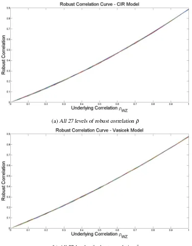
us a very good fit. So we will propose an exponential function to mapρWZ to ¯ρ:
¯
ρ=a[exp(bρWZ)−1] (4.14)
where a and b are fitted parameters and ˆρ denotes the estimate of ¯ρ. So there are only 2
parameters to estimate.To fit the curve, we divide the interval[0,1]intoK small subintervals and define
δρ =
1 K, ρ
i
W Z=iδρ, i=1,2,· · ·,K.
For each givenρWZi , we run the simulations to generate the exposures and default probabilities
to calculate ¯ρiusing formula (3.11). Then we fit the curve with the ¯ρi’s by estimating the values ofa,bby least square method.
We use two measures to test the accuracy of our approach. First we consider the relative
error of the ratio at each level ofρWZ, which is defined as
ερWZ≡
CVAFratio−CVAS ratio CVASratio
.
It’s easy to see that this relative error is also the relative error of CVA. We check the maximum
ερWZ across allρWZlevels to see if our approach is accurate enough. The other measure we use
is the mean squared error (MSE) which is defined as
MSE ≡ 1 K
K
∑
i=1 h
CVAFratio(ρWZi )−CVASratio(ρWZi )
i2 .
As discussed in the previous section we calculateCVAINDwith 100,000 paths and deriveµV(ti),
µq(ti),σV(ti)andσq(ti). First we calculate the robust correlations forK=20, i.e., at the points whereρWZi equals 0.05, 0.1, . . . , 0.95, 1. At each point we generate 10,000, 30,000, 50,000 or
70,000 paths to test if we need more paths to fit a robust correlation curve that can be used in
our approach. From Tables 4.1 and 4.2, we can see that 10,000 paths is good enough.
results are given in Tables 4.3 and 4.4. For comparison purpose, in Fig. 4.3 , the CVA ratio curves
derived using the full simulation and using our approach are plotted. Obviously increasing the
fitting points ofρWZ may not give us more benefit. So in this case, we conclude that 5 points ofρWZ between 0 and 1 is adequate to fit a robust correlation curve. Thus the total paths we generate are 150,000. But one can get the CVA with anyρWZ between 0 and 1.
Throughout the rest of this paper, we fit the robust correlation curve with 5 points of ρWZ and 10,000 paths at eachρWZ. In the next section, we will test the robustness of the approach and perform some sensitivity analysis and extreme scenarios analysis.
4.5
Sensitivity Analysis and Extreme Scenarios
To test the robustness of our method, we first consider small perturbations of the parameters
and investigate the range of change for the robust correlation ¯ρ. Here we perturb all 3 interest
process parameters,κr,θr andσr, by±10% of their current level. We denote the current level as ‘MMM’. A -10% level is denoted as ‘L’ and +10% as ‘H’. Since we have 3 input parameters,
there are 33possible levels to examine. We want to see if it is possible to fit the robust correlation
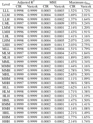
curve once for the ‘MMM’ level and reuse it for all other levels.With the fitted curve for level ‘MMM’, we calculate adjusted R-squares for all 27 levels to check the accuracy of fit. The
statistics and measures of accuracy are in Table 4.5. From this table, we can see that the adjusted
R2statistics are very close to 1, which means the fitted curve can represent all other levels very
well. The accuracy measures indicate the fitted robust correlation can be used to calculate CVA
and capture WWR with relative error below 4% in magnitude. Therefore, instead of regenerating
ρ(ti)and calculating ¯ρ for all levels, we can just use ˆρ fitted from level ‘MMM’ to represent all other levels. We can replace ¯ρ with ˆρ and plug it to our formula in Eq. 3.13, CVA ratio
curves for all 27 levels can be calculated easily without losing much accuracy. Such analysis can
also be performed against parameters forXtorht process. However, a company’s credit quality information is usually updated quarterly or monthly and we assume that theXt orht process is estimated less frequently unless there is a credit event. A credit event can trigger unwinding
of transactions, which will definitely impact the CVA calculation. One should always re-fit the
The previous experiments may not reveal which input parameter has greater impact on the
CVA ratio. Also we need to know how sensitive ¯ρ and Cp are with respect to each input parameter. We start from level ‘MMM’. Every time we only perturb one input parameter
of the interest rate process within a certain range. The range we use for κr, βr and σr are
κr∈[0.05,0.5],βr ∈[0.04,0.4]and σr∈[0.04,0.4]respectively. These ranges are all equally spaced. Table 4.6 shows the sensitivity of robust ¯ρ whenρWZ is 1. Fig. 4.4 and 4.5 show the value ofCpfor all different parameter levels.
Table 4.6 contains the value of ¯ρ whenρWZis 1 where ¯ρ differs most. We can see that except in
the case a CIR model is assumed andσrchanges, the maximum difference of ¯ρ in percentage is
below 6% and we don’t have to re-fit our curve. This means for partial perturbation, the robust
correlation can be reused without losing too much accuracy unless the volatility of CIR model
changes a lot.
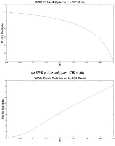
From Fig. 4.4 and 4.5 we observe similar trends for both CIR and Vasicek models. Cp de-creases asκr orβr increases. A largerκr draws the interest rate to its mean reverting level faster and this reduces the volatility of the exposure and the numerator ofCp given in Eq. 3.12. A larger βr leads to a higher mean reverting level and increases the mean of exposure and the denominator ofCp. A largerσr means more volatile and increases the volatility of the exposure and the numerator ofCp. We view the jump ofCpin Fig. 4.5a as simulation error. The sensitivity analysis ofCptells us that portfolios with differentCpshould not be treated the same when we consider WWR. Holding everything else the same, a more volatile portfolio has more risk to be
amplified and it needs a bigger adjustment factor. Note here that people don’t have to worry
about this when they use our model sinceCpis derived every time whenCVAINDis calculated via full simulation. This will not add any computational effort.
In the real world the long term mean reverting level is usually stabler than the other two inputs, so we further examine two more extreme scenarios. Notice that for a given level of
βr, the interest rate process is less volatile whenκr is large andσr is small. Our ‘low volatile’ scenario usesκr =0.5,βr =0.1 andσr=0.04 and ‘high volatile’ scenario takesκr=0.05,
to derive the CVA ratio curve and check its accuracy. Fitted parameters, accuracy measures,Cp and maximum CVA ratio are given in Table 4.7.
As a result from the extreme scenario analysis the CVA ratio can vary from 2.7434 to 4.1460.
BothρWZ andCpchange a lot. See Table 4.7. Therefore in the situation where dramatic change of the underlying interest rate process, a reusable robust correlation curve is not guaranteed and
thus one should re-fit the curve for the subsequent analysis.
4.6
Confidence Interval for CVA and CVA Ratio
The correlation between the exposures and the default probabilitiesρWZ, plays a key role in the CVA calculation. However, it is not directly observable from the market and the risk manager
has to estimate its value. The correlation may change from time to time, and the risk manager
may just have a range of the correlation with certain confidence level. On the other hand, to
estimate the CVA with a different correlation levelρWZ, the risk manager needs to run a full simulation. So to get a confidence interval for CVA, a risk manager may need to repeat the
full simulation many times to get the distribution of the CVA to obtain the confidence level.
On the other hand, in our approach, from the Eq. 3.14, we can see that, if the risk manager has a confidence interval about ¯ρ, she can get the confidence internal for CVA immediately.
If she has a confidence interval forρW Z instead of the robust correlation ¯ρ, by virtue of the monotone property of the mapping fromρW Z to ¯ρ, we can use the Eq. 3.14 and the values of ¯ρ corresponding to the two ending points of the confidence interval forρW Z to obtain the confidence interval for the CVA.
With our proposed method, we only need to run the simulations with computational efforts of
150,000 paths in this particular study case to generate the whole CVA profile forρWZ∈[0,1]. Not only it is easy to obtain the confidence interval, but it is also convenient to obtain the CVA for any correlation level very quickly. For a different level of ρWZ, we can use the formula (4.14) to obtain ˆρ then plug it into Eq. 3.13 to obtain the new CVA ratio and then use formula
(3.14) to obtain the CVA under the new correlation level. No need to run any simulations for
confidence interval is constructed. If we need 100 CVA values to construct the distribution of
CVA or to construct a confidence interval, we at least reduce the computational burden by 98.5%.
Finally, although ρWZ must be specified to perform the simulations to describe the WWR, it is more nature to consider the robust correlation ¯ρ instead ofρWZ. From our definition of ¯ρ, we can see that it describes the average correlation coefficient of the exposures and the default
probabilities. So if a risk manager has a view on the correlation, it should be described by ¯ρ
instead of ρWZ. Further, it makes more sense to build a confidence level of CVA based on a confidence level of ¯ρ instead of a confidence level ofρWZ.
4.7
Implementation Guide
Based our approach and numerical studies, we propose a step-by-step guide for CVA calculation.
Consider a risk manager who needs to calculate CVA with WWR. We assume that the risk
manager already have adapted her interest rate model and the default probability model, and
she need to calculate the CVA under different correlation levels. In other words, we assume
that the risk manager needs to calculate CVA under different level ofρW Z forρW Z ∈[0,1]. The step-by-step guide for CVA calculation is as follows:
Step 1. Run a full simulation (e.g. 100,000 paths) and use Eq. 4.11 to getCVAIND and use Eq. 3.12 to calculateCp;
Step 2. Choose a grid of 5 values ofρWZi , e.g. 0.2,0.4,0.6,0.8,1.0 and for each of them calculate
¯
ρiusing Eq. 3.11 with 10,000 paths;
Step 3. Fit a robust correlation curve given by Eq. 4.14;
Step 4. For any given value ofρW Z ∈[0,1], calculate ¯ρforρWZ using the fitted curve.
Step 5. ApplyCVAIND,Cpand ¯ρ into equation Eq. 3.14 to getCVAand its confidence interval;
From the results shown in Section 4.5, the model can be used without a full simulation if one of
the following robust criteria is satisfied:
i. The input parameters deviate from current level by no more than 10%;
ii. In the case of Vasicek model, if the parameters change in the following range: κr ∈
[0.05,0.5],βr∈[0.04,0.4]andσr∈[0.04,0.4].
iii. In the case of CIR model, if the parameters change in the following range:κr∈[0.05,0.5],βr∈
[0.04,0.4]andσrdoesn’t change more than 10%.
From this step-by-step algorithm, we can see that if a risk manager obtains a confidence interval
for the correlation ρW Z, she just needs to follow Step 4-6 for the maximum value and the minimum values ofρW Z to build the confidence interval for CVA. However this algorithm is not a recipe for any situations without caution. When extreme market scenarios or credit events with
the counterparty occur, a full simulation needs to be performed to reestablish the foundation of
Table 4.1 Fitted parameters and accuracy with 20ρWZpoints and different number of paths
-CIR model
Number of paths at eachρWZ
a b Adjusted R2 MSE Maximum
ερWZ
10,000 1.0272 0.6267 0.9999 0.0002 1.63%
30,000 1.0223 0.6273 0.9998 0.0001 1.69%
50,000 1.0085 0.6339 0.9999 0.0001 1.67%
70,000 1.0287 0.6245 0.9999 0.0001 1.70%
Table 4.2 Fitted parameters and accuracy with 20ρWZpoints and different number of paths
-Vasicek model
Number of paths
at eachρWZ a b Adjusted R
2 MSE Maximum
ερWZ
10,000 1.5091 0.4579 0.9999 0.0001 1.14%
30,000 1.5319 0.4524 0.9998 0.0001 1.21%
50,000 1.4717 0.4678 0.9999 0.0001 1.11%
70,000 1.4401 0.4762 0.9999 0.0001 1.05%
Table 4.3 Fitted parameters and accuracy with 10,000 paths and different number ofρWZ
points - CIR model
Number of
ρWZ points
a b Adjusted R2 MSE Maximum
ερWZ
5 1.0195 0.6321 0.9998 0.0002 1.44%
10 1.1040 0.5931 0.9998 0.0002 1.50%
20 1.0272 0.6267 0.9999 0.0002 1.63%
Table 4.4 Fitted parameters and accuracy with 10,000 paths and different number ofρWZ
points - Vasicek model
Number of
ρWZ points
a b Adjusted R2 MSE Maximum
ερWZ
5 1.3791 0.4934 0.9999 0.0001 1.16%
10 1.4522 0.4721 0.9999 0.0001 1.25%
Table 4.5 Goodness of fit statistics and accuracy using the robust correlation curve fitted at level ‘MMM’
Level Adjusted R
2 MSE Maximum
ερWZ
CIR Vasicek CIR Vasicek CIR Vasicek
LLL 0.9998 0.9999 0.0003 0.0003 1.52% 1.72%
LLM 0.9996 0.9999 0.0004 0.0005 1.69% 2.01%
LLH 0.9996 0.9999 0.0001 0.0002 1.37% 1.64%
LML 0.9997 0.9999 0.0003 0.0009 1.95% 3.24%
LMM 0.9996 0.9999 0.0006 0.0001 2.14% 1.20%
LMH 0.9996 0.9999 0.0002 0.0003 1.43% 1.91%
LHL 0.9998 0.9999 0.0001 0.0001 1.41% 1.16%
LHM 0.9998 0.9999 0.0004 0.0005 2.07% 2.10%
LHH 0.9997 0.9999 0.0009 0.0013 2.03% 2.75%
MLL 0.9998 0.9999 0.0002 0.0004 1.51% 1.79%
MLM 0.9997 0.9999 0.0009 0.0004 2.43% 1.84%
MLH 0.9997 0.9999 0.0002 0.0001 1.89% 2.00%
MML 0.9999 0.9999 0.0001 0.0001 1.45% 1.34%
MMM 0.9998 0.9999 0.0002 0.0001 1.44% 1.16%
MMH 0.9997 0.9999 0.0003 0.0002 1.78% 1.59%
MHL 0.9999 0.9999 0.0006 0.0001 2.65% 2.30%
MHM 0.9998 0.9999 0.0001 0.0001 1.11% 1.09%
MHH 0.9997 0.9999 0.0003 0.0002 1.96% 1.58%
HLL 0.9999 0.9999 0.0002 0.0002 1.62% 1.61%
HLM 0.9998 0.9999 0.0003 0.0001 1.71% 1.38%
HLH 0.9998 0.9999 0.0002 0.0001 1.21% 1.19%
HML 0.9999 0.9999 0.0003 0.0003 1.47% 1.50%
HMM 0.9999 0.9999 0.0002 0.0001 1.41% 1.41%
HMH 0.9998 0.9999 0.0001 0.0001 1.14% 1.08%
HHL 0.9999 0.9999 0.0003 0.0001 2.21% 1.49%
HHM 0.9999 0.9999 0.0003 0.0002 1.77% 1.65%
Table 4.6 ¯ρ ranges with perturbed input parameters Input
parameter
Parameter range
CIR Vasicek
Min ¯ρ Max ¯ρ % change Min ¯ρ Max ¯ρ % change
κr 0.05-0.5 0.8815 0.9337 5.92% 0.8690 0.9189 5.74%
βr 0.04-0.4 0.8623 0.8896 3.17% 0.8630 0.8773 1.66%
σr 0.04-0.4 0.7808 0.8914 14.16% 0.8366 0.8800 5.19%
Table 4.7 Fitted parameters, accuracy measures,Cpand CVA ratio
- extreme scenarios
Model Scenario a b Adj. R2 MSE Max.
ερWZ
Cp
Max. CVA ratio
CIR Low Vol 1.1454 0.5980 0.9993 0.0003 2.00% 1.8595 2.7434 High Vol 0.4109 1.0452 0.9982 0.0008 2.35% 4.1520 4.1460
Vasicek Low Vol 1.4592 0.4921 0.9997 0.0004 2.47% 1.6303 2.5122 High Vol 2.2641 0.3078 1.0000 0.0002 2.12% 1.8312 2.4943
(a)Robust correlation curve - CIR model
(b)Robust correlation curve - Vasicek model
(a)CVA ratio curve - CIR model
(b)CVA ratio curve - Vasicek model
(a)Profile multiplier with perturbedκr
(b)Profile multiplier with perturbedβr
(c)Profile multiplier with perturbedσr
(a)Profile multiplier with perturbedκr
(b)Profile multiplier with perturbedβr
(c)Profile multiplier with perturbedσr
(a)
(b)
(a)
(b)
(a)
(b)
(a)All 27 levels of robust correlationρ¯
Chapter 5
CVA DWR Multiplier Decomposition as A
Bridge
5.1
The Hull and White Model
In the case of WWR, when the dealer’s exposure is high the default probability of a counterparty
is also high. RWR takes the opposite side. The usual approach models DWR by calculating
conditional exposure. While Hull and White have proposed a different approach and do the
reverse. They change the calculation ofq(t)so that the evolution ofq(t)is related to that of V(t), whereV(t)can be the value of portfolio at timet.
Hull and White define the conditional default probability by linking the hazard rate, h(t), to the underlying future value of the portfolioV(t). Conditional on no earlier default, the probability of default in any small period∆t ish∆t. Viewing today as time 0, exp(−ht)is the probability of no default occurs before timet. If the hazard rate varies as a deterministic function of time then this no default probability is exp −Rt
0h(u)du
.
Hazard rates can change stochastically and are not directly observable from the market. But
following relationship must be satisfied E exp − Z t 0
h(u)du
=exp[−s(t)t], (5.1) wheres(t)is the counterparty credit spread with maturityt; 0 recovery rate is assumed. In a Monte Carlo simulation, assuming the discretization is equally spaced, Eq. 5.1 is
E "
exp(− j
∑
i=1 hi∆t)
#
=exp(−sjtj), (5.2)
wherehiandsjareh(ti)ands(tj)respectively. Hull and White assume
hi=g(V(ti)) =exp(ai+bV(ti)), (5.3) wherebis a constant that measures the amount of DWR,ai is a function ofti that should be calibrated with Eq. 5.2. The detailed procedure of this calibration is given in Hull and White.
Our discussion in the next section will be based on their model.
5.2
Analytical Results
In this section, we make some assumptions and derive some analytical results to have some
insights of Hull and White model.
We assume the following assumptions hold:
1. There areKtime periods;
2. tj = j∆t for j=1,2, . . . ,Kand∆t= 2521 ;
3. The profit and loss attj is denoted asXj;
5. Suppose the initial value of the portfolio is a positive constantV0;
6. The observed credit spread with maturitytjissj; 7. t0,X0ands0are all 0;
8. Recovery rate and discount rate are 0;
9. The exposure at timetjisVj andVj=V0+∑ij=1Xi; 10. For all j, the probability ofVjfalls below 0 is negligible.
We define the hazard rate at timetjashj. Following Hull and White framework,hjis a function ofVjand
hj=g(Vj) =exp(aj+bVj), (5.4) wherebis a predetermined constant andaiis time dependent and should be calibrated so that
E "
exp(− j
∑
i=1 hi∆t)
#
=exp(−sjtj) We approximate the left-hand side of the above equation with
E "
exp(− j
∑
i=1 hi∆t)
#
≈1−E
"
∆t
j
∑
i=1 hi
#
(5.5)
Then the market implied probability of default between timetj−1andtj, denoted asCj, is
Cj≡exp(−sj−1tj−1)−exp(−sjtj)
=E "
exp(− j−1
∑
i=1 hi∆t)
#
−E
" exp(−
j
∑
i=1 hi∆t)
# ≈E " ∆t j
∑
i=1 hi
#
−E
"
∆t
j−1
∑
i=1 hi
#
=Ehj∆t
HenceCj’s can be expressed in terms of the expectation of hazard rate times∆t and we have
E[hj∆t] =Cj. (5.7)
In Appendix B, we use some numerical examples to show the error of this approximation is
acceptable.
From the definition ofhj,
E[hj∆t] =exp(aj−aj−1)E[hj−1∆texp(bXj)]. (5.8) From Eq. 5.8 one can see
exp(aj−aj−1)E[exp(bXj)] = Cj
Cj−1. (5.9)
CVA with independent exposure and default probability can be expressed as
CVAIND=E "
K
∑
j=1 VjCj
#
=E "
K
∑
j=1
Cj(V0+
j
∑
i=1 Xi)
#
=
K
∑
j=1
Cj V0+
j
∑
i=1 EXi
!
=
K
∑
j=1
Cj V0+ j
∑
i=1
µi !
.
(5.10)
CVA with DWR is
CVADW R=
K
∑
j=1
EVjhj∆t
=
K
∑
j=1 E
" V0+
j
∑
i=1 Xi
! hj∆t
# .
We show
E "
V0+ j
∑
i=1 Xi
! hj∆t
#
=Cj "
V0+ j
∑
i=1
(µi+bσi2)
#
(5.12)
by induction.
SinceV0is a constant and by Eq. 5.7, it is enough to show
E " j
∑
i=1 Xihj∆t
#
=Cj j
∑
i=1
(µi+bσi2) (5.13)
Stein’s Lemma:
Suppose X follows N(µ,σ2). Further assumegis a function for which bothE[g(X)(X−µ)]
andE[g0(X)]exist. Then
E[g(X)(X−µ)] =σ2E[g0(X)]
E[g(X)X] =σ2E[g0(X)] +µE[g(X)].
(5.14)
Following our assumptions and the definition of function g given by Eq. 5.4, we know the conditions of Stein’s Lemma are satisfied.
First let’s check when j=1
E[X1h1∆t] =E[X1exp(a1+bX1)∆t]
= (µ1+bσ12)E[h1∆t]
= (µ1+bσ12)C1.
Eq. 5.13 holds. Next, let’s assume Eq. 5.13 holds for j=n−1 and that is E
" n−1
∑
i=1
Xihn−1∆t
#
=Cn−1 n−1
∑
i=1
Then we move on to j=n E
" n
∑
i=1 Xihn∆t
#
=E "
(
n−1
∑
i=1
Xi+Xn)exp(an−an−1)exp(bXn)hn−1∆t #
=exp(an−an−1)E[exp(bXn)]E "
n−1
∑
i=1
Xihn−1∆t
#
+exp(an−an−1)E[Xnexp(bXn)]E[hn−1∆t]
=exp(an−an−1)E[exp(bXn)]E "
n−1
∑
i=1
Xihn−1∆t
#
+exp(an−an−1)E[exp(bXn)](µn+bσn2)E[hn−1∆t]
Taking Eq. 5.7, Eq. 5.9 and Eq. 5.15 to the right-hand side of the above equation we have
E "
n
∑
i=1 Xihn∆t
#
=Cn n−1
∑
i=1
(µi+bσi2)
+ (µn+bσn2)E[hn∆t]
=Cn n−1
∑
i=1
(µi+bσi2)
+Cn(µn+bσn2)
=Cn n
∑
i=1
(µi+bσi2). Hence Eq. 5.13 holds for all j.
Thus CVA with DWR given by Eq. 5.11 can be expressed as
CVADW R= K
∑
j=1 Cj
" V0+
j
∑
i=1
(µi+bσi2)
#
So the CVA ratio is given by
CVAratio≡
CVADW R
CVAIND =1+b
∑Kj=1 h
Cj∑ij=1σi2
i
∑Kj=1
h
CjV0+∑ij=1µi
i. (5.17)
The above equation shows that the CVA ratio is a function of b, moments of exposures and the observed credit spreads. It is irrelevant withaj’s. This result is not surprising since allaj’s are calibrated such that the expectation of default probabilities match those implied by the observed
market credit spreads. Thus the information carried byaj’s should be embedded in b, moments of exposures and the observed market credit spreads. In other wordsaj’s should be functions of those factors.
Denote the means and variances of the exposure and default probabilities as follows
EVj=µV(tj), Var Vj
=σV2(tj), E
hj∆t=µPD(tj), Var hj∆t=σPD2 (tj). With our assumptions, the followings hold
µV(tj) =V0+ j
∑
i=1
µi,
σV2(tj) = j
∑
i=1
σi2, µPD(tj) =Cj,
σPD2 (tj) =C2j[exp(b2 j
∑
i=1
The first two equations above are relatively straight forward. The third one is a calibration
condition in Hull and White approach. The derivation of the fourth one follows
Ehj∆t
=E "
exp(aj)exp[b(V0+ j
∑
i=1 Xi)]∆t
#
=exp(aj)exp(bV0)exp b j
∑
i=1
µi+
b2∑ij=1σi2
2 !
∆t
=Cj.
(5.18)
Thus we have
exp(aj)∆t=Cjexp(−bV0) "
exp b j
∑
i=1
µi+
b2∑ij=1σi2
2
!#−1
. (5.19)
Next, let’s derive the second moment ofhj∆t
E(hj∆t)2= (∆t)2E
"
exp(2aj)exp[2b(V0+ j
∑
i=1 Xi)]
#
=exp(2aj)(∆t)2exp(2bV0)exp 2b j
∑
i=1
µi+2b2 j
∑
i=1
σi2
! .
(5.20)
Taking Eq. 5.19 into Eq. 5.20
E(hj∆t)2=C2jexp(b2
j
∑
i=1
σi2). (5.21)
Hence
σPD2 (tj) =E
(hj∆t)2−(Ehj∆t
)2=C2j "
exp(b2 j
∑
i=1
σi2)−1
# .
We now consider the correlation coefficient ofVjandhjdirectly, namelyρ(tj). For each time node, we have
ρ(tj) =
Cov(Vj,hj∆t)
σV(tj)σPD(tj)