DOI: 10.1534/genetics.110.116855
The Impact of Genetic Architecture on Genome-Wide Evaluation Methods
Hans D. Daetwyler,*
,†,1Ricardo Pong-Wong,* Beatriz Villanueva
‡,§and John A. Woolliams*
*The Roslin Institute and Royal (Dick) School of Veterinary Studies, The University of Edinburgh, Roslin EH25 9PS, United Kingdom,†Animal Breeding and Genomics Centre, Wageningen University, 6700 AH Wageningen, Netherlands,
‡Scottish Agriculture College, Edinburgh EH9 3JG, United Kingdom and§Departamento de Mejora
Gene´tica Animal, Instituto Nacional de Investigacio´n y Tecnologı´a Agraria y Alimentaria, 28040 Madrid, Spain
Manuscript received March 21, 2010 Accepted for publication April 7, 2010
ABSTRACT
The rapid increase in high-throughput single-nucleotide polymorphism data has led to a great interest in applying genome-wide evaluation methods to identify an individual’s genetic merit. Genome-wide evaluation combines statistical methods with genomic data to predict genetic values for complex traits. Considerable uncertainty currently exists in determining which genome-wide evaluation method is the most appropriate. We hypothesize that genome-wide methods deal differently with the genetic architecture of quantitative traits and genomes. A genomic linear method (GBLUP), and a genomic nonlinear Bayesian variable selection method (BayesB) are compared using stochastic simulation across three effective population sizes and a wide range of numbers of quantitative trait loci (NQTL). GBLUP had
a constant accuracy, for a given heritability and sample size, regardless of NQTL. BayesB had a higher
accuracy than GBLUP whenNQTLwas low, but this advantage diminished asNQTLincreased and when
NQTL became large, GBLUP slightly outperformed BayesB. In addition, deterministic equations are
extended to predict the accuracy of both methods and to estimate the number of independent chromosome segments (Me) andNQTL. The predictions of accuracy and estimates ofMeandNQTLwere
generally in good agreement with results from simulated data. We conclude that the relative accuracy of GBLUP and BayesB for a given number of records and heritability are highly dependent onMe,which is a
property of the target genome, as well as the architecture of the trait (NQTL).
T
HE rapid progress and reducing costs of genome sequencing and high-throughput DNA techni-ques have led to a great interest in applying genome-wide evaluation methods to identify individuals of high genetic merit. Genome-wide evaluation uses associations of a large number of SNP (single nucleotide poly-morphism) markers across the whole genome with phenotypes to produce accurate estimates of breeding values (EBVs) for candidates to selection (Meuwissen et al. 2001). The accuracy of genome-wide selection (i.e.,selection based on genomic EBVs) is expected to be substantially higher than that of traditional best linear unbiased prediction (BLUP) selection, which is based on pedigree and phenotypic data (Daetwyler et al.
2008; Goddard2009; Hayes et al. 2009c). In addition,
genome-wide selection has the potential to reduce inbreeding rates because of the increased emphasis on own rather than family information (Woolliams et al. 2002; Daetwyler et al. 2007; Dekkers 2007).
Furthermore, the application of genome-wide evalua-tion approaches can significantly aid our understanding of quantitative trait genetic architecture.
The genome-wide evaluation methods suggested to date can be broadly categorized into groups according to whether there is an assortment of the SNP by magnitude of effect or contribution to the variance. One group treats SNP homogeneously and includes variants of genomic best linear unbiased prediction (GBLUP). This group includes a form of ridge regression (Meuwissen et al. 2001) and the use of a realized relationship matrix computed from the markers instead of the traditional pedigree matrix (NejatiJavaremiet al. 1997; Villanueva et al. 2005; Hayeset al. 2009c). Both approaches have
been shown to be equivalent (Habier et al. 2007;
Goddard 2009). A second group provides for
hetero-geneity among SNP contributions to the variance, with some contributions permitted to be large while the remainder are small, possibly zero. This assortment is helped by Bayesian approaches, which place priors on numbers of SNP with major contributions (e.g.,BayesA and BayesB; see Meuwissenet al. 2001, 2009; Leeet al.
2008), or with some penalty based on functions of the magnitude of effect for each SNP (e.g., Lasso; see Tibshirani1996; Yiand Xu2008) or with other
smooth-ing metrics (Longet al. 2007). A third group attempts to
reduce dimensionality by using principal components or partial least squares (Raadsmaet al. 2008; Solberg
1Corresponding author: Bioscience Research Division, Department of
Primary Industries, 1 Park Dr., Bundoora 3083, Victoria, Australia. E-mail: hans.daetwyler@dpi.vic.gov.au
et al. 2009) to identify an informative subset of SNP genotypes. The main two methods currently used in real data sets are a linear prediction method, GBLUP, and variants of nonlinear Bayesian variable selection ap-proaches such as BayesB.
In most simulated published data, the accuracy of BayesB outperformed that of GBLUP (e.g.,Meuwissen et al. 2001; Habier et al. 2007; Lund et al. 2009).
However, real data results have not consistently sup-ported this conclusion. Two reviews of empirical results in dairy cattle to date have shown that GBLUP and BayesB result in very similar accuracies for most traits (Hayeset al. 2009a; Vanradenet al. 2009). One reason
for the disagreement between simulated and real data results could be that the genetic architecture simulated is significantly different from what is found in real populations. Most studies published to date that com-pare methods using simulated architectures have con-sidered only 50 or fewer QTL affecting the trait (e.g.,
Meuwissenet al. 2001; Habieret al. 2007; Lundet al.
2009). In this article we hypothesize that the relative utility of genome-wide evaluation methods depends significantly on both the genomic structure of the population and the genetic trait architecture.
The main objective of this study was to compare a linear method, GBLUP, and a nonlinear variable selec-tion method, BayesB, using simulated data across a range of population and trait genetic architectures to further understand the mechanics of genome-wide evaluation methods. An important secondary objective was to extend deterministic prediction models to pre-dict the accuracy of both methods. Theoretical models complement stochastic simulation by helping the un-derstanding of the factors involved in genome-wide evaluation performance and, in return, stochastic sim-ulation is used to confirm theoretical derivations.
METHODS
Theoretical development: Daetwyler et al. (2008)
derived equations for predicting the accuracy of a simple least-squares genome-wide evaluation approach for continuous and dichotomous traits. The original formula for genome-wide accuracy for a continuous trait is rg ˆg¼
ffiffiffiffiffiffiffiffiffiffiffiffiffiffiffiffiffiffiffiffiffiffiffiffiffiffiffiffiffiffiffiffiffiffiffiffiffiffiffiffiffiffi
ðNPh2Þ=ðNPh21nGÞ
p
, where rggˆ is the correlation between true and estimated additive genetic values (i.e.,accuracy),NPis the number of individuals in
the training population,h2is the heritability, andn
Gis the number of independent loci (Daetwyler et al.
2008). The accuracy was independent of how large the subset of loci was that make nonzero contributions. Thus, it did not matter whether there were many nonzero loci effects of small magnitude or only a few nonzero loci effects of large magnitude. In Daetwyler et al. (2008), the formulae were derived by considering the regression of phenotypes on one locus at a time as
loci were assumed independent. Therefore the formula will work for small numbers of dispersed loci in a genome but the accuracy will tend to zero asnGbecomes large; erroneously, because loci cannot be added inde-pendently in a finite genome due to linkage. Daetwyler et al. (2008) discussed that an empirical value for the number of independent chromosome segments (Mˆe)
could be used in place ofnG, becausenGwas assumed independent. Goddard(2009) also proposed accuracy
predictions for GBLUP, which used the concept of predicted Me. His derivation builds on work by
Visscher et al. (2006) in which the variance of
identi-cal-by-descent sharing for full sibs was developed and provides a prediction for Me, which is Me ¼ 2NeL/
log(4NeL), where L is the genome length in Morgans
(Goddard2009). SubstitutingMein place ofnGin the
original formula of Daetwyleret al. (2008) results in
rg ˆgG ¼
ffiffiffiffiffiffiffiffiffiffiffiffiffiffiffiffiffiffiffiffiffiffiffi NPh2
NPh21Me
s
; ð1Þ
which also predicts the accuracy of GBLUP. At no time does the argument moving from the original formula of Daetwyleret al. (2008) to Equation 1 depend on the
distribution of the effects of loci, so we come to the first hypothesis in this study that states that GBLUP accuracy is independent of the number of quantitative trait loci (NQTL) associated with the phenotypic trait.
Our second hypothesis was that the accuracy of BayesB whenNQTLis high would tend to that of GBLUP.
If our first hypothesis is confirmed, then the depen-dence of GBLUP onMeis an advantage at highNQTL,
even thoughNQTLmay be higher thanMe. Heuristically,
if GBLUP delivers accuracy as if there are aMenumber
of QTL, the benefit from prior information that there are approximatelyMe(or more) QTL is unclear given
Equation 1. On the other hand, it is a clear disadvantage ifNQTL,Mebecause GBLUP cannot adapt the model
to suit the data. In contrast, BayesB is a variable selection method that attempts to determine the ‘‘optimum dimensionality’’ given the data and prior information. WhenNQTLis high this optimum is likely to be Mein
both methods. Hence, the accuracy of BayesB at high
NQTLcan be predicted in the same way as GBLUP, but if NQTL,Me, variable selection may deliver an advantage
in accuracy because choosing a subset of variables will reduce the dimensionality of the model. Thus, substitut-ingNQTLforMeis likely to better predict the accuracy of
BayesB. This results in the following equation,
rg ˆgB ¼
ffiffiffiffiffiffiffiffiffiffiffiffiffiffiffiffiffiffiffiffiffiffiffiffiffiffiffiffiffiffiffiffiffiffiffiffiffiffiffiffiffiffiffiffiffiffiffiffi NPh2
NPh21minðNQTL;MeÞ
s
: ð2Þ
Further rearrangement of Equations 1 and 2 allows for empirical estimates of Me (Mˆe) to be made in the
ˆ
Me ¼ ðNPh2Þð1rg ˆ2gÞ=rg ˆ2g; ð3Þ
wherer2
g ˆgis the squared accuracy of estimates of genetic values using GBLUP or BayesB (whenNQTL$Me) for
individuals without phenotypes. Predicting Mˆe with
GBLUP requires molecular relatedness to be known, whereas this is not required when using BayesB. This result gives a further subhypothesis that the empirical
Meis predicted by the formula for independent
chro-mosome segments given by Goddard (2009). Also, if NQTL , Me, additional information on NQTL can be
gathered using BayesB accuracy because it can choose a subset of loci or variables, by applying the following formula:
ˆ
NQTL¼ ðNPh2Þð1rg ˆ2gBÞ=rg ˆ2gB: ð4Þ
Therefore, additional insight into quantitative traits can be gained by combining genome-wide evaluation and deterministic prediction. The accuracy of BayesB is of course influenced by the priors used in the analyses (especially priors on the proportion of loci with no effect); hence it is important to use appropriate priors to get accurateNˆQTL.
Simulations:Our study consisted of three main steps. First, populations of individuals were simulated to be in mutation drift equilibrium. Second, effects were as-signed to a number of QTL that were randomly selected from the whole set of segregating loci, and true genetic values and phenotypes were generated for each in-dividual. The third step consisted of the genetic evalua-tions of the individuals generated with both GBLUP and BayesB.
Populations and genome: Populations in mutation drift equilibrium were simulated by random mating individuals for many generations with recombination and mutation. The number of male and female parents was12Ne across generations. A total of 1000, 5000, and
10,000 generations were simulated until linkage dis-equilibrium and heterozygosity values were stable for
Ne¼200,Ne¼1000, andNe¼2000, respectively. In the
final generation, a set of training individuals (of variable size) in which the loci effects were to be estimated was generated by random mating. Using the same parents, a set of validation individuals of size equal to the training set was produced whose genetic values were to be predicted. In scenarios where the size of the training sets (NP) was larger than Ne, population size was
increased by increasing the number of offspring per mating in the final generation.
The total genome size was 10 M (10 chromosomes of 1 M each). In generation zero all individuals were com-pletely homozygous for the same allele and mutations were applied at a rate of 2.5 3 105per locus per meiosis
in the following generations. Mutations switched allele one to two and vice versa. The number of randomly dis-tributed mutations per chromosome was sampled from
a Poisson distribution with mean corresponding to the product of the number of loci per chromosome and the mutation rate. Similarly, recombinations per chromo-some were sampled from a Poisson distribution with a mean of one per morgan and were then randomly placed along the chromosome. Linkage disequilibrium (LD) statistics,i.e., R2(Hilland Robertson1968), between
adjacent segregating loci were averaged among all pairs exceeding a minor allele frequency of 0.05 and matched expectedR2values (Sved1971; Tenesaet al. 2007). Allele
frequency distributions were found to follow a U-shaped distribution.
The number of loci at the start of the simulation (generation zero) required several considerations con-cerned with obtaining an appropriate number of segregating loci (Ne) andNQTLin the final generation.
The realized relationship matrix used in GBLUP can be singular ifNLis less than the number of individuals in
the matrix (Vanraden2008), preventing the inversion
needed to compute solutions. Thus,NLat mutation drift
equilibrium was made larger than the maximum sum of training and validation individuals to be used, and a similarNLwas used across all scenarios. However, asNe
increased, the proportion of segregating loci in the last generation also increased and forNe¼200,Ne¼1000,
and Ne¼2000, approximately 0.04, 0.28, and 0.52 of
initial loci were segregating at mutation drift equilib-rium, respectively. This required the adjustment of the number of initial loci. Across all scenarios, NL varied
between 4576 and 4721 loci (SE,9.5 loci). To obtain
NQTL,Mein a random mating population, as derived by
Goddard(2009), was used as a guide to allow
compar-isons to be made across Ne. The following NQTL
scenarios were simulated: 0.03, 0.05, 0.15, 0.30, 0.50, 0.75, and 1Me. Table 1 outlines the correspondingNQTL
for these proportions of Mefor the three Ne, whereas
Table 2 shows all scenarios that were carried out. Note that throughout this study our use of the terms ‘‘low’’ or ‘‘high’’ NQTL may refer to different actualNQTL across
the threeNebecauseNQTLwas scaled to be proportional
toMe(Table 1).
The desired NQTL were randomly chosen from NL.
True allele substitution effects were sampled fromN(0, 1). True breeding values for 2NP (i.e., training and
validation set) individuals were calculated for each QTL as 2(1pj)bj(wherepjis the major allele frequency at
TABLE 1
Number of QTL simulated for each proportion of independent chromosome segments (Me) for three values of effective population size (Ne)
Ne 0.03Me 0.05Me 0.15Me 0.3Me 0.5Me 0.75Me 1Me
200 13 22 67 133 223 334 445
locusj),2pjbj, and ((1pj)pj)bjfor the major and minor homozygote and heterozygote genotype, respec-tively (Falconer and Mackay 1996). Total breeding
values were obtained by summing overNQTL. Breeding
values were scaled to have the variance of h2 (i.e.,
phenotypic variance is 1). Phenotypic records were simulated for NP (training set) animals by adding
in-dependent environmental terms drawn fromN(0, 1h2)
to true breeding values. In addition, samplingbjfrom a Laplace (double exponential) distribution was investi-gated in scenario 4. The accuracy of both genome-wide evaluation methods was computed as the correlation between true and estimated breeding values.
GBLUP analysis: The evaluation with GBLUP ap-plied the following model, which was fit in ASReml (Gilmouret al. 1995):y¼m11Za1e, whereyis the
vector of phenotypic values,mis the population mean,Z
is an incidence matrix for random individual effects,ais a vector of random individual additive genetic values, and
eis the residual. Random effectsaandewere assumed normally distributed as Nð0;Gs2
aÞ and Nð0;Is 2 eÞ,
re-spectively, whereGwas the realized relationship matrix computed using the NL loci. In G, the relationship
between a pair of individuals was based on identical-by-state probabilities and included all training individuals with phenotypes and validation individuals without phe-notypes. The total allelic relationship at a locus between a pair of individuals was calculated as 0:5P2i¼1P2j¼1dij, wheredijis 1 if alleleiin the first individual is identical to allelejin the second individual and 0 otherwise. Averaging over loci as 0:5P2i¼1P2j¼1dij½NL
1
yields the numerator relationship between all individual pairs required forG
(NejatiJavaremi et al. 1997). Breeding values were
ob-tained by solving the mixed model equations (Henderson
1975).
BayesB analysis: We implemented a variant of the original BayesB (Meuwissen et al. 2001). The model
applied was y¼m11PNL
j¼1Xjbj1e, where m was the
mean,Xwas an incidence equal to1, 0, and 1 for 11,
12/21, and 22, respectively,b is the allele substitution effect for locus j, and e was the vector of residuals distributed asNð0;s2
eÞ. Allele substitution effects were
assumed to come for a mixture distribution where a proportion (p) had no effect and a proportion (1p) had effects distributed asNð0;s2
snpÞ.
The prior used formwas uniform, over a long range (i.e.,100s2
Pto1100s 2
P), and fors 2
ewas uniform (i.e.,0
to 1100s2
P), wheres 2
Pis the phenotypic variance of the
data set analyzed. The prior fors2
snp was taken from a
scaled inverted chi-square distribution of the form
s2
snp ys2x
2
y , wheres2represented the prior value for s2
snpandywas its degree of belief (Wanget al. 1994). A
weak prior was chosen to be 1 for bothyands2across all
scenarios. The influence of ours2ons2
snpestimates from
BayesB was investigated and was found to be small. A critical discussion of the impact of priors on BayesB can be found in Gianolaet al. (2009).
To test effect ofpon breeding value accuracy, two types of scenarios were carried out. In the majority of scenarios, 1pwas fixed to true values simulated for a particular scenario, 1 p ¼ NQTL[NL]1, which we call the
‘‘in-formed prior.’’ However, in scenario 8, 1pwas fixed to 57 QTL for allNQTLscenarios, 1p¼57 QTL[NL]-1,
which we term the low prior. While not done in this study, one could estimate 1pinstead of using a prior and this may be an advantage in real data with unknownNQTL
(e.g.,Pong-Wongand Hadjipavlou2010).
Our implementation of sampling loci variances was slightly different from that of Meuwissenet al. (2001).
They performed a haplotype analysis and therefore several haplotype effects would need estimating per locus and having more than one effect per locus required sampling of locus variances. In this study, biallelic loci were simulated and, because only one effect was estimated per locus, it was not necessary to sample a per-locus variance. This process of sampling from one variance is more similar to that of Xu(2003).
However, his implementation assumed all loci had an effect, which is comparable to BayesA of Meuwissen et al. (2001). In contrast, our model assumed that some loci will not have an effect (p), which is more similar to BayesB. In addition, while Xu(2003) used a naı¨ve prior
fors2
snp, we used an informative prior (i.e.,yands2¼1)
as proposed by TerBraaket al. (2005).
The length of the Gibbs chain was 105,000 iterations and the first 5000 iterations were discarded as burn-in. Estimates at every 20th iteration were stored as a sample resulting in a total of 5000 samples. Several analyses were carried out to test if the sampling protocol was appropriate. Autocorrelations of effects and estimated breeding values were found to be close to zero in stored samples, which showed that they were almost indepen-dent, so Monte Carlo error was,0.0003 in all scenarios (Geyerand Thompson 1992). This allowed for
short-ening of the chain length to 45,000 iterations (2000 samples) for scenarios with NP ¼ 2000 to reduce
TABLE 2
Parameter values for the simulated scenarios, whereNeis the effective population size;NPis the number of individuals in the training set;h2is the heritability; Prior is the prior
used forpin BayesB; andMeis the number of independent chromosome segments
Scenario Ne NP h2 Prior Me
1 200 200 0.3 Informed 445
2 200 1000 0.3 Informed 445
3 1000 1000 0.5 Informed 1887
4 1000 1000 0.3 Informed 1887
5 1000 1000 0.1 Informed 1887
6 1000 500 0.3 Informed 1887
7 1000 2000 0.3 Informed 1887
8 1000 1000 0.3 57 QTL 1887
running time. Furthermore, convergence was investi-gated by using a variety of starting values fors2in the
BayesB. Using different starting values resulted in nearly identical estimates ofs2
snpand breeding value accuracy
suggesting that our Gibbs chains were converging. In addition, a long chain of 160,000 iterations was run and
s2
snp estimates and accuracy values were very similar to
the shorter chain. While convergence cannot be guar-anteed in any MCMC study, evidence suggests that our MCMC protocol converged.
RESULTS
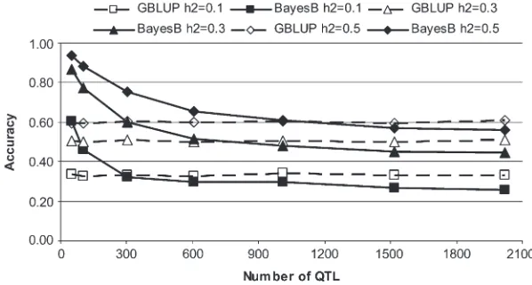
GBLUP accuracy:The accuracy of GBLUP for a given set of values forNPandh2stayed constant regardless of NQTLin all scenarios simulated (Figure 1 and Table 3).
This confirmed our first hypothesis. The constant accuracy results from the uniqueMeof a random mating
population, which, in turn, depends on Ne and L
(Goddard 2009). The plateau of GBLUP accuracy
increased when more phenotypic records were used in the estimation of breeding values and whenh2increased
(Figure 1). Samplingbjfrom a Laplace (double expo-nential) distribution resulted in the same GBLUP accuracy as sampling fromN(0, 1).
BayesB accuracy:In contrast to GBLUP, with BayesB the accuracy was highest at low NQTL and then
de-creased asNQTLincreased (Figure 1 and Table 3). Once NQTL was high, BayesB reached a plateau where the
accuracy does not decrease anymore despite increasing
NQTL. This plateau was observed in all BayesB scenarios
and the value of the accuracy at this plateau depended on Ne, h2, and NP (Tables 3 and 4). The plateau
decreased when Ne increased. An increase in h2 and NPinfluenced the accuracy in two ways: first, it raised the
overall accuracy in all NQTL scenarios, and second, it
slightly shifted the onset of the accuracy plateau to higherNQTL. Sampling effects from a Laplace
distribu-tion instead ofN(0, 1) raised BayesB accuracy slightly, but whenNQTLwas equal to 0.03MeorNQTL.0.5Meno
difference in accuracy was observed between sampling from both distributions.
The use of lowNQTLpriors for 1pyielded a lower
accuracy than informed priors (Table 2, scenario 8, and Figure 2). The gap between the accuracy of informed and low priors increased asNQTLincreased because the
proportion of the genetic variance explained by the low
NQTLprior became smaller.
Comparison of GBLUP and BayesB: The compari-son of GBLUP and BayesB leads to several key observa-tions. BayesB always performed better than GBLUP at low NQTL. However, as NQTL increased, the difference
between the two methods became smaller and eventu-ally both approaches achieved very similar accuracy. The
NQTLat which this equivalence occurred was increased
Figure 1.—Accuracy of GBLUP and BayesB (informed priors forp) in validation individuals for different numbers of QTL and heritabilities (h2) when the effective population size is 1000
and the number of individuals in the training set is 1000. SE,0.018 in all scenarios.
TABLE 3
Accuracy of GBLUP and BayesB (informed priors forp) for different effective population sizes (Ne), numbers of QTL expressed as proportions ofMe, and numbers of individuals in the training set (NP) when the heritability
is 0.3. SE,0.023 in all scenarios
Method Ne NP 0.03Me 0.05Me 0.15Me 0.3Me 0.50Me 0.75Me 1Me
GBLUP 200 200 0.405 0.450 0.429 0.414 0.444 0.416 0.398
1000 1000 0.505 0.501 0.508 0.502 0.507 0.501 0.511
2000 2000 0.575 0.579 0.571 0.568 0.571 0.571 0.568
BayesB 200 200 0.739 0.649 0.463 0.400 0.398 0.365 0.344
1000 1000 0.865 0.772 0.601 0.516 0.480 0.451 0.445
with increasingNe,NP, andh2(Figure 1 and Tables 3 and
4). Once NQTL increased past the equivalence point,
BayesB had a slightly lower accuracy than GBLUP and settled at a constant accuracy (Table 3). The difference between GBLUP and BayesB at high NQTL decreased
whenNPwas increased. Sampling effects from a Laplace
instead of a Normal distribution did not affect these general trends.
In Figure 2, the maximumx-value ofNQTLplotted is
equal to the predictedMefrom Goddard (2009) and
one observes that BayesB accuracy approaches the plateau and becomes similar to GBLUP accuracy well belowMe. A first inspection therefore suggests that the
second hypothesis does not hold. However the argu-ment for the second hypothesis is based upon the empiricalMˆe.Mˆe calculated with Equation 3 for h2 ¼
0.1, 0.3, and 0.5 by averaging over the values ofNQTL
gives values of 890, 900, and 700. In this context, hypothesis 2 is shown to be broadly valid, in that superiority of BayesB over GBLUP disappears when
NQTL approaches Mˆe, although there is a trend for
BayesB accuracy to become similar to GBLUP accuracy sooner than Me. These observations held for other
scenarios. The comparison between Me and Mˆe is
addressed in more detail below.
Decay in accuracy: The decay in accuracy between training and validation individuals was also greater for GBLUP than that of BayesB at lowNQTL (Table 4) as
observed by Habier et al. (2007). However, this trend
diminished asNQTLincreased and the decay of accuracy
reached similar levels in both methods at highNQTL.
Predictions of accuracy:Figure 3 shows the accuracies of GBLUP and BayesB predicted with Equations 1 and 2, respectively, and the accuracies from simulations in the validation set. Predictions of GBLUP and BayesB (at high
NQTL) accuracy were generally accurate. The accuracy of
the predictions was highly dependent onMe. In BayesB,
the drop in accuracy asNQTL increased was predicted
well. Equation 2 tended to overpredict BayesB accuracy, particularly in scenarios where NQTL was a low
pro-portion ofMe, using Goddard(2009), and lowh2andNP.
Empirical Mˆe and NˆQTL:We estimatedMeusing the
accuracy of GBLUP or BayesB (when NQTL ¼ Me)
(Equation 3). When GBLUP accuracy was used, we averaged the accuracy across allNQTL scenarios
simu-lated for a given set of values forh2andN
P. This was done
for each population replicate to obtain a standard error. It is a subhypothesis thatMeas predicted by Goddard
(2009) approximates Mˆe. Empirical estimates of Me
using GBLUP were always lower than those using BayesB (Table 5) due to the higher GBLUP accuracy whenNQTL
is high. The estimates using BayesB accuracy were more variable than GBLUP as shown by the larger SE of BayesB. A general trend was apparent showing thatMˆe
increased as NPincreased, which suggests thatMˆe has
not reached a bound; however, the change inMˆeis small
in relation to the difference fromMe. Furthermore,Mˆe
does not increase linearly withNPand this may indicate
that it may be approaching asymptotic values.
The number of QTL controlling the trait (NQTL) was
estimated using Equation 4 with reliability values from BayesB when NQTL , Me. As shown in Figure 4 for
scenario 7, the estimatedNQTLdo follow the actualNQTL
well and are predictive of the trend. Empirical NˆQTL
were better estimated with higher NP. Note that
in-correct priors will reduceNˆQTLaccuracy.
DISCUSSION
We have compared GBLUP and BayesB at various population and trait genetic architectures and at various
NP. We demonstrated that GBLUP had a constant
accuracy, for a given NP and h2, regardless of NQTL.
The accuracy of BayesB was greatest at low NQTL,
decreased with increasingNQTL, and eventually reached
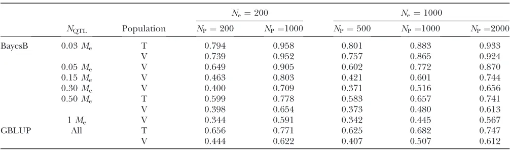
a lower accuracy plateau below which the accuracy did TABLE 4
Accuracy of GBLUP and BayesB (informed priors forp) in training (T) and validation (V) individuals for different effective population sizes (Ne), numbers of QTL (NQTL) expressed as proportions ofMe, and numbers of individuals in the
training set (NP) when the heritability is 0.3. SE,0.023 in all scenarios
Ne¼200 Ne¼1000
NQTL Population NP¼200 NP¼1000 NP¼500 NP¼1000 NP¼2000
BayesB 0.03Me T 0.794 0.958 0.801 0.883 0.933
V 0.739 0.952 0.757 0.865 0.924
0.05Me V 0.649 0.905 0.602 0.772 0.870
0.15Me V 0.463 0.803 0.421 0.601 0.744
0.30Me V 0.400 0.709 0.371 0.516 0.656
0.50Me T 0.599 0.778 0.583 0.657 0.741
V 0.398 0.654 0.373 0.480 0.613
1Me V 0.344 0.591 0.342 0.445 0.567
GBLUP All T 0.656 0.771 0.625 0.682 0.747
not fall even whenNQTLwas further increased. BayesB
has an advantage over GBLUP at low NQTL, but this
advantage decreased as NQTL increased and it finally
diminished completely or, in some cases, the advantage switched to GBLUP depending onNeandNP. The point
at which GBLUP and BayesB accuracy became equal was related to the empirical number of independent seg-ments estimated from the GBLUP accuracy,Mˆe, which
was less than the theoretical prediction ofMeprovided
by Goddard (2009). It is clear from this study that
quantifying the superiority of GBLUP over BayesB or vice versa depends upon three sets of attributes: the population genome structure (e.g., Ne), the trait genetic
architecture (e.g., NQTL,h2), and the size of the training
set. Superiority is, therefore, not a property of the method and general statements to that effect should be avoided. Furthermore, we have proposed and tested equations for the prediction of GBLUP and BayesB accuracy and the estimation of Mˆe and NˆQTL. Our
predictions follow achieved GBLUP and BayesB accu-racy well. EmpiricalMˆe values seem to be approaching
an asymptote with increasing NPand our estimates of ˆ
NQTLfollow the trend of trueNQTL.
The constant accuracy of GBLUP, for a givenh2and NP, confirmed our first hypothesis and clearly shows that
this accuracy depends crucially on genomic properties, and not on properties of the trait, and is summarized in the concept ofMe. In turn,Mewill depend onNeandL,
which can be viewed, in the short term, as constants in a random mating population (Goddard 2009). In a
wider sense, Me and the more commonly known
haplotype blocks are both measures resulting from population history and as such are related, although not interchangeable. Haplotype blocks are physical segments of the genome within which haplotype di-versity is low, bounded by areas where evidence for historical recombination exists (e.g., Goldstein2001;
Gabrielet al. 2002; Frazeret al. 2007). While haplotype
blocks are a physical measure,Meis a more statistical
concept related to the behavior of the genome in genomic evaluations. It is theoretically derived from
variation in relationship between relatives and from the continuum of variation in linkage disequilibrium across the genome (Goddard 2009). Both the number of
haplotype blocks and Me increase with increasing Ne
and in close relatives haplotype blocks will be long and
Mewill be small (Hayeset al. 2009c). It should be noted
that the dependence of GBLUP on Meshown in this
study does not support the conclusion that GBLUP assumes an infinitesimal model in which there are a very large number of genes each contributing a small portion to the genetic variance. In fact, GBLUP is indifferent toNQTL, unlessNQTLis very small (i.e.,one
or,10 QTL; unpublished results), as demonstrated in this study.
While it is clear that in GBLUP the accuracy depends onMeand not onNQTL, in BayesB the accuracy depends
on the interplay of both features of genetic architecture (NQTLandMe). Our results follow our second
hypoth-esis that the behavior of BayesB accuracy at highNQTLis
similar to that of GBLUP. The accuracy of BayesB declines as NQTL increases and eventually becomes
similar to GBLUP asNQTLincreases. The point at which
this occurs approaches Me with increasing NP.
There-fore, we show that the accuracy of BayesB at highNQTLis
also dependent on Mejust like in GBLUP. This is also
supported by the accuracy plateau being observed across similar proportions of Meand that near
equiva-lence is approximated closely byNQTL¼Mˆe, whereMˆeis
the empirical estimate of Me obtained from GBLUP.
Therefore, the plateau is not a function of actualNQTL
but of Me. Another argument for Mˆe to be a major
determinant in BayesB accuracy at high NQTLis that it
can be accurately predicted with Equation 3. In addi-tion, a recent study of Barley using real data has also shown that GBLUP accuracy exceeded that of BayesB whenNQTLwas large (Zhonget al. 2009).
additional step is involved in which for each locus it is estimated if the locus has an effect or not. The fact of choosing a near-correct subset of loci with effect with BayesB increases accuracy but there is also an error associated with determiningp, which depends on NL.
WhenNQTL,Methe advantage of choosing a subset is
clear but whenNQTL$Methis diminishes (heuristically,
it is likely that each independent segment contains QTL). Thus, under the latter scenario, GBLUP per-forms slightly better than BayesB. This argument is further supported by the decreasing difference in accuracy between GBLUP and the BayesB accuracy plateau at high NQTL when NP is increased, because
BayesB can identify the loci with effect better with more information.
The use of QTL effects sampled from a Laplace distribution instead of a Normal distribution resulted in no quantitative change to GBLUP accuracy and in only minor changes in accuracy to BayesB. Overall, the trends observed were fully consistent with the
conclu-sions obtained with normally distributed effects, con-firming other studies that have compared these effect distributions (Habieret al. 2007; Daetwyleret al. 2008;
Meuwissen2009).
It is challenging to compare statistical approaches that embody different statistical philosophies. In the genomic and animal breeding context, comparing approaches using point estimates of breeding values, such as their accuracy, is common. Breeding itself is an application of decision theory (e.g., Woolliams and
Meuwissen 1993) and in model terms the value of a
breeding decision may be measured as the expected rate of genetic gain (DG) arising from the decision. The focus on accuracy in this article arises from the ‘‘breeders equation’’ E[DG]¼irsA/L, where iis
stan-dardized intensity, sA is the additive genetic standard
deviation,Lis generation interval, andris the accuracy. The concept of accuracy is therefore central to the infrastructure of genetic evaluation.
This does not mean that accuracy as presented here will remain the key comparison in the future, and the richer information available from Bayesian methods may at some point overturn this paradigm. The expec-tation of the posterior distribution for an individual’s breeding value is a natural estimate arising from a Bayesian analysis (e.g.,Goddard2009; Meuwissenet al.
2009) and also gives a natural comparison with the estimates from BLUP approaches. In addition, alterna-tive measures of comparison to expected gain (in a Bayesian sense, minimizing the squared loss) have been considered, such as percentiles of the posterior, which will be influenced by (co)variances of candidates (e.g.,
Woolliams and Meuwissen 1993), or other
ap-proaches to selection such as minimax regret.
Genome-wide evaluation methods are popular be-cause they seem to offer a solution to predicting a large Figure3.—Predicted (solid bars) and simulated (shaded
bars) accuracy of GBLUP and BayesB for (A) a heritability (h2) of 0.3 and varying effective population size (N
e) and
num-ber of individuals in the training set (NP) and for (B) Ne¼
1000 and varyingh2and N
P. Different numbers of QTL
ex-pressed as proportions ofMewere considered for BayesB.
TABLE 5
Estimated (Mˆe) and predicted (MeandMeH) number of
independent chromosome segments. Estimates were obtained from Equation 3 with mean squared accuracy of
GBLUP or BayesB from 50 replicates of simulated data (6SE). The number of QTL is 1Meand
predictions areMe¼2NeL/log(4NeL) as in GODDARD(2009) andMeH¼2NeLas
in HAYESet al.(2009c)
ˆ Me
Ne NP h2 GBLUP BayesB Me MeH
numbers of parameters (i.e.,loci effects) from a limited number of phenotypes, but a number of concerns have been expressed. For example, Bayesian methods with-out an influential prior may experience convergence problems. Investigation with noninformative priors for scale factors have resulted in BayesB accuracy similar to those using priors in this study (unpublished results). However, more investigation of convergence of ge-nome-wide methods is needed, including minimum length of Gibbs chains, influence of priors on conver-gence, and optimal protocols for parallel computing. At the same time, there is concern that the priors on degree of belief and scale factors used in the BayesB (Meuwissen et al. 2001) exert too much influence,
thereby preventing Bayesian learning (Gianola et al.
2009). Gianola et al. (2009) clearly show that priors
influence estimates.
The findings that both GBLUP and BayesB depend significantly onMeare given more weight by the fact that
the accuracy of both methods can be predicted with Equations 1 and 2, respectively. The predictions were generally accurate but limitations have also been high-lighted, especially in predicting BayesB accuracy. Ex-tensions to the formulae may be needed to predict BayesB more accurately at lowNQTLrelative toMewhen h2orN
Pare also low, and there is also a need to review
whetherMeas formulated by Goddard(2009) is a good
predictor of Mˆe. However, being able to predict the
trend in BayesB accuracy is a significant step forward (Figure 3). One of the assumptions in the original derivation (Daetwyleret al. 2008) was that all of the
genetic variance was tagged by the loci used in the analysis. This represents a complication when applying our equations to predict the accuracy using a commer-cially available SNP chip, because the current chips are likely to miss a portion of the genetic variance. First, it is likely that the number of SNP on current chips is not high enough to tag all the genetic variance and variation not associated with SNP (e.g., copy number variation; Redonet al. 2006) will also be missed. Second, SNP with
higher than average heterozygosity are selected for developing the chips and therefore loci with low minor allele frequency are proportionally underrepresented
(i.e., ascertainment bias). The result of this missing genetic variance in the analysis of real populations is that our deterministic equations are likely to over-predict the accuracy in both methods.
The fact that our equations account for the entire genetic variance will, however, be a clear advantage as the scientific community moves toward the analysis of sequence data for which our formulae are appropriate in their current form. In sequence data analysis, all basepairs are included and therefore no rare alleles would be missing. Thus, all the genetic variance is contained in the sequence and the prediction does not rely on capturing LD with the true mutation.
Additional insight into quantitative traits can be gained by combining genome-wide evaluation and de-terministic prediction. We have shown that Mecan be
estimated with Equation 3 if the accuracy of GBLUP or BayesB is known. Two theoretical values for Me have
been proposed to date,Me¼2NeL/log(4NeL) (Goddard
2009) and 2NeL (Hayes et al. 2009c). Our estimates
ofMe(Mˆe), even though still increasing with increasing NP, remain lower than both theoretical values but were
of the right order of magnitude when using Goddard’s equation (Goddard2009) rather than 2NeL(Table 5).
In real data using 2NeLin Equation 1 appears to predict
GBLUP accuracy well (Hayeset al. 2009b), but this may
be due to the fact that SNP arrays miss a significant proportion of the genetic variance. Once more of the genetic variance is captured with new technology we would expect that estimates of Mˆe from real data
would likely tend toward the derivation of Goddard
(2009), or possibly lower. In addition toMˆe,NQTLcan be
estimated with BayesB accuracy ifNQTL,Me. As Figure
4 shows, this can be a coarse measure ofNQTL, because
small changes in accuracy can cause relatively large fluctuations inNˆQTL. A complication in estimatingNQTL
is that several SNP may be in partial LD with a particular QTL and this could lead to overestimates of NQTL.
In addition, BayesB requires knowledge of the trueNQTL
in its prior. Nevertheless, estimates of NQTL could aid
investigations into complex trait architectures, perhaps through examining the correspondence between the assumed prior onNQTLand the resulting estimate.
The trends observed in this study are supported by experiences in real data. Results in dairy cattle geno-typed with a 50K SNP chip show that GBLUP and BayesB lead to very similar accuracies in most traits (Hayeset al.
2009a; Vanradenet al. 2009). Vanraden et al. (2009)
report correlations between linear and nonlinear meth-ods of.0.99 in a vast majority of traits. This suggests that in real animal populations quantitative traits are con-trolled by a large number of QTL and for most traits
NQTL$Me. There are of course exceptions to the rule
and, for example, in dairy cattle BayesB performed better than GBLUP in milk fat content (Vanradenet al.
2009). This is likely due to a significant portion of the variation being explained by few genes of large effect, such as DGAT (Grisartet al. 2004). Hence, in this trait
it is likely that NQTL , Me or that a relatively small
number of QTL explain the majority of the genetic variance in the trait. We have investigated a scenario where one QTL explained 25% of the genetic variance and 1000 very small QTL explained the rest of the variance (results not shown) and the results confirmed our hypothesis.
The principles established in this study should be transferable to other populations as the trends have been confirmed across three differentNe. In our
view, investigators need to gather evidence to answer two questions. First, what is the population’sMeand,
second, how many NQTL are likely contributing to
the genetic variance in a particular trait? WhenNQTL $MeGBLUP will result in higher accuracy than BayesB,
but whenNQTL,MeBayesB will outperform GBLUP.
We are grateful to Piter Bijma, Jesu´s Ferna´ndez, and two anonymous reviewers for their helpful and constructive comments. H.D.D. was supported by the SABRETRAIN Project, which is funded by the Marie Curie Host Fellowships for Early Stage Research Training, as part of the Sixth Framework Programme of the European Commission. B.V. received support from the Scottish Executive Environment and Rural Affairs Department (SEERAD) and Instituto Nacional de Investiga-cio´n y Technologica Agraria y Alimentaria, and J.A.W. received funding from the Biotechnology and Biological Sciences Research Council (BBSRC). This work has made use of the resources provided by the Edinburgh Compute and Data Facility (ECDF,http://www.ecdf. ed.ac.uk/). The ECDF is partially supported by the eDIKT initiative (http://www.edikt.org.uk).
LITERATURE CITED
Daetwyler, H. D., B. Villanueva, P. Bijmaand J. A. Woolliams,
2007 Inbreeding in genome-wide selection. J. Anim. Breed. Genet.124:369–376.
Daetwyler, H. D., B. Villanueva and J. A. Woolliams,
2008 Accuracy of predicting the genetic risk of disease using a genome-wide approach. PLoS One3:e3395.
Dekkers, J. C. M., 2007 Prediction of response from marker-assisted
and genomic selection using selection index theory. J. Anim. Breed. Genet.124:331–341.
Falconer, D. S., and T. F. C. Mackay, 1996 Introduction to
Quantita-tive Genetics.Longman, Harlow, UK.
Frazer, K. A., D. G. Ballinger, D. R. Cox, D. A. Hinds, L. L. Stuve
et al.2007 A second generation human haplotype map of over 3.1 million SNPs. Nature449: 851–8U3.
Gabriel, S. B., S. F. Schaffner, H. Nguyen, J. M. Moore, J. Royet al.,
2002 The structure of haplotype blocks in the human genome. Science296:2225–2229.
Geyer, C. J., and E. A. Thompson, 1992 Constrained Monte-Carlo
maximum-likelihood for dependent data. J. R. Stat. Soc. Ser. B Methodological54:657–699.
Gianola, D., G.de losCampos, W. G. Hill, E. Manfrediand R. L.
Fernando, 2009 Additive genetic variability and the Bayesian
alphabet. Genetics183:347–363.
Gilmour, A. R., R. Thompsonand B. R. Cullis, 1995 Average
information REML: an efficient algorithm for variance parame-ter estimation in linear mixed models. Biometrics51:1440–1450. Goddard, M. E., 2009 Genomic selection: prediction of accuracy
and maximisation of long term response. Genetica 136:245– 252.
Goldstein, D. B., 2001 Islands of linkage disequilibrium. Nat.
Genet.29:109–111.
Grisart, B., F. Farnir, L. Karim, N. Cambisano, J. J. Kimet al.,
2004 Genetic and functional confirmation of the causality of the DGAT1 K232A quantitative trait nucleotide in affecting milk yield and composition. Proc. Natl. Acad. Sci. USA101:2398– 2403.
Habier, D., R. L. Fernandoand J. C. M. Dekkers, 2007 The impact
of genetic relationship information on genome-assisted breeding values. Genetics177:2389–2397.
Hayes, B. J., P. J. Bowman, A. J. Chamberlainand M. E. Goddard,
2009a Invited review: Genomic selection in dairy cattle: pro-gress and challenges. J. Dairy Sci.92:433–443.
Hayes, B. J., H. D. Daetwyler, P. J. Bowman, G. Moser, B. Tieret al.,
2009b Accuracy of genomic selection: comparing theory and results. Proc. Assoc. Advmt. Anim. Breed.17:352–355. Hayes, B. J., P. M. Visscherand M. E. Goddard, 2009c Increased
accuracy of artificial selection by using the realized relationship matrix. Genet. Res.91:47–60.
Henderson, C. R., 1975 Best linear unbiased estimation and
predic-tion under a selecpredic-tion model. Biometrics31:423–447. Hill, W. G., and A. Robertson, 1968 Linkage disequilibrium in
fi-nite populations. Theor. Appl. Genet.38:226–231.
Lee, S. H., J. H.van derWerf, B. J. Hayes, M. E. Goddardand P. M.
Visscher, 2008 Predicting unobserved phenotypes for
com-plex traits from whole-genome SNP data. PLoS Genet. 4:
e1000231.
Long, N., D. Gianola, G. J. Rosa, K. A. Weigeland S. Avendano,
2007 Machine learning classification procedure for selecting SNPs in genomic selection: application to early mortality in broilers. J. Anim. Breed. Genet.124:377–389.
Lund, M. S., G. Sahana, D. J.deKoning, G. Suand O. Carlborg,
2009 Comparison of analyses of the QTLMAS XII common da-taset. I. Genomic selection. BMC Proc.3(Suppl. 1): S1. Meuwissen, T. H., B. J. Hayesand M. E. Goddard, 2001 Prediction
of total genetic value using genome-wide dense marker maps. Ge-netics157:1819–1829.
Meuwissen, T. H. E., 2009 Accuracy of breeding values of
‘unre-lated’ individuals predicted by dense SNP genotyping. Genet. Select. Evol.41:35.
Meuwissen, T. H. E., T. R. Solberg, R. Shepherd and J. A.
Woolliams, 2009 A fast algorithm for BayesB type of
predic-tion of genome-wide estimates of genetic value. Genet. Select. Evol.41:2.
NejatiJavaremi, A., C. Smith, and J. P. Gibson, 1997 Effect of total
allelic relationship on accuracy of evaluation and response to se-lection. J. Anim. Sci.75:1738–1745.
Pong-Wong, R., and G. Hadjipavlou, 2010 A two-step approach
combining the Gompertz growth model with genomic selection for longitudinal data. BMC Proc.4(Suppl.): S4.
Raadsma, H. W., G. Moser, R. E. Crump, M. S. Khatkar, K. R.
Zengeret al., 2008 Predicting genetic merit for mastitis and
fer-tility in dairy cattle using genome wide selection and high density SNP screens. Anim. Genomics Anim. Health132:219–223. Redon, R., S. Ishikawa, K. R. Fitch, L. Feuk, G. H. Perryet al.,
2006 Global variation in copy number in the human genome. Nature444:444–454.
Solberg, T. R., A. K. Sonesson, J. A. Woolliams and T. H. E.
Meuwissen, 2009 Reducing dimensionality for prediction of
Sved, J. A., 1971 Linkage disequilibrium and homozygosity of
chro-mosome segments in finite populations. Theor. Popul. Biol.2:
125–141.
Tenesa, A., P. Navarro, B. J. Hayes, D. L. Duffy, G. M. Clarkeet al.,
2007 Recent human effective population size estimated from linkage disequilibrium. Genome Res.17:520–526.
Ter Braak, C. J. F., M. P. Boer and M. C. A. M. Bink,
2005 Extending Xu’s Bayesian model for estimating polygenic effects using markers of the entire genome. Genetics170:1435– 1438.
Tibshirani, R., 1996 Regression shrinkage and selection via the
Lasso. J. R. Stat. Soc. Ser. B Methodological58:267–288. VanRaden, P. M., 2008 Efficient methods to compute genomic
pre-dictions. J. Dairy Sci.91:4414–4423.
VanRaden, P. M., C. P. VanTassell, G. R. Wiggans, T. S. Sonstegard,
R. D. Schnabelet al., 2009 Invited review: Reliability of genomic
predictions for North American Holstein bulls. J. Dairy Sci.92:16– 24.
Villanueva, B., R. Pong-Wong, J. Fernandez and M. A. Toro,
2005 Benefits from marker-assisted selection under an additive polygenic genetic model. J. Anim. Sci.83:1747–1752.
Visscher, P. M., S. E. Medland, M. A. R. Ferreira, K. I. Morley, G.
Zhuet al., 2006 Assumption-free estimation of heritability from
genome-wide identity-by-descent sharing between full siblings. PLoS Genet.s2:316–325.
Wang, C. S., J. J. Rutledgeand D. Gianola, 1994 Bayesian-analysis
of mixed linear-models via Gibbs sampling with an application to litter size in Iberian pigs. Genet. Select. Evol.26:91–115. Woolliams, J. A., and T. H. E. Meuwissen, 1993 Decision rules and
variance response in breeding schemes. Anim. Prod. 56:179– 186.
Woolliams, J. A., R. Pong-Wongand B. Villanueva, 2002 Strategic
optimisation of short- and long-term gain and inbreeding in MAS and non-MAS schemes, CD ROM communication no. 23–02 in Pro-ceedings of the 7th World Congress of Genetics Applied to Livestock Production, Montpellier, France.
Xu, S. Z., 2003 Estimating polygenic effects using markers of the
en-tire genome. Genetics163:789–801.
Yi, N. J., and S. H. Xu, 2008 Bayesian LASSO for quantitative trait
loci mapping. Genetics179:1045–1055.
Zhong, S. Q., J. C. M. Dekkers, R. L. Fernandoand J. L. Jannink,
2009 Factors affecting accuracy from genomic selection in pop-ulations derived from multiple inbred lines: a barley case study. Genetics182:355–364.