Analysation of PV Module Performance by Modelling the Solar Radiation

(1)

Copyright to IJIRSET DOI:10.15680/IJIRSET.2016.0512068 20521

Analysation of PV Module Performance by

Modelling the Solar Radiation

Gomathi B 1

Assistant Professor, Department of Electrical and Electronics Engineering, PSNA College of Engineering and

Technology, Dindigul, Tamil Nadu, India1

ABSTRACT: The mathematical model of calculating solar radiation developed in this study uses standard specifications together with actual solar radiation and cell temperature to predict voltage-current characteristics of a photovoltaic panel under varying weather conditions. The paper aims at the modelling of hourly cloudless solar radiation to provide the solar radiation impinging on a PV module of any orientation, located at any site. The model is built in Matlab/Simulink environment to provide a tool that may be loaded in the library. Further, a satisfactory agreement between the predicted voltage — current curves and laboratory measurements is obtained

KEYWORDS: Solar radiation, Photovoltaic model , Cloudless radiation.

I. INTRODUCTION

Solar energy is one of the most important renewable energy sources. As opposed to conventional non renewable resources, solar energy is pollution free , inexhaustible and free. The main applications of photovoltaic (PV) systems are in either stand-alone (Water pumps in Agriculture , lighting, electric vehicles, and space applications) [1-2] or grid-connected configurations (micro grid, hybrid systems, power plants) [3]. Unfortunately, PV generation systems have two major problems: the conversion efficiency is very low under low irradiation conditions, and the amount of electric power generated by solar arrays changes continuously with weather conditions. Moreover, the solar cell V-I characteristic is nonlinear [11] and varies with irradiation and temperature To characterize the performance of a photovoltaic (PV) module under varying weather conditions, simulation models of PV modules have been developed. One of the required inputs for these models is the solar radiation impinging the panel. However, solar data are not always available at all sites. Where they are available, solar data are limited to historical records of global irradiance, also called insolation on a horizontal surface, which are taken at meteorological stations. Therefore there is a need for models that can provide solar radiation information on a plane surface of any orientation. This paper develops a Matlab/Simulink block to generate solar radiation at any location and for any time of the year.

II. RELATED WORK

Several models have been reported [3–5]. Building on these models, with additional tests on the zenith angle, this paper develops a Matlab/Simulink block to generate solar radiation at any location and for any time of the year. Thereafter the obtained solar data are fed to the photovoltaic module model given in [1], thereby yielding an extended PV module model to investigate the performance of a photovoltaic flat — panel of any orientation. The contribution of the paper is that the extended PV module model developed in this study has the advantage of exclusively using the specifications provided in the manufacturer’s data sheet. The model developed in [2] requires the difficult task of evaluating the ideal factor of the diode to adjust the curve fitting parameter.

III.HOURLY CLOUDLESS SOLAR RADIATION

The general form of the model is given as follows

(2)

where GTP is the total radiation on a tilted flat — panel,GBP is the direct solar beam on the panel, GDP is the diffuse radiation on the panel, and GRP is the ground reflected irradiance on the tilted panel.

IV.DIRECT SOLAR BEAM RADIATION The expression of the direct beam radiation is given as follows,

GBP = GBcos θ (2)

where GB is the direct beam radiation at the surface of the earth and θ is the angle of incidence between the normal to

the panel face and the incoming direct beam.

It has been reported that in the presence of a homogeneous atmosphere of finite depth H, containing absorbing and scattering agents such as dust, air pollution, atmospheric water vapour, and clouds, the attenuation of the intensity of the direct radiation on a surface normal to the beam follows the Beer’s law, given by

dgb= - f*gb*dl (3)

where gb is the intensity of the beam radiation, f is the concentration of intercepting agents, and l is the distance travelled.

After analytic manipulations of (3), the expression for beam radiation at the surface becomes

GB = G0 exp(-k/sin β) (4)

where G0 is the extraterrestrial radiation, h is the distance between the ground and the top of the atmosphere, and β is the altitude (zenith) angle of the sun, which is the angle between the sun and the local horizontal beneath the sun. The factor f *h called the optical depth is noted as k along with equations to compute the extraterrestrial flux (5) and the optical depth (6)

Go=1160+75sin [360*(n-275)/365] (5)

K=0.174+0.035sin [360*(n-100)/365] (6)

where n is the day number with January 1 as 1 and December 31 is the day number 365. Similarly, expressions for calculating the incident angle and the altitude angle

cos θ = cos βcos(ΦS −ΦP) sin φ+ sin β cos φ (7)

sin β = cosL cos δ cosH + sinL sin δ (8)

where φ is the slope of the panel, ΦP is the azimuth angle of the panel, which is measured relative to south, with

positive values in the southeast direction and negative values in the southwest. In the southern hemisphere, ΦP takes the opposite sign.

The azimuth angle of the sun ΦS is given by

sin Φs = (cos δ *sin H)/ cos β (9)

where the declination δ, which is the angle between the plane of the equator and a line drawn from the centre of the

earth, is given as,

δ=23.45 sin (360*(284+n)/365.25) (10)

The hour angle H is given by

H=(15/hour)*(hours before solar noon) (11) In the equations given above, n is the day number, and the “hours before solar noon” is positive before noon and negative after noon. For example, the angle hour is equal to +15◦ at 11:00 am and −15◦ at 1:00 pm.

The following test must be done to determine whether the azimuth angle of the sun is greater or less than 90◦ away from the south

If cosH >= (tan δ/tan L), then abs(ΦS)<=90°;

Otherwise abs(ΦS)>90° (12)

The term 1/ sin β in equation (4), is called the air mass, which is the ratio of the air mass that the direct radiation

would traverse at any given time and location to the air mass that the direct radiation would traverse when covering its shortest distance. It is important to point out that the altitude angle β is always positive. This project provides the

following test to meet this constraint

If β>0, then GB = G0 exp(-k*sin β)

(3)

V. DIFFUSE RADIATION AND REFLECTED RADIATION

The analytic expression of the diffuse radiation developed in requires the knowledge of the scattering ratio, the zenith transmittance, and the albedo factor. The model of diffuse component of radiation on a flat — panel is given by

GDP=S*GB*(1+cos φ)/2 (14)

where the sky diffuse factor S is computed as follows

S=0.095+0.04*sin (360*(n-100)/365) (15) The reflected radiation term on a surface of any direction is modelled as follows

GRP = ρ*(GDH+GBH)* (1-cos φ)/2 (16)

where ρ is the ground reactance also called albedo.

Equations (2), (14), and (16) are summed up to compute the total solar radiation as follows

GTP = G0 exp (-k/sinβ)[cos βcos(ΦS −ΦP) sin φ + S((1+cos φ)/2) + ρ(sinβ + S) ((1-cos φ)/2)] (17)

VI.MODELLING OF PVMODULE

PV CELL MODEL

Figure 1 depicts the equivalent circuit of the PV cell empirical model. The circuit consists of a current source Iph, a parallel-connected diode D and a series resistor Rs.

Fig.1 Equivalent circuit of PV cell

The equation describing the I-V curve of the PV cell is derived using Kirchoff’s current law as follows:

Is = Iph - Id (18)

The normal diode current is given by

ID=I0*{exp((e*(Vs+Rs*Is))/(m*k*Tj))-1} (19)

Substituting equation (19) into (18) yields:

Is=Iph-I0*{exp((Vs+Rs*Is)/Vt)-1} (20)

where Io is the saturation current, [A]

Vt = [(m*k*Tj)/e] is the thermal voltage, also called curve fitting parameter, with m Є [1 2]-ideal factor of the PV cell

k = 1.38*10-23[J/ºK]-Boltzmann’s constant e = 1.6*10-19[C]-electron charge

The following assumptions can be made for modelling practical solar cell:

Iph=Isc (21)

exp((Vs+Rs*Is)/Vt)>>1 (22)

Putting (21) and (22) into (20):

Is=Isc-I0*exp((Vs+Rs*Is)/Vt) (23)

Where: Isc-is the short-circuit current, [A]

At Is=0, Vs=Voc (24)

Substituting (24) into (23), and after simple mathematical manipulation, the following equation is found:

Is= Isc*[1-exp((Vs-Voc+Rs*Is)/Vt)] (25)

(4)

Equation (25) characterises the I-V curve of a PV cell. However, the commercial form of PV generator is the PV module. Hence, it is necessary to derive the I-V relation for PV module. This is done in the following section. The plotting procedure is detailed in the subsequent section. In the next section, an expression for maximum power at operating condition is derived.

VII. MATLAB/SIMULINK IMPLEMENTATION OF APV MODULE MODEL

The steps for implementing equation (14) are as follows:

Step 1: PV module specifications (rated power Pmax,0, rated voltage Vmp,0, rated current Imp,0, open circuit voltage Vocm,0, short-circuit current Ism,0) at standard conditions are found in manufacturer’s data sheet. Standard conditions are defined as: irradiance Ga,0 = 1000 W/m2 (sun intensity impinging the module), and junction temperature Tj,0 = 25ºC. The number of cells in parallel and series (Npm &Nsm) may be given as well.

Step 2: PV module parameters at operating condition are calculated. Since the I-V curves of the PV module vary with irradiance Ga[W/m2] and junction cell temperature temperature Tj[ºC] , the values of Vocm, Iscm, and Pmax at any combination of Ga and Tj are needed.

The linear relation between Tj-Ta given by

Tj = Ta + A+B*Ga (26)

where A = -2.89ºC and B = 0.034 ºCm2/W are constants.

The open circuit voltage and the short circuit current at operating point are given by

Vocm=Vocm,0*(1+(C*(Tj-Tj,0)/ Vocm,0))*log(2.72+D(Ga-Ga,0) (27) Iscm=Iscm,0*(Ga/ Ga,0)*(1+(E*(Tj-Tj,0)/ Iscm,0)) (28)

Where C is temperature coefficient of open-circuit voltage, D = 0.005m2/W is constant, and E is temperature coefficient of short-circuit current.

Step 3: Having all parameters required in equation (14), the module current for operating condition is evaluated at different values of module voltage. It is important to note that in this equation, there is no need for the number of cells in parallel and series as opposed to equation (11) where these numbers are required.

VIII. EXPERIMENTAL SETUP

The experimental set up consists of a solar panel, Voltmeter, Ammeter and Rheostat load. Vary the resistance in steps and obtain the V-I characteristics. Do not write down the readings to be plotted later. Plot directly while you are taking the readings. Thus V-I graph was drawn.

(5)

IX.SIMULATION RESULTS

The simulation results are obtained for the KC85T Module with the following specifications.

Table 1.Electrical Parameters of KC85T Module

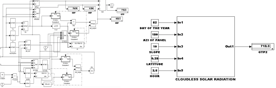
Fig. 3.Matlab/Simulink model of Cloudless Solar Radiation Structure

The detailed Simulink model done using the equations (1) – (17) is shown in the fig. 3. The inputs for modelling the solar radiation are (a) day of the year (b) Azimthal angle of the panel (c) Slope of the panel (d) Latitude of the place (e) Hour

Fig.4 PV Module Structure in Matlab

Parameter Value

Maximum Power 87W Voltage at MPP 17.4V Current at MPP 5.02A

Voc 21.7V

(6)

The detailed Simulink model of the PV module is done using the equations (18) – (25) is shown in the fig. 5. The inputs for modelling the solar module are the solar radiation obtained from the Simulink model shown in the fig. 4 and the specifications of the Solar panel listed in the table I

Fig. 5 Combined Structure Of Cloudless Solar Radiation and PV Module

The overall simulation model of the research work is shown n fig.5 By simulating the model Voltage – Current Curve and Power – Voltage curve of the PV module can be obtained.

Fig 6 I-V curves for various insolation levels

The Current – Voltage curves of the PV module is shown in the fig. 6 The I-V curves for the radiation obtained at a particular place is shown in the first figure and the I-V curve for the different radiation levels is shown in the next

(7)

The Power – Voltage curves of the PV module is shown in the fig. 7 The P-V curves for the radiation obtained at a particular place is shown in the first figure and the P-V curve for the different radiation levels is shown in the next

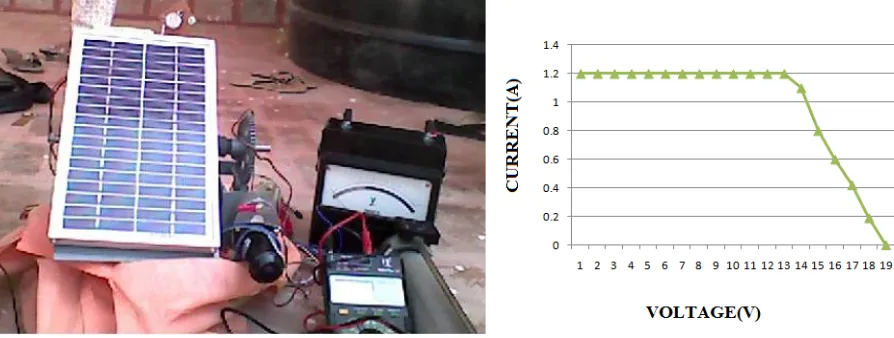
Fig. 8. Experimental Set up and V-I Characteristic Obtained from Experimental Setup

The hardware implementation of the research work is shown in the fig.8. The procedure to plot the I-V curve is to place the rheostat is different placed and note down the voltage and current readings. Then the readings are plotted using the graph in Microsoft excel. The I-V curves obtained is shown in fig.8

Fig. 9 Comparison between V-I curves obtained from Matlab/Simulink and Experimental Setup

As can be seen, Fig. 9 shows a very good agreement between the (voltage, current) points determined by the Simulink model and experimental data. The accuracy of the results could be improved if high precision apparatus were used and readings taken simultaneously by three different persons

X. CONCLUSION

(8)

REFERENCES

[1] DUSABE, D.—MUNDA, J. L.—JIMOH, A. A. : Modeling and Simulations of a Photovoltaic Module, Proceedings of the Fourth IASTED International Conference Power and Energy Systems (AsiaPES2008), Langkawi, Malaysia, April 2-4, 2008, pp. 327-333.

[2] De SOTO, W.—KLEIN, S. A.—BECKMAN, W. A. : Improvement and Validation of a Model for Photovoltaic Array Performance, Solar Energy 80 (2006), 78-88.

[3] MASTERS, G. M. : Renewable and Efficient Electric Power Systems, John Wiley & Sons, New Jersey, 2004.

[4] GRACE, W. : A Model of Diffuse Broadband Solar Irradiance for a Cloudless Sky, Australia meteorology magazine 55 (2006), 119-130. [5] MAXWELLL, E. L.—STOFFEL, T. L.—BIRD, R. E. : Measurement and Modelling Solar Irradiance on Vertical Surfaces [Online],

http://www.nrel.gov/docs/legosti/old/2525.pdf [Ac-cessed: 24/05/2008].

[6] T. Esram and P. L. Chapman, “Comparison of photovoltaic array maximum power point tracking techniques,” IEEE Trans. Energy Convers.,vol. 22, no. 2, pp. 439–449, Jun. 2007.

[7] E. Roman, R. Alonso, P. Ibanez, S. Elorduizapatarietxe, and D.Goitia,“Intelligent PV module for grid-connected PV systems,” IEEE Trans. Ind.Electron., vol. 53, no. 4, pp. 1066–1073, Jun. 2006.

[8] F. Salem, M. S. Adel Moteleb, and H. T. Dorrah, “An enhanced fuzzy- PI controller applied to the MPPT problem,” J. Sci. Eng., vol. 8, no. 2, pp. 147–153, 2005.F. Liu, S. Duan, F. Liu, B. Liu, and Y. Kang, “A variable step size INCMPPT method for PV systems,” IEEE Trans. Ind. Electron., vol. 55, no. 7,pp. 2622–2628, Jul. 2008.

[9] F. M. González-Longatt, “Model of photovoltaic module in Matlab,” in 2do congresoiberoamericano de estudiantes de ingenierıacute;aeléc- trica, electronicaycomputación, ii cibelec, pp. 1–5, 2005.

[10] N. Femia, D. Granozio, G. Petrone, G. Spagnuolo, and M. Vitelli, “Predictive & adaptive MPPT perturb and observe method,” IEEE Trans. Aerosp. Electron. Syst., vol. 43, no. 3, pp. 934–950, Jul. 2007.

[11] Gomathi B and Sivakami P, “An Incremental Conductance Algorithm based Solar Maximum Power Point Tracking System,” International Journal of Electrical Engineering, Volume 9, Number 1 (2016), pp. 15-24, Jan 2016