MM Algorithms for Variance Components Models.

ABSTRACT

HU, LIUYI. MM Algorithms for Variance Components Models. (Under the direction of Wenbin Lu and Hua Zhou.)

The classical linear regression model assumes independence among the observations. How-ever, in many real applications such as clustered data analysis and longitudinal data analysis, observations are correlated with each other and people are interested in estimating the variance from different sources. For example, in genetic analysis, people coming from the same family share common genetic information and researchers would like to know how much variation in the traits can be explained by the genetic effect. Despite the best efforts of generations of statisticians and numerical analysts, maximum likelihood estimation and restricted maximum likelihood estimation of variance component models remain numerically challenging. Building on the minorization-maximization (MM) principle, this thesis work presents novel iterative algorithms for variance components estimation as well as selection.

For the first part of the thesis, we develop MM algorithms in the linear mixed model frame-work where we assume the covariance structures are known. The proposed algorithm is trivial to implement and competitive on large data problems. The algorithm readily extends to more complicated problems such as linear mixed models, multivariate response models possibly with missing data, maximum a posteriori estimation and penalized estimation. We establish the global convergence of the MM algorithm to a KKT point and demonstrate, both numerically and theoretically, that it converges faster than the classical EM algorithm when the number of variance components is greater than two and all covariance matrices are positive definite.

©Copyright 2018 by Liuyi Hu

MM Algorithms for Variance Components Models

by Liuyi Hu

A dissertation submitted to the Graduate Faculty of North Carolina State University

in partial fulfillment of the requirements for the Degree of

Doctor of Philosophy

Statistics

Raleigh, North Carolina 2018

APPROVED BY:

Eric Chi Luo Xiao

Wenbin Lu

Co-chair of Advisory Committee

Hua Zhou

DEDICATION

BIOGRAPHY

ACKNOWLEDGEMENTS

I would like to thank my advisors, Dr. Hua Zhou and Dr. Wenbin Lu, for their patient guidance, knowledge and inspiational ideas. I would also like to thank Dr. Eric Chi and Dr. Luo Xiao for serving on my committee. Dr. Hua Zhou’s computing course inspired my interest in the statistical computing area and I am fortunate to have him as my co-advisor. Dr. Hua Zhou’s dedication, enthusiam and passion into research has inspired me a lot. And his attitude towards work has deeply influenced my life. I am also fortunate to have Dr. Wenbin Lu as my co-advisor after Dr. Hua Zhou moved to UCLA. Dr. Wenbin Lu is very smart and knowledgeable and has always been able to provide insightful guidance during our weekly meeting. They have helped me a lot not only in research but also in career development. I am blessed to have such nice advisors.

I am also very grateful to the faculty and staff at North Carolina State Univeristy. Even though Dr. Howard Bondell is no longer my committee member, I still want to thank him for the time and valuable feedback for this thesis work. I appreciate the research assistantship position that Dr. Eric Chi offered me. I appreciate his generous guidance, patience and valu-able mentorship. I would like to thank Terry Byron and Chris Waddell for their kind help on computer related problems. I also want to thank Alison McCoy for always willing to help me out.

TABLE OF CONTENTS

LIST OF TABLES . . . vii

LIST OF FIGURES . . . .viii

Chapter 1 Introduction . . . 1

1.1 Variance Components Model . . . 1

1.2 Optimization Techniques . . . 3

Chapter 2 Preliminaries . . . 6

2.1 The MM Principle . . . 6

2.2 Convex Matrix Functions . . . 7

2.3 Supporting Hyperplane Minorization . . . 8

2.4 Quadratic Minorization . . . 8

Chapter 3 MM Algorithms for Linear Mixed Model . . . 10

3.1 Introduction . . . 10

3.2 Univariate Response Model . . . 11

3.3 Numerical Experiments . . . 16

3.4 Global Convergence of the MM Algorithm . . . 17

3.5 MM versus EM . . . 26

3.6 Extensions . . . 30

3.6.1 Multivariate Response Model . . . 30

3.6.2 Multivariate Response Model with Missing Responses . . . 36

3.6.3 Linear Mixed Model (LMM) . . . 37

3.6.4 MAP Estimation . . . 40

3.6.5 Variable Selection . . . 41

3.7 A Numerical Example . . . 42

3.8 Discussion . . . 43

Chapter 4 MM Algorithms for Logistic Linear Mixed Model . . . 45

4.1 Introduction . . . 45

4.2 Algorithms for Estimation . . . 47

4.2.1 Model Formulation 1 . . . 47

4.2.2 Model Formulation 2 . . . 52

4.2.3 MM Algorithm for Maximizing the Penalized Approximated Likelihood . 55 4.2.4 Choice of Regularization Parameter . . . 56

4.3 Simulation Studies . . . 57

4.3.1 Random Effects ANOVA . . . 57

4.3.2 Genetic Example . . . 60

4.4 Real Data Analysis . . . 62

4.5 Discussion . . . 63

Appendix . . . 75

LIST OF TABLES

Table 3.1 Average iterations until convergence for MM, quasi-Newton accelerated MM (aMM), EM, and Fisher scoring (FS) for fitting a two-way ANOVA model with a=b= 5 levels of both factors. Standard errors are given in parentheses. 18 Table 3.2 Average run times (×10−3 _{seconds) of MM, quasi-Newton accelerated MM}

(aMM), EM, and Fisher scoring (FS) for fitting a two-way ANOVA model with a=b= 5 levels of both factors. Standard errors are given in parentheses. 19 Table 3.3 Rooted mean squared error (RMSE) of ˆσ2 _{using MM, quasi-Newton,}

acceler-ated MM (aMM), EM, and Fisher scoring (FS) for fitting a two-way ANOVA model with a = b = 5 levels of both factors. Standard errors are given in

parentheses. . . 20

Table 3.4 Rooted mean squared error (RMSE) of fixed effects and variance components in the genetic model. Standard errors are given in parentheses. . . 21

Table 3.5 Average performance of MM, quasi-Newton accelerated MM (aMM), EM, and Fisher scoring (FS) for fitting a genetic model. Standard errors are given in parentheses. . . 22

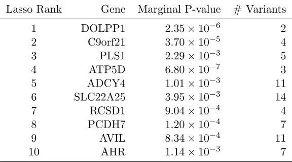
Table 3.6 Top 10 genes selected by the lasso penalized variance component model (3.18) in an association study of 200 genes and the complex traitheight. . . 43

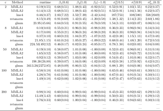
Table 4.1 Comparison of the MM algorithms with two different parameterizations (MMLA1 and MMLA2) and the glmer() function (with nAGQ=1) in thelme4 package, rstanarmpackage, andglmm package. Standard errors are given in parenthe-ses. Results forrstanarmandglmmwithc= 100,200 are not reported because the simulation takes more than 1 week. . . 59

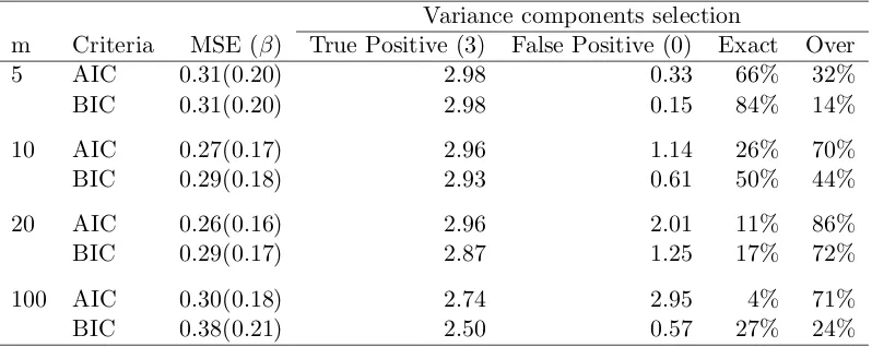
Table 4.2 Estimation and selection results for Setting 1. . . 61

Table 4.3 Estimation and selection results for Setting 2. . . 61

Table 4.4 Estimation and selection results for Setting 3. . . 62

Table 4.5 Estimation and selection results for Setting 4. . . 62

Table 4.6 Top 5 genes selected by (1) the lasso penalized variance component model (4.17) with AIC criterion (PLVC-AIC) and (2) SKAT in an association study of 200 genes and the binary traitsmoke. . . 64

LIST OF FIGURES

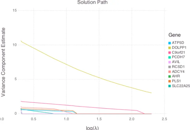
Figure 2.1 Log-likelihood surface of a 2-variance component model and the surrogate functions of EM and MM minorizing the objective function at point (σ₁2(t), σ₂2(t)) = (18.5,0.7). . . 9 Figure 3.1 Solution path of the lasso penalized variance component model (3.18) in an

association study of 200 genes and the complex traitheight. . . 44 Figure 4.1 Log-likelihood evaluation with top 5 genes selected by PLVC-AIC and SKAT

Chapter 1

Introduction

1.1

Variance Components Model

In statistics, linear regression model is an approach for modeling the linear relationship between the mean of the response variable and a set of explanatory variables (or predictors). Let us denote the set of observed response as a n×1 column vector y= (y1, . . . , yn)T and the set of explanatory variables as an×ppredictor matrixX, where each row ofX refers an observation and each column refers to a predictor. The classical linear regression model assumes yto be a realization of a random variable Y, which is normally distributed with

E(Y) =Xβand Cov(Y) =σ2I,

whereβis the unknown parameter. Thus the response variables are assumed to be independent of each other and to have equal variance. However, in many applications, reponses are correlated in a certain way. For example, a genetic study might try to answer what are the factors affecting people’s height. It is not reasonable to assume that people’s heights are independent of each other since people from the same family share common genes which might lead to similar heights. Also longitudinal studies observes a response variable repeated for each subject at different time points. The observations coming from the same subject are usually correlated with each other. Analysis that ignores the correlation structure will lead to invalid standard errors. Sometimes the observations are correlated via different structures and researchers want to study the variance of different structures. In this scenario, variance compomemts model comes into play.

The simplest form of variance components model assumes thatY ∼N(Xβ,Ω), where

Ω =

m

X

and the V1, . . . ,Vm arem fixed positive semidefinite matrices. The parameters of interest are

β and variance componentsσ2= (σ₁2, . . . , σ2_m)T.

For example, a genetic study wants to analyze the traits of n related individuals. It is assumed thatY ∼N(Xβ, σ₁2Φ+σ₂2I) where Φis the kinship coefficient matrix summarizing genetic similarity between individuals. The toal variability, having two variance components, is σ₁2+σ₂2. The heritability effect is the proportion of variation explained by genetic effects, that isσ2₁/(σ₁2+σ₂2).

Another example is the multilevel models where the data structure is hierarchical with sampled units nested in clusters that are themselves nested in other clusters. Suppose researchers want to study the students’ performance on GRE and they sample students from a sample of schools and a sample of departments under the school. Students in the same school and same department tend to be more alike than students in different schools or different departments. A multilevel model that takes into account the random effects of different levels has the form

yijk=xT_ijkβ+αi+γij +ijk,

where xijk is the vector of characteristics of students, {αi} are the random effects for schools and {γij} are the random effects for departments under each school. We assume that αi, γij andijkare independent with normal distributionsN(0, σ2α), N(0, σγ2) andN(0, σ2). The school level radom effects account for the variability among schools from unmeasured variables such as the quality of teachers. The department level random effects account for the deparment characteristics such as emphasis on math or verbals. The three variance components, σ2_α, σ_γ2 andσ2 can help us understand the intraclass correlation between scores of different students in the same department and same school.

An extention to the standard variance components models is to encompass non-normal response distributions. Just like the generalized linear models (GLM), the generalized variance components model assumes that E(Y) = µ, g(µ) = η where g(·) is some link function and

η∼N(Xβ,Ω), where

Ω =

m

X

i=1 σ_i2Vi.

For example, when the response is binary,g(·) can take the logic link functiong(x) = ln(x/(1− x)). When the response variables have counts as their possible values, we can use the log link g(x) = ln(x).

1.2

Optimization Techniques

In the above mentioned variance components model, the parameters of interest include coeffi-cientsβand the variance componentsσ2= (σ₁2, . . . , σ2_m)T. In statistical models, maximum like-lihood estimate (MLE) of parameters are widely used. However, in most applications, there are no explicit solutions to the original optimization problem. Therefore, we need iterative methods. Two commonly used iterative methods include Newton’s method and expectation maximiza-tion (EM) algorithm. Here we give an overview of these optimizamaximiza-tion methods. Throughout we reserve Greek letters for parameters and indicate the current iteration number by a superscript t.

Newton’s Method

The Newton’s method is built on maximizing the quadratic approximation of the original ob-jective function. Denote the obob-jective function asf(θ) and take second-order Taylor expansion at the current iterate θ(t), we have

f(θ)≈f(θ(t)) +∇f(θ(t))T(θ−θ(t)) +1 2(θ−θ

(t)₎T_∇2_f(θ(t)_)(θ−θ(t)₎

where∇f(θ(t)) is the gradient of thef(θ) evaluated at current iterateθ(t)and∇2_f(θ(t)_{) is the} Hessian matrix of f(θ) evaluated at current iterate θ(t). To maximize the quadratic function, we set its gradient to zero, which yields the following update

θ(t+1) =θ(t)−n∇2f(θ(t))

o−1

∇f(θ(t)).

The Newton’s method is a second-order algorithm and can converge very fast. However, it has several drawbacks. The first is that in the vanilla version each iteration involves the evaluation and inversion of the Hessian matrix, which can be very computational expensive, especially when the parameter space is high dimensional. The second is that Newton’s method can not guarantee ascent property when the Hessian matrix is not negative definite. The third is that when the Hessian matrix is close to singular matrix, the inverted Hessian can be numerically unstable and the solution may diverge. There are several remedies to address these issues. Most of them involve approximating−∇2_f(θ(t)_{) by a positive definite matrix, which leads to variants} of Newton’s method.

The general form of Newton’s method is

wheresis the step size andM(θ(t)) is some approximation of−∇2_f(θ(t)_{). When M(θ}(t)_{) =I,} (1.1) is the same as the gradient descent method. The gradient descent method does not use the second order information, so it converges at a linear rate instead of quadratic rate. When M(θ(t)) = En−∇2_f(θ(t)₎o_{, (1.1) gives the Fisher’s scoring method. The Fisher’s} informa-tion matrix is positive semi-definite under exchangeability of expectainforma-tion and differentiainforma-tion, however, it could be hard to derive and computationally expensive to evaulate.

EM Algorithm

The EM algorithm was first introduced by Dempster et al. (1977) and it is widely used in models that involve observed dataX, unobserved latent variables Z and a vector of unknown parametersθ. The MLE ofθ is the one that maximizes the marginal likelihood of the observed data

f(X |θ) =

Z

p(X,Z|θ)dZ

wherep(X,Z|θ) is the density function of the complete data. However the marginal likelihood is often intractable especially whenZ involves high-dimensional data. The EM algorithm deals with the problem by working with the complete data model. It involves two steps:

- Expectation step (E step): Calculate the conditional expectation of the log-likelihood function of the complete data under the current estimate of the parameterθ(t)

Q(θ |θ(t)) = E

Z|X,θ(t){lnL(θ;X,Z)} whereL(θ;X,Z) =p(X,Z |θ).

- Maximization step (M step): Maximize Q(θ |θ(t))

θ(t+1) = arg max

θ Q(θ|θ

(t)_).

By the information inequality, we have

Q(θ|θ(t))−lnf(X |θ)

= E

Z|X,θ(t){lnL(θ;X,Z)} −lnf(X |θ)

= E

lnL(θ;X,Z) f(X |θ) |X,θ

(t)

≤ E

(

lnL(θ

(t)_;X,Z) f(X |θ(t)) |X,θ

(t)

)

which leads to the following inequality

lnf(X |θ)≥Q(θ|θ(t))−Q(θ(t)|θ(t)) + lnf(X |θ(t)) for all θ in the parameter space. Combining with the maximization step, we have

lnf(X |θ(t+1)) ≥ Q(θ(t+1) |θ(t))−Q(θ(t)|θ(t)) + lnf(X |θ(t)) ≥ lnf(X |θ(t)).

Chapter 2

Preliminaries

2.1

The MM Principle

The MM principle for maximizing an objective function f(θ) involves minorizing the objective function f(θ) by a surrogate function g(θ | θ(t)) around the current iterate θ(t) of a search (Lange et al., 2000). Minorization is defined by the two conditions

f(θ(t)) = g(θ(t) |θ(t)) (2.1)

f(θ) ≥ g(θ |θ(t)), θ6=θ(t).

In other words, the surface θ 7→ g(θ | θ(t)) lies below the surface θ 7→ f(θ) and is tangent to it at the point θ = θ(t). Construction of the minorizing function g(θ | θ(t)) constitutes the first M of the MM algorithm. The second M of the algorithm maximizes the surrogate g(θ|θ(t)) rather thanf(θ). The pointθ(t+1)maximizingg(θ|θ(t)) satisfies the ascent property f(θ(t+1))≥f(θ(t)). This fact follows from the inequalities

f(θ(t+1)) ≥ g(θ(t+1) |θ(t)) ≥ g(θ(t)|θ(t)) = f(θ(t)), (2.2) reflecting the definition ofθ(t+1)and the tangency and domination conditions (2.1). The ascent property makes the MM algorithm remarkably stable. The validity of the descent property depends only on increasing g(θ | θ(t)), not on maximizing g(θ | θ(t)). With obvious changes, the MM algorithm also applies to minimization rather than to maximization. To minimize a function f(θ), we majorize it by a surrogate function g(θ | θ(t)) and minimize g(θ | θ(t)) to produce the next iterate θ(t+1). The acronym should not be confused with the maximization-maximization algorithm in the variational Bayes context (Jeon, 2012).

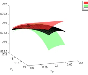
and Groenen, 2005), ranking of sports teams (Hunter, 2004), variable selection (Hunter and Li, 2005), optimal experiment design (Yu, 2010), multivariate statistics (Zhou and Lange, 2010), geometric programming (Lange and Zhou, 2014), and many other areas (Lange, 2016). The celebrated EM principle (Dempster et al., 1977) is a special case of the MM principle. The Q function produced in the E step of an EM algorithm minorizes the log-likelihood up to an irrelevant constant. Thus, both EM and MM share the same advantages: simplicity, stability, graceful adaptation to constraints, and the tendency to avoid large matrix inversion. The more general MM perspective frees algorithm derivation from the missing data straitjacket and invites wider applications (Wu and Lange, 2010). Figure 2.1 shows the minorization functions of EM and MM for a variance components model withm= 2 variance components.

EM and MM algorithms often exhibit slow convergence. Fortunately, this defect can be reme-died by off-the-shelf acceleration techniques for fixed point iterations. The recently developed squared iterative method (SQUAREM) (Varadhan and Roland, 2008) and the quasi-Newton acceleration method (Zhou et al., 2011) are particularly attractive, given their simplicity and minimal memory and computational costs. Our numerical experiments feature the unadorned MM algorithm and the quasi-Newton accelerated MM (aMM) algorithm based on one secant pair. Using more secant pairs is likely to further improve performance.

2.2

Convex Matrix Functions

For symmetric matrices we write A B when B −A is positive semidefinite and A ≺B if

B−A is positive definite. A matrix-valued functionf is said to be (matrix) convex if f{λA+ (1−λ)B} λf(A) + (1−λ)f(B)

for all A,B, and λ∈[0,1]. Our derivation of the MM variance components algorithm hinges on the convexity of the two functions mentioned in the next lemma.

Lemma 1. (a) The matrix fractional function f(A,B) = ATB−1A is jointly convex in the

m×n matrix A and them×m positive definite matrix B. (b) The log determinant function

f(B) = ln detB is concave on the set of positive definite matrices.

Proof. The matrix fractional function is matrix convex because its epigraph

{(A,B,C) :B0,ATB−1AC} =

(

(A,B,C) :B0, B A

AT C

!

0

)

the concavity of the log determinant, see Boyd and Vandenberghe (2004, p74).

2.3

Supporting Hyperplane Minorization

Iff(θ) is convex and differentiable, then the supporting hyperplane

g(θ) =f(θ(t)) +∇f(θ(t))T(θ−θ(t)) (2.3) is a minorization function off(θ) at θ(t) (Hunter and Lange, 2004b).

Since the negative log determinant function f(B) = −log detB is convex on the set of positive definite matrices (Boyd and Vandenberghe, 2004) and the supporting hyperplane of f(B) is

g(B) = f(B(t)) +∇f(B(t))T(B−B(t)) = −log detB(t)−tr

B(t)

−1

B−B(t)

,

the supporting hyperplane minorization described above yields the following inequality

−log detB≥ −log detB(t)−tr

B(t)−1B−B(t)

. (2.4)

2.4

Quadratic Minorization

If a convex function f(θ) is twice differentiable and there exists a matrix M such thatM ∇2_{f(θ) for allθ, then}

g(θ) =f(θ(t)) +∇f(θ(t))T(θ−θ(t)) +1 2(θ−θ

(t)₎T_M(θ−θ(t)_{) (2.5)}

0.6 0.65

0.7

σ 2 0.75 0.8

19 18.5 18

σ 1 -520.5

-521

-521.5

-522

-522.5 -520

17.5

logL EM MM

Chapter 3

MM Algorithms for Linear Mixed

Model

3.1

Introduction

Variance components and linear mixed models are among the most potent tools in a statistician’s toolbox. They are essential topics in graduate-level linear model courses and the subject of many current papers and research monographs (Rao and Kleffe, 1988; Searle et al., 1992; Rao, 1997; Khuri et al., 1998; Demidenko, 2013). Their applications in agriculture, biology, economics, genetics, epidemiology, and medicine are too numerous to cover here in detail. The recommended books (Verbeke and Molenberghs, 2000; Weiss, 2005; Fitzmaurice et al., 2011) stress longitudinal data analysis.

Given an observed n×1 response vector y and n×p predictor matrix X, the simplest variance components model postulates thatY ∼N(Xβ,Ω), where

Ω =

m

X

i=1 σ_i2Vi,

and theV1, . . . ,Vmaremfixed positive semidefinite matrices. The parameters of the model can be divided into mean effects (β1, . . . , βp) and variance components (σ₁2, . . . , σ2_m), summarized by vectors β and σ2_{. Throughout we assume Ωis positive definite. The extension to singular}

Ωwill not be pursued here. Estimation revolves around the log-likelihood function

L(β,σ2) = −1

2ln detΩ− 1

2(y−Xβ)

T_Ω−1_{(y−Xβ). (3.1)}

1977) are the most popular. REML first projects y to the null space of X and then estimates variance components based on the projected responses. If the columns of the matrix B span the null space of XT_{, then REML estimates the σ}2

i by maximizing the log-likelihood of the redefined response vector BTY, which is normally distributed with mean 0 and covariance

BTΩB =Pm

i=1σ2iBTViB.

There exists a large literature on iterative algorithms for finding MLE and REML (Laird and Ware, 1982; Lindstrom and Bates, 1988, 1990; Harville and Callanan, 1990; Callanan and Harville, 1991; Bates and Pinheiro, 1998; Schafer and Yucel, 2002). Fitting variance components models remains a challenge in models with a large sample size nor a large number of variance components m. Newton’s method (Lindstrom and Bates, 1988) converges quickly but is nu-merically unstable owing to the non-concavity of the log-likelihood. Fisher’s scoring algorithm replaces the observed information matrix in Newton’s method by the expected information ma-trix and yields an ascent algorithm when safeguarded by step halving. However the calculation and inversion of expected information matrices cost O(mn3) +O(m3) flops for unstructured

Vi and quickly become impractical when either norm is large. The expectation-maximization (EM) algorithm initiated by Dempster et al. is a third alternative (Dempster et al., 1977; Laird and Ware, 1982; Laird et al., 1987; Lindstrom and Bates, 1988; Bates and Pinheiro, 1998). Compared to Newton’s method, the EM algorithm is easy to implement and numerically sta-ble, but painfully slow to converge. In practice, a strategy of priming Newton’s method by a few EM steps leverages the stability of EM and the faster convergence of second-order methods. Quasi-Newton methods dispense with explicit calculation of the observed information while achieving a superlinear rate of convergence.

In this chapter we derive a minorization-maximization (MM) algorithm for finding the MLE and REML estimates of variance components. We prove global convergence of the MM algorithm to a Karush-Kuhn-Tucker (KKT) point and explain why MM generally converges faster than EM for models with more than two variance components. We also sketch extensions of the MM algorithm to the multivariate response model with possibly missing responses, the linear mixed model (LMM), maximum a posteriori (MAP) estimation and penalized estimation. The numerical efficiency of the MM algorithm is illustrated through simulated data sets and a genomic example with more than 200 variance components.

3.2

Univariate Response Model

problem with solution

β(t+1) = (XTΩ−(t)X)−1XTΩ−(t)y, (3.2) where Ω−(t) represents the inverse of Ω(t) =Pm

i=1σ 2(t)

i Vi. Updatingσ2 given β(t) depends on two minorizations. If we assume that all of theVi are positive definite, then the joint convexity of the map (X,Y)7→XTY−1X for positive definite Y implies that

Ω(t)Ω−1Ω(t) = m

X

i=1

σ_i2(t)Vi

! _m

X

i=1 σ2_iVi

!−1 _m

X

i=1

σ2(t)_i Vi

!

= m

X

i=1

σ_i2(t)

P jσ 2(t) j P jσ 2(t) j σ2(t)_i

σ_i2(t)Vi

!

· m

X

i=1

σ_i2(t)

P jσ 2(t) j P jσ 2(t) j σ2(t)_i

σ_i2Vi

!−1

· m

X

i=1

σ_i2(t)

P jσ 2(t) j P jσ 2(t) j σ_i2(t)

σ2(t)_i Vi

!

m

X

i=1

σ_i2(t)

P jσ 2(t) j P jσ 2(t) j σ_i2(t)

σ_i2(t)Vi

! P

jσ 2(t) j σ_i2(t)

σ_i2Vi

!−1 P

jσ 2(t) j σ2(t)_i

σ_i2(t)Vi

!

= m

X

i=1 σ4(t)_i

σ_i2 ViV −1 i Vi

= m

X

i=1 σ4(t)_i

σ_i2 Vi.

When one or more of the Vi are rank deficient, we replace eachVi by Vi, =Vi+I for >0 small and letΩ(t) =P_iσ_i2(t)Vi,. Sending to 0 in the just proved majorization

Ω(t) Ω−1 Ω(t) m

X

i=1 σ_i4(t)

σ_i2 Vi, gives the desired majorization

Ω(t)Ω−1Ω(t) m

X

i=1 σ4(t)_i

σ2 i

Vi

in the general case. Negating both sides leads to the minorization

−(y−Xβ)TΩ−1(y−Xβ) −(y−Xβ)TΩ−(t)

m

X

i=1 σ4(t)_i

σ2_i Vi

!

that effectively separates the variance components σ₁2, . . . , σ_m2 in the quadratic term of the log-likelihood (3.1).

The convexity of the function A 7→ −log detA is equivalent to the supporting hyperplane minorization

−ln detΩ ≥ −ln detΩ(t)−tr{Ω−(t)(Ω−Ω(t))} (3.4)

that separates σ2₁, . . . , σ_m2 in the log determinant term of the log-likelihood (3.1). Combination of the minorizations (3.3) and (3.4) gives the overall minorization

g(σ2 |σ2(t)) = −1

2tr(Ω

−(t)_Ω)−1

2(y−Xβ

(t)₎T_Ω−(t) m

X

i=1 σ4(t)_i

σ_i2 Vi

!

Ω−(t)(y−Xβ(t)) +c(t) (3.5)

= m X i=1 ( −σ 2 i 2 tr(Ω

−(t)

Vi)−1 2

σ4(t)_i

σ_i2 (y−Xβ

(t)₎T_Ω−(t)

ViΩ−(t)(y−Xβ(t))

)

+c(t),

wherec(t) is an irrelevant constant. Maximization ofg(σ2 |σ2(t)) with respect to σ_i2 yields the lovely multiplicative update

σ2(t+1)_i = σ_i2(t)

s

(y−Xβ(t))T_Ω−(t)_V

iΩ−(t)(y−Xβ(t)) tr(Ω−(t)Vi)

, i= 1, . . . , m. (3.6)

To preserve the uniqueness and continuity of the algorithm map, we must take σ_i2(t+1) = 0 whenever σ_i2(t)= 0. As a sanity check on our derivation, consider the partial derivative

∂ ∂σ2

i

L(β,σ2) = −1 2tr(Ω

−1

Vi) +1

2(y−Xβ) T_Ω−1

ViΩ−1(y−Xβ). (3.7)

Given σ_i2(t)>0, it is clear from the update formula (3.6) that σ2(t+1)_i < σ_i2(t) when _∂σ∂2

i

L <0. Conversely σ_i2(t+1) > σ_i2(t) when _∂σ∂2

i

L > 0. Algorithm 1 summarizes the MM algorithm for MLE of the univariate response model (3.1).

The update formula (3.6) assumes that the numerator under the square root sign is nonneg-ative and the denominator is positive. The numerator requirement is a consequence of the posi-tive semidefiniteness ofVi. The denominator requirement can be verified through the Hadamard (elementwise) product representation tr(Ω−(t)Vi) =1T(Ω−(t)Vi)1. The following lemma of Schur (1911) is crucial. We give a self-contained probabilistic proof.

Input :y,X,V1, . . . ,Vm

Output: MLE ˆβ, ˆσ₁2, . . . ,σˆ_m2

1 Initialize σ_i(0) >0,i= 1, . . . , m; 2 repeat

3 Ω(t)←Pm_i=1σ_i2(t)V_i ;

4 β(t) ←arg min_β(y−Xβ)TΩ−(t)(y−Xβ)

σ2(t+1)_i ←σ_i2(t)

r

(y−Xβ(t))T_Ω−(t)_ViΩ−(t)_(y−Xβ(t)₎

tr(Ω−(t)Vi)

, i= 1, . . . , m;

5 until objective value converges;

Algorithm 1:MM algorithm for MLE of the variance components of model (3.1).

Proof. Let X = (X1, . . . , Xn)T be a random normal vector with mean 0 and positive definite covariance matrix A. Let Y = (Y1, . . . , Yn)T be a random normal vector independent of X with mean 0 and positive semidefinite covariance matrix B having positive diagonal entries. Then Z = X Y has covariances E(ZiZj) = E(XiYiXjYj) = E(XiXj)E(YiYj) = aijbij. It follows that Cov(Z) = AB. To show AB is positive definite, suppose on the contrary thatvT(AB)v = Var(vTZ) = 0 for some v 6=0. Then

0 = Var(vTZ) = E X i

viXiYi

2

= E

( X

i

viXiYi

2

|Y

)

= E

(vY)TA(vY)

implies vY =0 with probability 1. Since v 6=0,Yi = 0 with probability 1 for somei. This contradicts the assumptionbii= Var(Yi)>0 for alli.

We can now obtain the following characterization of the MM iterates.

Proposition 1. Assume Vi has strictly positive diagonal entries. Thentr(Ω−(t)Vi)>0for all t. Furthermore if σ2(0)_i >0 and Ω−(t)(y−Xβ(t)) ∈/ null(Vi) for all t, then σ_i2(t)>0 for all t. When Vi is positive definite, σi2(t)>0 holds if and only if y6=Xβ(t).

Proof. The first claim follows easily from Schur’s lemma. The second claim follows by induction. The third claim follows from the observation that null(Vi) ={0}.

Univariate Response: Two Variance Components

Input :y,X,V1,V2

Output: MLE ˆβ, ˆσ₁2,σˆ₂2

1 Simultaneous congruence decomposition: (D,U)←(V1,V2) ; 2 Transform data: ˜y←UTy, ˜X ←UTX ;

3 Initialize σ₁(0), σ(0)₁ >0 ; 4 repeat

5 w_i(t)←(σ₁2(t)di+σ₂2(t))−1, i= 1, . . . , n ; 6 β(t) ←arg min_β Pn_i=1w_i(t)(˜yi−x˜T_i β)2

σ2(t+1)₁ ←σ₁2(t)

s

( ˜y−_X˜_β(t)₎T_(σ2(t)

1 D+σ 2(t)

2 I)−1D(σ 2(t) 1 D+σ

2(t)

2 I)−1( ˜y−X˜β (t)

) trn(σ₁2(t)D+σ₂2(t)I)−1_Do ;

7 σ2(t+1)₂ ←σ₂2(t) s

( ˜y−_X˜_β(t)

)T_(σ2(t)

1 D+σ 2(t)

2 I)−2( ˜y−X˜β (t)

) tr

n

(σ₁2(t)D+σ₂2(t)I)−1o ;

8 until objective value converges;

Algorithm 2: Simplified MM algorithm for MLE of model (3.1) with m = 2 variance components and Ω=σ₁2V1+σ22V2.

The major computational cost of Algorithm 1 is inversion of the covariance matrix Ω(t) at each iteration. The special case of m= 2 variance components deserves attention as repeated matrix inversion can be avoided by invoking the simultaneous congruence decomposition for two symmetric matrices, one of which is positive definite (Rao, 1973; Horn and Johnson, 1985). This decomposition is also called the generalized eigenvalue decomposition (Golub and Van Loan, 1996; Boyd and Vandenberghe, 2004). If one assumes Ω = σ₁2V1+σ22V2 and lets (V1,V2) 7→ (D,U) be the decomposition with U nonsingular, UTV1U = D diagonal, and UTV2U = I, then

Ω(t) = U−T(σ₁2(t)D+σ2(t)₂ In)U−1 Ω−(t) = U(σ2(t)₁ D+σ₂2(t)In)−1UT

det(Ω(t)) = det(σ₁2(t)D+σ2(t)₂ In) det(U−TU−1) (3.8) = det(σ₁2(t)D+σ2(t)₂ In) det(V2).

w(t)_i = (σ2(t)₁ di+σ2(t)2 )−1. Algorithm 2 summarizes the simplified MM algorithm for two variance components.

3.3

Numerical Experiments

This section compares the numerical performance of MM, quasi-Newton accelerated MM, EM, and Fisher scoring on simulated data from a two-way ANOVA random effects model and a genetic model. For ease of comparison, all algorithm runs start from σ2(0) =1 and terminate when the relative change (L(t+1)−L(t))/(|L(t)_{|+ 1) in the log-likelihood is less than 10}−6_{. In} order to respect nonnegativity constraint, quasi-Newton acceleration is performed on positive square root ofσ2_i.

Two-way ANOVA: We simulated data from a two-way ANOVA random effects model

yijk =µ+αi+βj+ (αβ)ij+ijk,1≤i≤a,1≤j≤b,1≤k≤k,

whereαi∼N(0, σ21),βj ∼N(0, σ22), (αβ)ij ∼N(0, σ32), andijk∼N(0, σe2) are jointly indepen-dent. Here iindexes levels in factor 1, j indexes levels in factor 2, and k indexes observations in the (i, j)-combination. This corresponds to m = 4 variance components. In the simulation, we set σ₂2 =σ2₃ =σ_e2 and varied the ratio σ₁2/σ2_e; the numbers of levels aand b in factor 1 and factor 2, respectively; and the number of observations c in each combination of factor levels. For each simulation scenario, we simulated 50 replicates. The sample size wasn=abcfor each replicate.

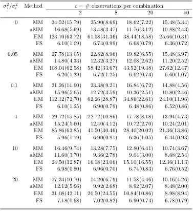
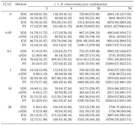
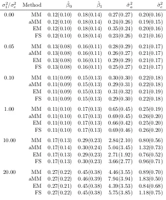
Tables 3.1 and 3.2 show the average number of iterations and the average runtimes when there are a=b= 5 levels of each factor. Based on these results and further results not shown for other combinations of aand b, we draw the following conclusions. Fisher scoring takes the fewest iterations. The MM algorithm always takes fewer iterations than the EM algorithm. Accelerated MM further improves the convergence rate of MM. The faster rate of convergence of Fisher scoring is outweighed by the extra cost of evaluating and inverting the covariance matrix. When the sample size n =abc is large, Fisher scoring takes much longer than either EM or MM.

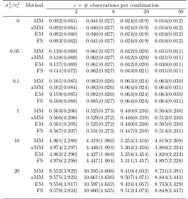
Table 3.3 summarizes the the rooted mean squared error (RMSE) of the variance components

σ2= (σ₁2, σ2₂, σ₃2, σ_e2). For each replicate, RMSE is calculated as

v u u t

1 4

4

X

j=1 (ˆσ2

j −σ2j)2. (3.9)

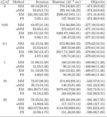
Genetic model:We simulated a quantitative traityfrom a genetic model with two variance components and covariance matrix Ω= σ_a2Φb +σ2_eI, where Φb is a full-rank empirical kinship

matrix estimated from the genome-wide measurements of 212 individuals using Option 29 of the Mendel software (Lange et al., 2013). Table 3.4 summarizes the RMSE of each parameter: the intercept β0, the slope for gender β1, and two variance components σ2_a and σ2_e. Table 3.5 summarizes the iteration number, runtime and objective value for different algorithms. In this example, Fisher scoring excels at smallerσ2_a/σ2_e ratios, while accelerated MM is fastest at larger σ_a2/σ2_e ratios.

In summary, the MM algorithm appears competitive even in small-scale examples. Modern applications often involve a large number of variance components. In this setting, the EM algorithm suffers from slow convergence and Fisher scoring from an extremely high cost per iteration. Our genomic example in Section 3.7 reinforces this point.

3.4

Global Convergence of the MM Algorithm

The KKT necessary conditions for a local maximum σ2 = (σ2₁, . . . , σ_m2) of the log-likelihood (3.1) require each component of the score vector to satisfy

∂ ∂σ_i2L(σ

2_{) ∈}







{0} σ2 i >0 (−∞,0] σ2_i = 0.

In this section we establish the global convergence of Algorithm 1 to a KKT point. To reduce the notational burden, we assume that X is null and omit estimation of fixed effects β. The analysis easily extends to the MLE case. Our convergence analysis relies on characterizing the properties of the objective function L(σ2) and the MM algorithmic mapping σ2 7→ M(σ2) defined by equation (3.6). Special attention must be paid to the boundary values σ_i2 = 0. We prove convergences for two cases, which cover most applications. The genetic model in Section 3.2 satisfies Assumption 1, while the two-way ANOVA model satisfies Assumption 2.

Assumption 1. All Vi are positive definite.

Assumption 2. V1 is positive definite, each Vi is nontrivial, H =span{V2, . . . ,Vm} has

di-mension q < n, andy∈ H/ .

The key condition y ∈/ span{V2, . . . ,Vm} in the second case is critical for the existence of an MLE or REML (Demidenko and Massam, 1999; Grzadziel and Michalski, 2014). We will derive a sequence of lemmas en route to the global convergence result declared in Theorem 1.

Table 3.1: Average iterations until convergence for MM, quasi-Newton accelerated MM (aMM), EM, and Fisher scoring (FS) for fitting a two-way ANOVA model witha=b= 5 levels of both factors. Standard errors are given in parentheses.

σ2

1/σ2e Method c= # observations per combination

2 8 20 50

Table 3.2: Average run times (×10−3 seconds) of MM, quasi-Newton accelerated MM (aMM), EM, and Fisher scoring (FS) for fitting a two-way ANOVA model witha=b= 5 levels of both factors. Standard errors are given in parentheses.

σ2₁/σ2_e Method c = # observations per combination

2 8 20 50

Table 3.3: Rooted mean squared error (RMSE) of ˆσ2 _{using MM, quasi-Newton, accelerated} MM (aMM), EM, and Fisher scoring (FS) for fitting a two-way ANOVA model with a=b= 5 levels of both factors. Standard errors are given in parentheses.

σ2₁/σ2_e Method c = # observations per combination

2 8 20 50

Table 3.4: Rooted mean squared error (RMSE) of fixed effects and variance components in the genetic model. Standard errors are given in parentheses.

Table 3.5: Average performance of MM, quasi-Newton accelerated MM (aMM), EM, and Fisher scoring (FS) for fitting a genetic model. Standard errors are given in parentheses.

Proof. Let us first prove the assertion when all of the covariance matricesViare positive definite. If we setr=kσ2k1 andαi=r−1σ2i for each i, then the log-likelihood satisfies

L(σ2) = −n 2lnr−

1 2ln det

Xm

i=1 αiVi

− 1 2ry T m X i=1 αiVi

−1

y.

The functions ln detPm

i=1αiVi

andyTPm

i=1αiVi

−1

yof αare defined and continuous on the unit simplex and hence bounded there. The dominant term −n

2lnr of the loglikelihood tends to −∞asr tends to∞.

To prove the assertion under Assumption 2, consider first the case V1 =In. Setting αi = σ_i2/σ2₁ fori= 2, . . . , m reduces the loglikelihood to

L(σ₁2,α) = −n 2 lnσ

2 1 −

1 2ln det

In+ m

X

i=2 αiVi

− 1 2σ₁2y

T_I n+

m

X

i=2 αiVi

−1

y. (3.10)

The middle term on the right satisfies

−1 2ln det

In+ m

X

i=2 αiVi

≤ 0

because det (In+Pm_i=2αiVi) ≥ detIn = 1. Now let U = (Uq,Un−q) be an n×n orthogonal matrix whose left columns Uq span Hand whose right columnsUn−q span H⊥. The identity

UTIn+ m

X

i=2 αiVi

U = Iq+

Pm

i=2αiUqTViUq 0

0 In−q

!

follows from the orthogonality relationsU_n−qT Vi = Un−qT Uq = 0(n−q)×n. This in turn implies

In+ m

X

i=2 αiVi

−1

= U (Iq+

Pm

i=2αiUqTViUq)−1 0

0 In−q

!

UT

U 0 0 0 In−q

!

UT

= Un−qUn−qT .

Therefore the quadratic term in equation (3.10) is bounded below by the positive constant

yTIn+ m

X

i=2 αiVi

−1

Here the assumptiony∈ H/ guarantees the projection propertyPH⊥y6=0.

Next we show that the loglikelihood tends to −∞ when σ₁2 tends to 0 or ∞ or whenkαk2 tends to ∞. The second of the two inequalities

L(σ₀2,α) ≤ −n 2 lnσ

2 1 −

1 2ln det

In+ m

X

i=2 αiVi

− 1

2σ₁2kPH⊥yk 2

≤ −n 2 lnσ

2 1 −

1

2σ₁2kPH⊥yk 2

renders the claim aboutσ2

1 obvious. To prove the claim aboutα, we make the worst case choice σ_i2 =k_PH⊥yk2 in the first inequality. It follows that

L(σ₀2,α) ≤ −1 2ln det

In+ m

X

i=2 αiVi

−n

2lnkPH⊥yk 2₋n

2. Ifαj tends to ∞, then the inequality

−1 2ln det

In+ m

X

i=2 αiVi

≤ −1 2ln det

In+αjVj

= −1 2

n

X

k=1

ln(1 +αjλjk)

holds, where the λjk are the eigenvalues of Vj. At least one of these eigenvalues is positive because Vj is nontrivial. It follows thatL(σ02,α) tends to −∞ in this case as well.

For the general case where V1 is non-singular but not necessarily In, let V11/2 be the sym-metric square root ofV1 and write

V1+ m

X

i=2

σ_i2Vi=V11/2 I+ m

X

i=2

σ2_iV₁−1/2ViV −1/2 1

!

V₁1/2.

The above arguments still apply since each V₁−1/2ViV₁−1/2 is nontrivial and y belongs to the span{V2, . . . ,Vm}=S if and only if V

−1/2

1 y belongs toV −1/2 1 SV

−1/2 1 .

Lemma 4. The iterates possess the ascent property L(M(σ2(t))) ≥ L(σ2(t)). Furthermore, whenL(M(σ2∗)) =L(σ2∗),σ2∗ fulfills the fixed point conditionM(σ2∗) =σ2∗, and each component

satisfies either (i) σ2_∗i = 0 or (ii)σ2_∗i >0 and _∂σ∂2

i

L(σ2∗) = 0.

Proof. The ascent property is built into any MM algorithm. Suppose L(M(σ2∗)) =L(σ2∗) at a point σ2

∗∈Rm+. Then equality must hold in the string of inequalities (2.2). It follows that g(M(σ2∗)|σ2∗) = g(σ2∗ |σ2∗).

henceM(σ2_∗) =σ2_∗. Ifσ_∗i2 >0, the stationarity condition ∂

∂σ_i2L(σ 2 ∗) =

∂ ∂σ2_ig(σ

2

∗|σ2∗) = 0

applies. The equivalence of the two displayed partial derivatives is a consequence of the fact that the difference f(σ2_)−g(σ2 _|σ2

∗) achieves its minimum of 0 atσ2=σ2∗.

Lemma 5. The distance between successive iterates kσ2(t+1)−σ2(t)k2 converges to 0.

Proof. Suppose on the contrary that kσ2(t+1)−σ2(t)k2 does not converge to 0. Then one can extract a subsequence{t_k}k≥1 such that

kσ2(tk+1)_−σ2(tk)_k

2 ≥ >0 (3.11)

for all k. Let C0 be the compact super-level set {σ2 : L(σ2) ≥ L(σ2(0))}. Since the sequence {σ2(tk)_}

k≥1 is confined toC0, one can pass to a subsequence if necessary and assume thatσ2(tk) converges to a limitσ2∗ and thatσ2(tk+1) converges to a limitσ2∗∗. Taking limits in the relation

σ2(tk+1) _{= M(σ}2(tk)_{) and invoking the continuity M(σ}2_{) imply that σ}2

∗∗ = M(σ2∗). Because the sequenceL(σ2(tk)_{) is monotonically increasing in kand bounded above on C}

0, it converges to a limit L∗. Hence, the continuity ofL(σ2) implies

L(σ2_∗) = lim k L(σ

2(tk)_{) = L∗ = lim}

k L(σ

2(tk+1)_{) = L(σ}2

∗∗) = L(M(σ2∗)). Lemma 4 therefore givesσ2∗∗=M(σ2∗) =σ2∗, contradicting the boundkσ2∗−σ2∗∗k2≥entailed by inequality (3.11).

Theorem 1. The MM sequence {σ2(t)}t≥0 has at least one limit point. Every limit point is a

fixed point of M(σ2_{). If the set of fixed points is discrete, then the MM sequence converges to}

one of them. Finally, when the iterates converge, their limit is a KKT point.

Proof. The sequence{σ2(t)}t≥0is contained in the super-level compact setC0defined in Lemma 5 and therefore admits a convergent subsequenceσ2(tk) _{with limitσ}2(∞)_{. As argued in Lemma}

5,L(σ2(∞)) =L(M(σ2(∞))). Lemma 4 now implies thatσ2(∞)is a fixed point of the algorithm mapM(σ2).

According to Ostrowski’s theorem (Lange, 2010, Proposition 8.2.1), the set of limit points of a bounded sequence{σ2(t)_}

has a non-positive partial derivative. Suppose on the contraryσ2(∞)_i = 0 and _∂σ∂2

i

L(σ2(∞))>0. By continuity _∂σ∂2

i

L(σ2(t)) > 0 for all large t. Therefore, σ2(t+1)_i > σ2(t)_i for all large t by the observation made after equation (3.7). This behavior is inconsistent with the assumption that σ_i2(t)→0.

3.5

MM versus EM

Examination of Tables 3.2 and 3.5 suggests that the MM algorithm usually converges faster than the EM algorithm. We now provide theoretical justification for this observation. Again for notational convenience, we consider the REML case whereX is null. Since the EM principle is just a special instance of the MM principle, we can compare their convergence properties in a unified framework. Consider an MM mapM(θ) for maximizing the objective functionf(θ) via the surrogate functiong(θ|θ(t)). Close to the optimal pointθ∞,

θ(t+1)−θ∞ ≈ dM(θ∞)(θ(t)−θ∞),

where dM(θ∞) is the differential of the mapping M at the optimal point θ∞ of f(θ). Hence, the local convergence rate of the sequence θ(t+1) =M(θ(t)) coincides with the spectral radius of dM(θ∞). Familiar calculations (McLachlan and Krishnan, 2008; Lange, 2010) demonstrate that

dM(θ∞) = I −

d2g(θ∞|θ∞) −1d2f(θ∞).

In other words, the local convergence rate is determined by how well the surrogate surface g(θ | θ∞) approximates the objective surface f(θ) near the optimal point θ∞. In the EM literature,dM(θ∞) is called therate matrix (Meng and Rubin, 1991). Fast convergence occurs when the surrogate g(θ |θ∞) hugs the objective f(θ) tightly around θ∞. Figure 2.1 shows a case where the MM surrogate locally dominates the EM surrogate. We demonstrate that this is no accident.

McLachlan and Krishnan (2008) derive the EM surrogate

gEM(σ2|σ2(t)) = − 1 2

m

X

i=1

(

rank(Vi) lnσi2+ rank(Vi) σ_i2(t)

σ2_i − σ4(t)_i

σ2_i tr(Ω −(t)_V

i)

)

−1 2

m

X

i=1 σ4(t)_i

σ_i2 y T_Ω−(t)

ViΩ−(t)y

ma-trix Vi appears because Vi may not be invertible. Both of the surrogates gEM(σ2 |σ2(∞)) and gMM(σ2 | σ2(∞)) are parameter separated. This implies that both second differentials d2_g

EM(σ2(∞)|σ2(∞)) and d2gMM(σ2(∞)|σ2(∞)) are diagonal. A small diagonal entry of either matrix indicates fast convergence of the corresponding variance component. Our next result shows that, under Assumption 1, on average the diagonal entries ofd2gEM(σ2(∞)|σ2(∞)) dom-inate those of d2gMM(σ2(∞)|σ2(∞)) when m >2. Thus, the EM algorithm tends to converge more slowly than the MM algorithm, and the difference is more pronounced as the number of variance componentsm grows.

Theorem 2. Let σ2(∞) 0m be a common limit point of the EM and MM algorithms. Then

both second differentials d2_g

MM(σ2(∞)|σ2(∞)) and d2gEM(σ2(∞)|σ2(∞)) are diagonal with

d2gEM(σ2(∞)|σ2(∞))ii = −

rank(Vi) 2σ4(∞)_i d2gMM(σ2(∞)|σ2(∞))ii = −

yT_Ω−(∞)_V

iΩ−(∞)y σ_i2(∞)

= −tr(Ω −(∞)_V

i) σ_i2(∞)

.

Furthermore, the average ratio

1 m

m

X

i=1

d2gMM(σ2(∞)|σ2(∞))ii

d2_g

EM(σ2(∞)|σ2(∞))ii

= 2

mn m

X

i=1

tr(Ω−(∞)σ_i2(∞)Vi) = 2

m < 1

for m >2 when all Vi have full rankn.

Proof. MM algorithm: The minorizing function for the MM algorithm is

gMM(σ2|σ2(t)) = −1

2tr(Ω

−(t)_Ω)−1

2(y−Xβ

(t)₎T_Ω−(t) m

X

i=1 σ_i4(t)

σ2_i Vi

!

Ω−(t)(y−Xβ(t)) +c(t)

= m X i=1 −σ 2 i 2 tr(Ω

−(t)

Vi)−σ 4(t) i 2σ2

i

(y−Xβ(t))TΩ−(t)ViΩ−(t)(y−Xβ(t)) +c(t),

where

c(t)=−n

2ln 2π− 1

2ln detΩ (t)₊ n

Taking derivatives, we have

∂ ∂σ2

i

gMM(σ2|σ2(t)) = −1 2tr(Ω

−(t)

Vi) +σ 4(t) i 2σ4

i

(y−Xβ(t))TΩ−(t)ViΩ−(t)(y−Xβ(t)),

∂2

∂σ_i2∂σ2_jgMM(σ

2_|σ2(t)_{) =}







−σ

4(t)

i

σ6

i

(y−Xβ(t))TΩ−(t)ViΩ−(t)(y−Xβ(t)) i=j

0 i6=j.

EM algorithm: Assume Y = Xβ+Pm

i=1Zi, where Zi ∼ N(0, σ2iVi) are independent. Then the complete data is Z= (Zi,· · ·,Zm). From the information inequality, we have

L(y|σ2) ≥ Q(σ2|σ2(t))−Q(σ2(t)|σ2(t)) +L(y|σ2(t)), where

L(y|σ2) = −n

2ln(2π)− 1

2ln detΩ− 1

2(y−Xβ)

T_Ω−1_(y−Xβ),

Q(σ2|σ2(t)) = −1 2

m

X

i=1

(

rank(Vi) lnσ2i + σ_i2(t)

σ2_i rank(Vi)− σ4(t)_i

σ_i2 tr(Ω −(t)_V i) ) −1 2 m X i=1 (

σ_i4(t)

σ_i2 (y−Xβ

(t)₎T_Ω−(t)_V

iΩ−(t)(y−Xβ(t))

)

.

The minorizing function

gEM(σ|σ2(t))

= Q(σ2|σ2(t))−Q(σ2(t)|σ2(t)) +L(y|σ2(t)) = −1

2 m

X

i=1

(

rank(Vi) lnσ2_i +σ 2(t) i σ2

i

rank(Vi)− σ 4(t) i σ2

i

tr(Ω−(t)Vi)

) −1 2 m X i=1 (

σ_i4(t) σ2

i

(y−Xβ(t))TΩ−(t)ViΩ−(t)(y−Xβ(t))

) −1 2 m X i=1 n

−rank(Vi) lnσi2(t)−rank(Vi)

o

−1 2

n

of the EM algorithms depends onσ2 only through Q(σ2|σ2(t)). Taking derivatives, we have ∂

∂σ2_igEM(σ

2_|σ2(t)₎

= −rank(Vi) 2σ2

i

+rank(Vi)σ 2(t) i −σ

4(t) i tr(Ω

−(t)_{Vi) +σ}4(t)

i (y−Xβ

(t)₎T_Ω−(t)_V

iΩ−(t)(y−Xβ(t))

2σ4_i ,

∂2

∂σ2_i∂σ_j2gEM(σ

2_|σ2(t)₎

=







rank(Vi)

2σ4

i

−rank(Vi)σ2(i t)−σ

4(t)

i tr(Ω

−(t)

Vi)+σi4(t)(y−Xβ

(t)

)T_Ω−(t)_ViΩ−(t)_(y−Xβ(t)₎

σ6

i

i=j

0 i6=j.

EM vs MM: Let σ2(∞) be a common limit point of EM and MM. By Lemma 4, each

component ofσ2(∞) is either 0 or has vanishing gradient. Therefore ∂2

(∂σ_i2)2gEM(σ

2_|σ2(∞)_)|

σ2_=σ2(∞) = −

rank(Vi) 2σ4(∞)_i

, ∂2

(∂σ_i2)2gMM(σ

2_|σ2(∞)_)|

σ2_=σ2(∞) = −

tr(Ω−(∞)Vi) σ_i2(∞) and, when all theVi all non-singular,

1 m

m

X

i=1 [d2_g

MM(σ2(∞)|σ2(∞))]ii [d2_g

EM(σ2(∞)|σ2(∞))]ii

= 2

m m

X

i=1

σ2(∞)_i tr(Ω−(∞)Vi) rank(Vi)

= 2

m ≤ 1.

3.6

Extensions

Besides its competitive numerical performance, Algorithm 1 is attractive for its simplicity and ease of generalization. In this section, we outline MM algorithms for multivariate response mod-els possibly with missing data, linear mixed modmod-els, MAP estimation, and penalized estimation.

3.6.1 Multivariate Response Model

Consider the multivariate response model with n×d response matrix Y, mean EY = XB, and covariance

Ω = Cov(vecY) = m

X

i=1

Γi⊗Vi.

The p×dcoefficient matrixB collects the fixed effects, the Γi are unknown d×dcovariance matrices, and the Vi are known n×n covariance matrices. If the vector vecY is normally distributed, then Y equals a sum of independent matrix normal distributions (Gupta and Nagar, 1999). We now make this assumption and pursue estimation of B and the Γi, which we collectively denote as Γ. Under the normality assumption, the Kronecker product identity vec(CDE) = (ET _{⊗C)vec(D) yields the log-likelihood}

L(B,Γ) = −1

2ln detΩ− 1

2vec(Y −XB) T_Ω−1

vec(Y −XB) (3.12)

= −1

2ln detΩ− 1

2{vecY −(Id⊗X)vecB}

T_Ω−1_{{vecY −(I}

d⊗X)vecB}.

UpdatingB givenΓ(t)is accomplished by solving the general least squares problem met earlier in the univariate case. Maximization of the log-likelihood (3.12) is difficult due to the require-ment that each Γi be positive semidefinite. Typical solutions involve reparameterization of the covariance matrix (Pinheiro and Bates, 1996). The MM algorithm derived in this section gracefully accommodates the covariance constraints.

the identities (A⊗B)(C⊗D) = (AC)⊗(BD) and (A⊗B)−1=A−1⊗B−1, we have

Ω(t)Ω−1Ω(t) = m

( 1 m m X i=1

Γ(t)_i ⊗Vi

) ( 1 m m X i=1

Γi⊗Vi

)−1(

1 m

m

X

i=1

Γ(t)_i ⊗Vi

) m1 m m X i=1

(Γ(t)_i ⊗Vi)(Γi⊗Vi)−1(Γ(t)_i ⊗Vi)

= m

X

i=1

(Γ(t)_i Γ−1_i Γ(t)_i )⊗Vi,

or equivalently

Ω−1 Ω−(t)

( _m

X

i=1

(Γ(t)_i Γ−1_i Γ(t)_i )⊗Vi

)

Ω−(t). (3.13)

This derivation relies on the invertibility of the matricesVi. One can relax this assumption by substitutingV,i=Vi+In forVi and sending to 0.

The majorization (3.13) and the minorization (3.4) jointly yield the surrogate

g(Γ|Γ(t)) = −1 2 m X i=1 h tr n

Ω−(t)(Γi⊗Vi)

o

+(vecR(t))T

n

(Γ(t)_i Γ−1_i Γ(t)_i )⊗Vi

o

(vecR(t))

i

+c(t),

whereR(t)is then×dmatrix satisfying vecR(t)=Ω−(t)vec(Y−XB(t)) andc(t)is an irrelevant constant. Based on the Kronecker identities (vecA)T_{vecB = tr(A}T_{B) and vec(CDE) =} (ET ⊗C)vec(D), the surrogate can be rewritten as

g(Γ|Γ(t)) = −1 2 m X i=1 h tr n

Ω−(t)(Γi⊗Vi)

o

+ tr(R(t)TViR(t)Γ(t)_i Γ−1_i Γ(t)_i )

i

+c(t)

= −1 2

m

X

i=1

h

trnΩ−(t)(Γi⊗Vi)

o

+ tr(Γ(t)_i R(t)TViR(t)Γ(t)i Γ −1 i )

i

+c(t).

The first trace is linear inΓi with the coefficient of entry (Γi)jk equal to

tr(Ω−(t)_jk Vi) = 1T_n(ViΩ−(t)_jk )1n,

input :Y,X,V1, . . . ,Vm

output: MLE Bb,Γb1, . . . ,Γb_m

1 Initialize Γ(0)_i positive definite,i= 1, . . . , m; 2 repeat

3 Ω(t)←Pm_i=1Γ(t)_i ⊗V_i ;

4 B(t)←arg minB {vecY −(Id⊗X)vecB}T Ω−(t){vecY −(Id⊗X)vecB} ;

5 R(t) ←reshape(Ω−(t)vec(Y −XB(t)), n, d) ; 6 fori= 1, . . . , mdo

7 CholeskyL(t)_i L(t)T_i ←(Id⊗1n)T

n

(1d1T_d ⊗Vi)Ω−(t)

o

(Id⊗1n) ;

8 Γ(t+1)_i ←L−(t)T_i n

L(t)T_i (Γ(t)_i R(t)TViR(t)Γ(t)_i )L(t)_i

o1/2

L−(t)_i

9 end

10 until objective value converges;

Algorithm 3:The MM algorithm for MLE of the multivariate response model (3.12).

written as

Mi =

     

1T 0T . . . 0T 0T 1T . . . 0T

..

. ... . .. ...

0T ₀T _{. . . 1}T

                

Vi . . . Vi ..

. . .. ...

Vi . . . Vi

    Ω(−t)     }      

1 0 . . . 0 0 1 . . . 0

..

. ... . .. ...

0 0 . . . 1

     

= (Id⊗1n)T[(1d1dT ⊗Vi)Ω−(t)](Id⊗1n).

The directional derivative of g(Γ|Γ(t)) with respect toΓi in the direction∆i is −1

2tr(Mi∆i) + 1 2tr(Γ

(t)

i R(t)TViR(t)Γ(t)i Γ −1

i ∆iΓ−1i ) = −1

2tr(Mi∆i) + 1 2tr(Γ

−1 i Γ

(t) i R

(t)T_V iR(t)Γ

(t) i Γ

−1 i ∆i).

Because all directional derivatives of g(Γ | Γ(t)) vanish at a stationarity point, the matrix equation

Mi = Γ−1i Γ (t)

i R(t)TViR(t)Γ(t)i Γ −1

i (3.14)

holds. Fortunately, this equation admits an explicit solution. For positive scalers a and b, the solution to the equation b=x−1ax−1 is x =±pa/b. The matrix analogue of this equation is the Riccati equation B=X−1AX−1, whose solution is summarized in the next lemma.

Y = L−T(LTAL)1/2L−1 is the unique positive definite solution to the matrix equation B =

X−1AX−1.

Proof. Direct substitution shows that Y solves the equivalent equation XBX =A. To show uniqueness, suppose Y−1AY−1 =B and Z−1AZ−1 =B. The equations

(B1/2Y B1/2)2 = B1/2Y BY B1/2 = B1/2AB1/2

(B1/2ZB1/2)2 = B1/2ZBZB1/2 = B1/2AB1/2

imply B1/2Y B1/2 =B1/2ZB1/2 by virtue of the uniqueness of symmetric square root. Since

B−1/2 is positive definite, Y =Z.

The Cholesky factor L in Lemma 6 can be replaced by the symmetric square root of B. The solution, which is unique, remains the same. The Cholesky decomposition is preferred for its cheaper computational cost and better numerical stability.

Algorithm 3 summarizes the MM algorithm for fitting the multi-response model (3). Each iteration invokes m Cholesky decompositions and symmetric square roots of d×d positive definite matrices. Fortunately in most applications, d is a small number. The following result guarantees the non-singularity of the Cholesky factor throughout iterations.

Proposition 2. Assume Vi has strictly positive diagonal entries. Then the symmetric matrix

Mi = (Id⊗1n)T

n

(1d1Td ⊗Vi)Ω−(t)

o

(Id⊗1n) is positive definite for all t. Furthermore if

Γ(0)_i 0 and no column of R(t) lies in the null space ofVi for all t, then Γ(t)_i 0 for all t.

Proof. If Vi has strictly positive diagonal entries, then so does 1d1Td ⊗Vi, and the Hadamard product (1d1T_d ⊗Vi)Ω−(t) is positive definite by Schur’s lemma. Since the matrix Id⊗1n has full column rankd, the matrixMi is also positive definite. Finally, if no column ofR(t)lies in the null space of Vi, and Γ(t) is positive define, thenΓ

(t)

i R(t)TViR(t)Γ (t)

i is positive definite. The second claim follows by induction and Lemma 6.

Multivariate Response, Two Variance Components

When there are m= 2 variance componentsΩ=Γ1⊗V1+Γ2⊗V2, repeated inversion of the nd×ndcovariance matrixΩreduces to a singlend×ndsimultaneous congruence decomposition and, per iteration, two d×dCholesky decompositions and one d×dsimultaneous congruence decomposition. The simultaneous congruence decomposition of the matrix pair (V1,V2) involves generalized eigenvalues d = (d1, . . . , dn) and a nonsingular matrix U such that UTV1U =

D = diag(d) and UT_V

(Λ(t),Φ(t)) withΦ(t)TΓ(t)₁ Φ(t)=Λ(t)= diag(λ(t)) and Φ(t)TΓ(t)₂ Φ(t) =Id, then

Ω(t) = (Φ−(t)⊗U−1)T(Λ(t)⊗D+Id⊗In)(Φ−(t)⊗U−1)

Ω−(t) = (Φ(t)⊗U)(Λ(t)⊗D+Id⊗In)−1(Φ(t)⊗U)T detΩ(t) = det(Λ(t)⊗D+Id⊗In) det

n

(Φ−(t)⊗U−1)T(Φ−(t)⊗U−1)o = det(Λ(t)⊗D+Id⊗In) det(Γ(t)2 ⊗V2)

= det(Λ(t)⊗D+Id⊗In) det(Γ(t)2 )ndet(V2)d.

To update the fixed effectsB given Γ(t)₁ andΓ(t)₂ , the general least squares criterion is 1

2{vec(Y −XB)} T

Ω−(t){vec(Y −XB)}

= 1

2{vec(Y −XB)} T

(Φ(t)⊗U)(Λ(t)⊗D+Id⊗In)−1(Φ(t)⊗U)T {vec(Y −XB)}

= 1

2vec

n

UT(Y −XB)Φ(t)oT (Λ(t)⊗D+Id⊗In)−1vec

n

UT(Y −XB)Φ(t)o

= 1

2

n

vec(UTYΦ(t))−(Φ(t)T ⊗UTX)vecB

oT

(Λ(t)⊗D+Id⊗In)−1 ·nvec(UTYΦ(t))−(Φ(t)T ⊗UTX)vecB

o

.

Minimization of this criterion reduces to a weighted least squares problem for the trans-formed responses ˜Y = UTY, transformed predictor matrix ˜X = UTX, and observation weights (λ(t)_k di + 1)−1. To update Γ(t)1 and Γ

(t)

2 , we need to evaluate the matrices Mi and

Γ(t)_i R(t)TViR(t)Γ(t)i that appear in the stationarity condition (3.14).

Evaluation ofMi:Note the (j, k)-th entry ofMiis tr(Ω −(t)

jk Vi), whereΩ −(t)

jk is the (j, k)-th block of

Ω−(t) = (Φ(t)⊗U)(Λ(t)⊗D+Id⊗In)−1(Φ(t)⊗U)T, which can be expressed as

Ω−(t)_jk = d

X

l=1

ThereforeM1 has entries

(M1)jk = tr(V1Ω −(t) ij ) = tr

(

U−TDU−1

d

X

l=1

φ(t)_jl φ(t)_lkU(λ_l(t)D+In)−1UT

)

= tr

( _d

X

l=1

φ(t)_jlφ(t)_lkD(λ(t)_l D+In)−1

)

= d

X

l=1

φ(t)_jl φ(t)_lktrnD(λ(t)_l D+In)−1

o

,

and M2 has entries

(M2)jk = tr(V2Ω −(t) ij ) = tr

(

U−TU−1

d

X

l=1

φ(t)_jl φ(t)_lkU(λ(t)_l D+In)−1UT

)

= tr

( _d

X

l=1

φ(t)_jlφ(t)_lk(λ(t)_l D+In)−1

)

= d

X

l=1

φ(t)_jlφ(t)_lktr(λ(t)_l D+In)−1.

Collectively we have

M1 = Φ(t)diag

h

trnD(λ(t)_l D+In)−1

oi

Φ(t)T

M2 = Φ(t)diag

n

tr(λ(t)_l D+In)−1

o

Φ(t)T.

Evaluation of Γ(t)_i R(t)TViR(t)Γ(t)i : Write

Γ(t)₁ R(t)TV1R(t)Γ(t)₁ = N1TN1

Γ(t)₂ R(t)TV2R(t)Γ(t)₂ = N2TN2,

where

N1 = D1/2U−1R(t)Φ−(t)TΛ(t)Φ−(t)

To further simplify, note

vecN1

= (Φ−(t)TΛ(t)Φ−(t)⊗D1/2U−1)vecR(t)

= (Φ−(t)TΛ(t)Φ−(t)⊗D1/2U−1)Ω−(t)vec(Y −XB(t))

= (Φ−(t)TΛ(t)Φ−(t)⊗D1/2U−1)(Φ(t)⊗U)(Λ(t)⊗D+Id⊗In)−1(Φ(t)⊗U)T vec(Y −XB(t))

= (Φ−(t)TΛ(t)⊗D1/2)(Λ(t)⊗D+Id⊗In)−1vec(UT(Y −XB(t))Φ(t)) = (Φ−(t)TΛ(t)⊗D1/2)vecnUT(Y −XB(t))Φ(t)(dλ(t)T +1n1Td)

o

= vec

h

D1/2

n

(UT(Y −XB(t))Φ(t))(dλ(t)T +1n1Td)

o

Λ(t)Φ−(t)

i

, where denotes a Hadamard quotient. Thus,

N1 = D1/2

hn

( ˜Y −XB˜ (t))Φ(t)o(dλ(t)T +1n1Td)

i

Λ(t)Φ−(t), and similarly

N2 =

hn

( ˜Y −XB˜ (t))Φ(t)o(dλ(t)T +1n1Td)

i

Φ−(t). Algorithm 4 summarizes the simplified MM algorithm.

3.6.2 Multivariate Response Model with Missing Responses

In many applications the multivariate response model (3.12) involves missing responses. For instance, in testing multiple longitudinal traits in genetics, some trait valuesyij may be missing due to dropped patient visits, while their genetic covariates are complete. Missing data destroys the symmetry of the log-likelihood (3.12) and complicates finding the MLE. Fortunately, MM algorithm 3 easily adapts to this challenge.

The familiar EM argument (McLachlan and Krishnan, 2008, Section 2.2) shows that

−n

2ln detΩ (t)₋1

2tr

h

Ω−(t)

n

vec(Z(t)−XB(t))vec(Z(t)−XB(t))T +C(t)

oi

(3.15)

minorizes the observed log-likelihood at the current iterate (B(t),Γ(t)₁ , . . . ,Γ(t)m). Here Z(t) is the completed response matrix given the observed responses Y_obs(t) and the current parameter values. The complete dataY is assumed to be normally distributed N(vec(XB(t)),Ω(t)). The block matrixC(t) is 0 except for a lower-right block consisting of a Schur complement.

Input :Y,X,V1,V2

Output: MLEBb,Γb1,Γb₂

1 Simultaneous congruence decomposition: (D,U)←(V₁,V₂) ; 2 Transform data: ˜Y ←UTY, ˜X ←UTX ;

3 Initialize Γ(0)₁ ,Γ(0)₂ positive definite ; 4 repeat

5 Simultaneous congruence decomposition (Λ(t),Φ(t))←(Γ(t)₁ ,Γ(t)₂ ) ; 6 B(t)←arg minB

n

vec( ˜YΦ(t))−(Φ(t)T ⊗X˜)vecB

oT

(Λ(t)⊗D+Id⊗

In)−1

n

vec( ˜YΦ(t))−(Φ(t)T ⊗X˜)vecB

o

;

7 CholeskyL(t)₁ L(t)T₁ ←Φ(t)diag

tr

D(λ(t)_k D+In)−1

, k= 1, . . . , d

Φ(t)T ;

8 CholeskyL(t)₂ L(t)T₂ ←Φ(t)diag

tr

(λ(t)_k D+In)−1

, k= 1, . . . , d

Φ(t)T ;

9 N₁(t) ←D1/2 n

( ˜Y −XB˜ (t))Φ(t))(dλ(t)T +1n1T_d)

o

Λ(t)Φ−(t) ;

10 N₂(t) ← n

( ˜Y −XB˜ (t))Φ(t))(dλ(t)T +1n1T_d)

o

Φ−(t) ;

11 Γ(t+1)_i ←L−(t)T_i (L(t)T_i M_i(t)TM_i(t)L(t)_i )1/2L−(t)_i ,i= 1,2 ; 12 until objective value converges;

Algorithm 4: MM algorithm for multivariate response model Ω= Γ1⊗V1 +Γ2⊗V2 with two variance components matrices. Note thatdenotes a Hadamard quotient.

(3.13) to separate the variance componentsΓi. At each iteration we impute missing entries by their conditional means, compute their conditional variances and covariances to supply the Schur complement, and then update the fixed effects and variance components by the explicit updates of Algorithm 3. The required conditional means and conditional variances can be conveniently obtained in the process of invertingΩ(t) by the sweep operator of computational statistics (Lange, 2010, Section 7.3).

3.6.3 Linear Mixed Model (LMM)

The linear mixed model plays a central role in longitudinal data analysis. For the sake of simplicity, consider the single-level LMM (Laird and Ware, 1982; Bates and Pinheiro, 1998) for nindependent data clusters (yi,Xi,Zi) with

Yi = Xiβ+Ziγi+i, i= 1, . . . , n,