Monte Carlo Techniques for Predicting Electron Backscattering

(1)

Abstract

KAPRAUN, DUSTIN FREDERICK. Monte Carlo Techniques for Predicting Electron Backscattering. (Under the direction of Dr. H.T. Tran.)

(2)

Monte Carlo Techniques for Predicting Electron

Backscattering

by

Dustin F. Kapraun

A thesis submitted to the Graduate Faculty of North Carolina State University

in partial fulfillment of the requirements for the Degree of

Master of Science

Department of Physics

Raleigh

2001

Approved By:

(3)

Dedication

For those who seek, Against the advice of their elders, Their peers, and society in general,

To follow their dreams.

***

Greetings!

Excuse me, one moment. I remind you That tomorrow

It will be all or it will be nothing It depends, heart

It will be brief or it will be great It depends on the passion It will be dirty, it will be a dream

Be careful, heart It will be useful, it will be late

Do your best heart And have trust In the power of tomorrow

(4)

Biography

I was born in Wilmington, North Carolina, in 1976. After spending my youth

between Wilmington and Raleigh in North Carolina, and the San Francisco Bay Area in

California, I settled in Raleigh to pursue a degree in mathematics at N.C. State University

in 1994. During my undergraduate years, I began to realize my love of travel and

adventure through frequent road trips across the United States. In 1998, I received my

B.S. in mathematics, and accepted a position working as a computer programmer at a

small company in Durham called IIS. Although I had many invaluable experiences at this

job, it wasn’t long before I realized that I did not want to spend my life as a corporate

professional.

In the fall of 1999, after two months of backpacking across Western Europe, I

returned to N.C. State to study physics. Then, after the first year of my studies, I returned

to the road for six weeks in my Mazda pickup truck in order to see a Rainbow gathering,

the Canadian Rockies, the wilds of Alaska, and the Pacific Northwest. Toward the end of

this trip, my sister Karen met me in Seattle, Washington, and we drove down the Pacific

coast together to her home in Saratoga, California. This will always be one of my dearest

memories as Karen and I have lived apart since she was about 4, and I have missed most

of her childhood.

Now I have nearly completed a M.S. in physics, but I still have not found my true

(5)

Acknowledgments

First, I would like to express my deepest gratitude to Dr. Hien Tran, my advisor.

He gave clear direction to this project, and without him it would not have been possible.

Also, after hearing so many terrible stories about what an advisor can be, he restored my

faith in the possibility of a good experience in graduate research.

I would also like to thank the other members of my advisory committee: Dr.

Michael Paesler, who enthusiastically admitted me to his graduate program despite my

limited background in physics; and Dr. Fred Lado, who made learning physics truly

enjoyable, and who is perhaps the finest teacher I have ever had.

I would certainly like to thank Dr. R. Lawrence Ives, my stepfather, who provided

this research project, and who funded the research through government grants awarded to

his company, Calabazas Creek Research. I would also like to thank Dr. Thuc Bui, also of

CCR, who provided numerous insights into this project and the larger project of which it

is a part.

There are many others (too many to name) who contributed greatly to my

experience here at N.C. State: (I will try to name a few of them anyway.) Patrick, who

survived my aggravating humor and cheered me up on more than one occasion; Robbie,

who has many funny stories about Greenville and can bench press 165 lbs.; Valentin,

who provided lots of distractions and broke lots of things during my first year of grad

school; Bev, who rekindled my interest in Brazil; Yuriy, who kept the canoeing tradition

(6)

gave good advice about selecting a research project; and Danielle, who is probably the

most generous person I know.

On a personal note, I would like to thank my parents: my father, an intellectual

and an artist, who gave so unselfishly of himself and who always supported me when he

saw that I wanted something; my mother, a seeker like me, who shared in my times of

light and who was always close by in my times of darkness; and my stepfather, a scientist

and a voice of reason, who always helped me to see that my answers could be found

(7)

List of Figures

Page

Figure 2.1 The trajectory of a particle undergoing Rutherford scattering...9

Figure 2.2 The hyperbolic path of a particle undergoing Rutherford scattering...11

Figure 3.1 The coordinate system used in the Monte Carlo scattering model ...17

Figure 4.1 A plot illustrating the variation of the backscatter coefficient, h,

with the incident energy of the electron...25

with the atomic number of the target solid ...26

Figure 4.3 Another plot illustrating the variation of the backscatter

coefficient, h, with the incident energy of the electron ...28

with the incident angle of the electron...30

Figure 4.6 A plot illustrating the angular distribution of backscattered

electrons ...32

Figure 4.7 A plot illustrating the energy spectrum of backscattered electrons ...34

Figure 4.9 A plot illustrating the energy spectrum of electrons backscattered

from copper...37

from silver...38

(9)

with the incident angle of the electron...44

electrons ...45

(10)

1 Introduction

The interaction of an electron beam with a solid is a complicated

three-dimensional problem. Shortly after entering the solid, an electron will interact with the

material through a scattering event that can be characterized as either elastic or inelastic.

The first type of scattering process, known as elastic scattering, results from the Coulomb

forces between the incident electron and the atoms in the material. This type of process

can effect a relatively large angular deflection of the incident electron, but does not alter

the energy of the electron. The second type of process, known inelastic scattering causes

the incident electron to lose energy to the solid but results in relatively little angular

deflection (Egerton, 1987). After the initial scattering event, the incident electron will

travel some further distance and will then be scattered once again. This electron will

continue to propagate through the solid, potentially undergoing thousands of scattering

events, until it has either lost all of its energy or it has left the target material as a

backscattered electron. It is backscattered electrons that are the primary focus of this

study.

Although the exact sequence of scattering events experienced by an electron

traveling through a solid could be precisely determined given enough information, this

precision approach to determining the results of electron-solid interactions is quite

impractical. The vast number of structural details that would need to be collected and

(11)

chance of an electron being backscattered. Monte Carlo techniques, which rely on

probabilities and random sampling techniques, are the preferred tools for constructing

these types of models.

Monte Carlo modeling is a type of experimental mathematics that is deeply rooted

in statistics and probability theory. The basic idea is to use a random number in

conjunction with known statistics in order to choose an outcome for a given event (such

as rolling a die). Then, a combination of events can be modeled to determine the

probabilities of possible outcomes for a compound event (such as a dice game). The

basics of Monte Carlo modeling are described in detail in the next chapter.

The goal of our research is to implement an algorithm that accurately and

efficiently predicts backscatter yield and the trajectories and energies of electrons

backscattered by solids. To date, several different versions of a basic Monte Carlo plural

scattering algorithm have been implemented and tested in order to assess which programs

are best suited for the prediction of the backscattering phenomenon for electrons with

energies in the range 1 to 50 keV. The models we implemented are based predominantly

on the plural scattering algorithm outlined by Joy (1995) and the National Bureau of

Standards microanalysis program described by Myklebust, Newbury, and Yakowitz

(1976). Taking into account the energy and direction of an incident electron, as well as

the atomic number, atomic mass, and density of the solid, our program determines a

statistically reasonable path for the electron through the solid. When applied to large

numbers of electrons, our program provides accurate statistics for electron backscattering

(12)

coefficients measured by Hunger and Kuchler (1979) and those predicted by our

program. Furthermore, the angular distributions and energy distributions of backscattered

electrons predicted by our program are consistent with those measured by Bishop (1966).

This thesis is organized as follows. In Chapter 2, we provide a general description

of Monte Carlo techniques and an explanation of the Rutherford scattering formula used

to describe elastic scattering events in our model. Chapter 3 presents the assumptions of

the plural scattering model of electron interactions with solids, and then outlines the

details of implementing the algorithm. In Chapter 4, we discuss the results of applying

our algorithm to the backscattering problem and compare simulation results to

experimental results. We then explain modifications that were made to the basic

algorithm in order to improve the correlation between the simulations’ predictions and

the experimental data. Finally, in Chapter 5, we draw conclusions and discuss future

(13)

2 Theoretical Background

2.1 Monte Carlo Methods

Monte Carlo methods make up that field of experimental mathematics that

involves experiments on random numbers, and are therefore well suited to probabilistic

problems that concern the behavior and outcome of random processes. These techniques

were first systematically developed in the 1940s as a research tool for working on the

atomic bomb, and have since found frequent use in the fields of operations research and

nuclear physics, as well as in chemistry, biology, and medicine (Hammersly and

Handscomb, 1964).

The idea of random sampling is fundamental to Monte Carlo techniques, and can

most easily be understood through the analogy of a game of chance. Suppose we want to

determine the probability P (where 0£P£1) of winning a certain game. If we play the

game N times and win r times, then we may take r N as an estimate of P. This simple

idea is the essence of Monte Carlo modeling.

In Monte Carlo modeling, of course, we typically use a computer, so the roulette

wheel or dice in our game of chance will be replaced by computer generated random

numbers, but in order to play our game on a computer we first need to construct a model.

This requires that we know (at least approximately) the probability of all the intermediate

outcomes involved in playing the game; e.g., we need to know the probability of rolling a

(14)

roulette wheel. Once we have a working model, we can have the computer play our game

several times in order to estimate the probability of winning.

To explain this concept, we examine in detail a specific example. Consider a

game that is played by throwing two coins, and is won by ending up with two matching

outcomes (two heads or two tales). We know that the probability of throwing a head on

one coin is ph = 0.5 and the probability of throwing a tale is pt = 0.5. (Note that these two

probabilities account for all the possibilities for this coin since their sum is unity.) We can

set up a computer model for this game as follows. Let the computer generate a random

number, RL, which lies in between 0 and 1. If RL£ ph, then we say the coin landed on

heads, and if RL> ph, we say the coin landed on tails. Thus, we can generate two random

numbers and determine the result (a win or a loss) of playing our game. If we instruct our

computer to play this game 1000 times, and discover that the game is won 502 times,

then we can estimate that the probability of winning the game is about 0.502.

The simple coin game just described models an event with two discrete outcomes

(the coin lands on heads or tales), but Monte Carlo methods can also be used to model

events with three or more discrete outcomes or even continuous distributions of

outcomes. The case of multiple discrete outcomes is a natural extension of the coin game

example. If we have N possible outcomes, we would just divide the interval [0, 1] into N

subintervals and assign an outcome based on the subinterval to which the random number

belongs. The approach to continuous distributions of outcomes, however, is somewhat

(15)

In order to describe a problem with infinitely many outcomes, we need to

introduce some statistical concepts: random variables, cumulative distribution functions,

and probability density functions. If we consider a set of exhaustive and exclusive events

each characterized by a number h, then we can make the following definitions. The

number h is called a random variable, and its associated cumulative distribution function

F(y) is defined to be the probability that the event which occurs has a value h less than or

equal to y (Hammersley, 1964). This may also be written as

) ( )

(y P y

F = h£ . (2.1)

Now, if F(y) has a derivative f(y), we call this derivative the probability density function

(Larson, 1982). The probability density function can be used to describe the probability

that h lies in the interval [a, b] as

ò

= £ £ b a dy y f b a

P( h ) ( ) . (2.2)

If the range of possible values for h is [ymin, ymax], then we should normalize the

probability density function f(y) such that

ò

= max min 1 ) ( y y dy y

f . (2.3)

Furthermore, the cumulative distribution function F(y) should be monotonically

increasing on the interval [ymin, ymax], with F(ymin) = 0 and F(ymax) = 1.

Either the cumulative distribution function F(y) or the probability density function

f(y) can be used to assign values to random variables in Monte Carlo models. In each

(16)

RL. Now, in order to find the value of the random variable h using the cumulative

distribution function, we simply solve for h in the equation

L

R

F(h)= . (2.4)

To find the value of the random variable using the probability density function, we solve

the equation

ò

=

h

min

) (

y

L

R dy y

f . (2.5)

Using the techniques outlined here, the Monte Carlo method can therefore assign values

even to events that have infinitely many possible outcomes.

2.2 Random Numbers and Pseudorandom Numbers

An essential requirement of any Monte Carlo implementation is that at some point

we must substitute for a random variable a set of actual values. The values that we

substitute are called random numbers because ideally some random process would be

used to produce them. In practice, however, the numbers used are not usually generated

in this way. Typically in Monte Carlo modeling, computers are used to generate values

through some logical process, which, of course, cannot be regarded as truly random.

Fortunately, this fact will not adversely affect the model if we ensure that the values

generated have the correct statistical distribution, and we can do this by running the

(17)

Most computer methods for the generation of “random” numbers are sequential,

with each new number being computed in some way by using one (or more) of its

predecessors according to a fixed formula. The formula should, of course, be designed

such that no reasonable statistical test on the generated sequence of numbers will detect

any significant departure from randomness. Numbers generated in this way are called

pseudorandom, and they have the great advantage that they can be exactly reproduced for

purposes of verifications and comparisons (Hammersly and Handscomb, 1964).

2.3 Rutherford Scattering

In the early 1910s in Ernest Rutherford’s laboratory, experiments involving the

scattering of a particles led to the discovery of the atomic nucleus. The type of elastic

Coulomb scattering that was being investigated, which is now called Rutherford

scattering, accounts for the deflection of a charged particle as it approaches and passes an

atomic nucleus. If we assume the target nucleus to be infinitely massive, then the

scattering center remains stationary and the charged particle may be seen as moving

through a force field proportional to 1/r2, where r denotes the distance between the

particle and the scattering center. In this case, the particle follows a hyperbolic path, and

the net angular deflection that the particle ultimately undergoes is described by the

Rutherford scattering formula.

The following explanation of Rutherford scattering draws from the discussion of

(18)

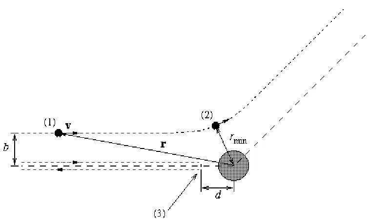
Figure 2.1 The trajectory of a particle undergoing Rutherford scattering, showing the impact parameter b, the minimum separation distance rmin, and the distance of closest approach d.

The geometry for Rutherford scattering can be seen in Figure (2.1). A charged

particle approaches the target nucleus along a trajectory that would pass a distance b from

the nucleus in the absence of the Coulomb force; this distance is known as the impact

parameter. Far from the nucleus at point (1), the incident particle has negligible Coulomb

potential energy, so all of its energy is accounted for in its kinetic energy

2 0 0

2 1

mv

E = , (2.6)

where m and v0 are the mass and initial velocity of the particle, respectively. At this point

the particle’s angular momentum relative to the nucleus is given by

b mv

m = ₀

´ = r v

l , (2.7)

(19)

point (2). For a positively charged particle, the absolute minimum value for rmin occurs in

a head-on collision course (corresponding to b=0) at the point (3), when the particle

comes to rest and then changes direction. At this point, all of the initial kinetic energy of

the particle has been converted into Coulomb potential energy, so

d zZe mv 2 2 0 4 1 2 1 0 =

pe , (2.8)

where ze is the charge of the particle, Ze is the charge of the nucleus, and d is the distance

of closest approach as shown in Figure (2.1). This distance of closest approach

corresponds to the absolute minimum value for rmin.

Since the electron is interacting with a nucleus much more massive than itself,

and since this is an elastic scattering event, the magnitude of the electron’s momentum

before and after the event can be taken to be the same. Thus, if pI and pf are the initial

and final momentum of the electron, respectively, we have that p_f = p_i =mv₀. The

change in momentum vector shown in Figure (2.2) then has magnitude

2 sin 2mv₀ f p=

D , (2.9)

where f is the scattering angle for the incident particle. Using Newton’s second law,

dt dp

F = , we can now write the net impulse of the Coulomb force in the direction of Dp

as dt r zZe dt F dp

p=

ò

=

ò

=

ò

D ₂

0 2

4pe , (2.10)

(20)

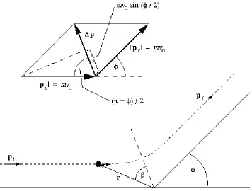
Figure 2.2 The hyperbolic path of a particle undergoing Rutherford scattering. The coordinates of the particle at any given instant are r, b. The vector representing the change in momentum, Dp, bisects the angle in the upper figure with magnitude (p - f).

2 0

2

4 r

zZe F

pe

= (2.11)

is the Coulomb force between the nucleus and the incident particle. If we sum the

infinitesimal momentum vectors indicated in the first integral of Equation (2.10), only the

components of these vectors oriented along the direction of the angle bisector (dashed

line) in Figure (2.2) will contribute to Dp. Thus, we can write

dt r zZe

p=

ò

D ₂

0 2 _cos

4

b

(21)

where b is the angle between the bisector and the particle’s position vector r (see Figure

2.2). The integral in this expression should be evaluated over the temporal limits t =-¥

to t=¥, which correspond to the angular limits b =-(p -f) 2 to b =+(p -f) 2.

The instantaneous velocity vector v for the particle can be written in terms of

radial and tangential components as

β r

v ˆ ˆ

dt d r dt

dr ₊ b

= , (2.13)

where rˆ and βˆ are the radial and tangential unit vectors, respectively. The instantaneous

angular momentum of the particle relative to the nucleus is therefore given by

dt d mr

m ₌ 2 b

´ = r v

l . (2.14)

Since the initial angular momentum is just mv0b, conservation of angular momentum

gives

dt d mr b

mv 2 b

0 = , (2.15)

so that db b v r dt 0 2 1

= . (2.16)

Substituting this result into Equation (2.12) gives

( )

b b pe f p f p

ò

-+ - -=

D ₍( ₎)_//₂2 0

0 2

cos 1

4 v b d

zZe

p , (2.17)

which simplifies to

÷ ø ö ç è æ = D 2 cos

2 ₀ ₀

2 _f

pe v b zZe

(22)

Now, combining this last result with Equations (2.8) and (2.9), we obtain the Rutherford

scattering formula:

d b 2 2 cot ÷=

ø ö ç è

æf _. _(2.19)

This formula relates the scattering angle, f, to the impact parameter, b, and the distance

of closest approach, d. Although this derivation assumes a positively charged particle in

defining the distance of closest approach, the general form of the Rutherford scattering

(23)

3 Modeling Electron Interactions With Solids

3.1 Assumptions of the Model

In modeling the interaction of an electron with a solid, the basic idea is to trace

the incident electron from one distinct scattering event to the next until it either leaves the

solid or loses all of its energy. The model must determine how the trajectory and energy

of the electron are affected at each event, and how far the electron will travel between

successive scattering events. In reality, each scattering event could be either elastic or

inelastic, so changes in the energy and trajectory of the electron should be computed

based on the specific sequence of scattering events experienced by the particular electron.

In practice, however, all scattering events are not equally important in terms of their

effect on the trajectory or energy of the electron. Therefore, we make two important

assumptions suggested by Joy (1995) in developing our model.

First, we assume that only elastic scattering events are important in determining

the path of an electron. Elastic scattering, which is described by the Rutherford scattering

formula, typically results in angular deflections in the range 5 to 10 degrees. Inelastic

scattering, on the other hand, causes the incident electron to lose energy to the solid, but

causes relatively little angular deflection. In fact, the angular deflection in an inelastic

scattering event is of the order DE E (that is, the ratio of energy loss, DE, to the energy

of the electron, E). An inelastic scattering event that results in a larger energy loss will

(24)

about 1/DE (Egerton, 1986). Since only a very small fraction of inelastic events produce

significant angular deflections, elastic scattering events dominate in determining the

spatial distribution of the interaction. Therefore, ignoring the trajectory-changing effects

of inelastic scattering produces little error.

We also assume that the electron loses energy continuously along its trajectory

rather than losing energy in discrete amounts through inelastic scattering events. While

this assumption is consistent with some energy-loss mechanisms, such as the production

of Bremsstrahlung by the slowing down of the incident electron through its interactions

with other electrons in the solid, most energy losses are associated with a specific event,

such as the production of an inner shell ionization. However, considering all energy

losses along the path of an incident electron collectively leads to a convenient and simple

expression that accounts for all energy-loss phenomena. This simplification is based on a

continuous slowing-down approximation and is attributed to Bethe (1930). Bethe showed

that the rate at which an electron loses energy to a solid could be expressed as

÷ ø ö ç è æ × -= J E AE ZN e ds

dE ₂_p 4 _Ar_ln g _, _(3.1)

where E is energy of the electron, s is the distance the electron has traveled, e is the

electron charge, and NA is Avogadro’s number. The quantities Z, A, and r are the atomic

number, atomic weight, and density of the solid, respectively, and J is the mean

ionization potential of the solid. The constant g in the logarithmic term has the value

(25)

A

ZN_Ar , which gives the number of electrons per unit volume in the solid. It makes

sense that the total number of inelastic collisions suffered by an incident electron, and

thus the stopping power of the target, should be proportional to this term. Most current

electron scattering models implement Bethe’s model of continuous energy loss in one

form or another.

At this point we can develop a “single scattering” model, in which we account for

all elastic scattering events experienced by an electron along its trajectory. Following this

approach, we would use a screened Rutherford elastic cross section to determine the

“mean free path” for the electron, which represents the average distance the electron will

travel between successive elastic scattering events. From the mean free path we would

calculate the distance traveled between one particular scattering event and the next using

Monte Carlo techniques. Such a model gives excellent results, but we can greatly reduce

the amount of computation required with insignificant loss of accuracy by using a “plural

scattering” model instead (Joy, 1995). A plural scattering model attempts to compute the

net effect produced by a number of successive scattering events at each step of the

simulation, and is best suited to problems that involve incident electrons traveling into a

bulk specimens (as opposed to thin film specimens).

3.2 Basic Plural Scattering Model

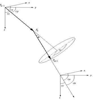
Figure (3.1) illustrates the geometry for an electron scattering simulation. Here,

(26)

traveled to Pn from a previous scattering event at Pn-1. The primary task of the model,

then, is to calculate the coordinates of the point Pn+1 to which the electron travels as a

result of the scattering event at Pn. When the electron arrives at Pn, we know its energy E,

and its trajectory as given by the direction cosines cx, cy, and cz. These direction cosines

are defined as the cosines of the angles between the velocity (trajectory) vector and the x,

y, and z axes. The x, y, and z axes are defined with the convention that the xy-plane

corresponds to the solid’s surface and the z-axis is directed into the solid.

(27)

In order to calculate the position of the new scattering point Pn+1, we first need to

determine the distance between Pn and Pn+1. Using Bethe’s continuous energy-loss

approximation we can determine the total distance (in cm) the electron will travel through

the material as

dE R E ds dE B

ò

ú ú û ù ê ê ë é-= 0 0 1 (3.2)

where E0 is the initial energy of the incident electron, and (dE/ds) is the Bethe stopping

power given in Equation (3.1). Note, however, that substitution of the original Bethe

equation (3.1) into the integral in Equation (3.2) will result in a division by zero when the

argument of the logarithm term is identical to one. To remedy this we instead use a

modified version of the Bethe stopping power proposed by Joy and Luo (1989):

÷ ø ö ç è æ + × × -= J J E AE Z ds

dE 1.166( 0.85 )

ln 500

,

78 r (keV/cm). (3.3)

Also, rather than maintaining a table of values for the mean ionization potential, we can

approximate this quantity with good accuracy using a convenient relationship proposed

by Berger and Seltzer (1964):

3 19 . 0 10 5 . 58 76 .

9 _÷_´

-ø ö ç è æ ₊ = Z Z

J (keV). (3.4)

The Bethe range RB can now be divided into an arbitrary but sufficiently large number of

steps of equal length (Joy, 1995) to give the distance between one scattering event and

the next.

The stopping power can also be used to determine the energy of the electron at

(28)

ò

D - ÷ ø ö ç è æ -= n s n n ds ds dE E

E ₁ , (3.5)

where En-1 is the energy at Pn-1, Dsn is the path traveled between Pn-1 and Pn, and (dE/ds)

is the modified Bethe stopping power from Equation (3.3).

To determine the scattering angle, a randomized Rutherford-type scattering

formula can be applied to calculate a scattering angle for each event. One such scattering

formula suggested by Mykelbust et al. (1976) is given by

÷ ø ö ç è æ -= ÷ ø ö ç è

æ 1 ₁

2 tan L R E F

f _, _(3.6)

where f represents the scattering angle, E is the instantaneous energy of the electron (in

keV), and RL is a random number in the interval [0, 1]. The quantity F embodies the

parameters p and b in Equation (2.19), and is given by

0 0 0072 . 0 P ZE

F = , (3.7)

where

4 . 0 0 0.394 Z

P = × (3.8)

is a parameter that has been fitted to give the correct backscatter coefficient for a flat

specimen. Now, if we consider our random variable to be h =tan(f 2), then Equation

(3.6) corresponds to Equation (2.4) after it has been solved for h.

Since the electron can scatter (with equal probability) to any point on the base of

(29)

where RL is a new and independent random number in the interval [0, 1]. We now have

all the information (step length, scattering angle f, and azimuthal angle y) that we need

to relate Pn+1 to Pn.

3.3 Implementation Details

Before we summarize the complete plural scattering algorithm, we need to

provide some essential details required for the implementation. For instance, in order to

evaluate the integral expressions required by our plural scattering model, we will need to

incorporate some numerical integration techniques into our simulation package.

To evaluate the integral in Equation (3.2), for instance, we use a composite

Simpson’s rule numerical integration (Burden and Faires, 1993) as follows:

§ Define a function stop_pwr() based on Equation (3.3):

÷ ø ö ç è æ + × × = -= J J E AE Z ds dE E pwr

stop_ ( ) 78,500 r ln 1.166( 0.85 ) (3.10)

§ Define the integrand as

) ( _ 1 ) ( E pwr stop E

f = (3.11)

§ Choose an even number of subintervals, n, for the quadrature.

§ Define the width of each subinterval as

n E n E

h=( ₀ -0) = ₀ , (3.12)

where E0 and 0 are the two endpoints for the integral.

§ Set x_j = jh for j =0,1,...,N (3.13)

§ Now the value of the Bethe range can be approximated as

ú ù ê é + + +

@ (0) 2(

å

2)-1 ( 2 ) 4

å

2 ( 2 _-1) ( 0)

n n

j j

B f f x f x f E

h

(30)

The error for this approximation can be written as ) ( 180 ) 4 ( 4 0 _h _f _m

E

Err= , (3.15)

where m is some particular value on the interval [0, E0].

For Equation (3.5), which is actually an initial value problem, we apply a fourth

order Runge-Kutta method (Burden and Faires, 1993). We want to approximate the

solution to

) ( _ )

(s stop pwr E

E¢ =- , 0£s£R_B, E(0)=E₀, (3.16)

at (N + 1) equally spaced numbers (s[i] for i = 0,1, …, N) in the interval [0, RB]. (Note

that s represents the distance the electron has traveled through the solid, RB represents the

Bethe range, and E0 is the initial energy of the electron.) The approximation to E(s) at

each s[i] will be assigned to E[i]. The Runge-Kutta method of order four can be

summarized as follows:

§ Set the step length to

N R

h= _B (3.17)

§ The initial conditions are

0 ] 0

[ =

s , E[0]=E₀ (3.18)

§ Fori = 1, 2, …, N do

§ Set ]) 1 [ ( _

1 =h×stop pwr E i

-V (3.19) ) 2 ] 1 [ ( _ ₁

2 h stop pwr E i V

V = × - - (3.20)

) 2 ] 1 [ ( _ ₂

V = × - - (3.21)

) ] 1 [ ( _ ₃

(31)

(

1 2 2 2 3 4

)

6 1 ] 1 [ ]

[i E i V V V V

E = - - + + + (3.23)

ih i

s[]= (3.24)

§ Endfor loop

Note that the local truncation error for a Runge-Kutta method of order four is O(h4).

Using this method, we can obtain an approximate value for the energy at each step of our

simulation. These energy values can, in turn, be used to calculate the scattering angle at

each step using Equation (3.7).

Now we are ready to summarize the steps involved in our basic plural scattering

simulation. The following pseudo code best describes the algorithm:

§ Initialize variables representing the properties of the solid: the atomic number Z, the atomic weight A, and the density r.

§ Initialize variables representing the properties of the electron: the initial

energy E0 and the initial trajectory c. The initial position can be set to

(

0,0,0

)

=

x .

§ Set the number of steps for the electron trajectory simulation to N.

§ Calculate J according to Equation (3.4).

§ Calculate the Bethe range RB using Equations (3.10) – (3.14). § Set the step size for the simulation at step=R_B N.

§ Calculate the scattering parameters P0 and F using Equations (3.7) and (3.8).

§ Fori = 1, 2, … Ndo

§ Generate a random number RL, then calculate f using Equation (3.6) with

E = E[i].

§ Generate another random number RL, then calculate y using Equation

(32)

§ Find a vector v that is orthogonal to c. We can easily accomplish this by letting v₌c_´xˆ. (On the rare occasion that c and x are perfectly parallel, we can let v=c´yˆ.)

§ Let cnew =c, then rotate cnew about v by f radians.

§ Rotate this cnew about c by y radians. This is the new trajectory vector. § Let x_new =x+step×c_new.

§ If i<N(if this was not the last step)

§ Reassign position and trajectory vectors: x¬x_new and c¬c_new.

§ Compute the energy for the next step, E[i], using E[i-1] and Equations (3.19) through (3.23).

§ Else (iºN)

§ Set E[N] = 0.

§ Go to end of for loop

§ End if-else statement

§ If xz <0 (if the electron has left the solid; i.e., if it has “backscattered”)

§ Go to end of for loop

§ End if statement

§ End for loop

§ Output exit trajectory cnew and exit energy E[i].

This plural scattering algorithm, which will henceforth be referred to as Scatter1,

is the basis for all of the electron trajectory simulation programs that we implemented. In

the next chapter, we describe the experiments we conducted using this code, and the

subsequent modifications that we made in order to improve the correlation between the

(33)

4 Comparisons With Experimental Data

4.1 Scatter1

Output vs. Experimental Data

As discussed previously, an incident electron will continue to propagate through a

solid, potentially undergoing thousands of scattering events, until it has either lost all of

its energy or it has left the target material as a backscattered electron. As the name

implies, backscattered electrons are those incident electrons that are scattered in the target

in such a way as to be collectible by some detector placed on the incident beam side of

the targeted material. The important values considered in this research are the backscatter

coefficient, which is the ratio of backscattered electrons to incident electrons, and the

energy and exit angle of the backscattered electrons.

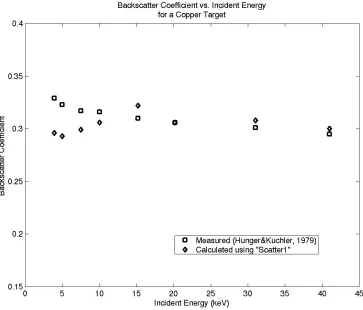
Now that we have a working model, we can use it as discussed in Section 2.1 to

estimate probabilities related to our problem. In particular, we can use our plural

scattering algorithm Scatter1 to make an estimate of the backscatter coefficient h by

simulating a large number of electrons that enter a copper slab with normal incidence and

counting the number of electrons that are ejected. Since we have experimentally

measured values for h for several different values of incident energy (E0) in the range

3.93 to 41.0 keV (Hunger and Kuchler, 1979), we can run our simulations using these

same energy values and compare the resulting estimates of h with the experimental

values. We performed this experiment for a copper target, using 1000 trajectory

(34)

between the measured values and the simulation values to be 4.6%. The results of this

experiment are displayed graphically in Figure (4.1).

Figure 4.1 A plot illustrating the variation of the backscatter coefficient, h, with the incident energy of the electron. Each “calculated” data point is based on 1000 simulations.

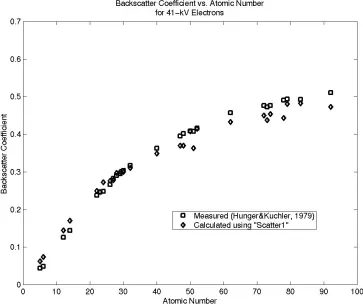
In a second experiment we used Scatter1 to predict the backscatter coefficient for

various different elements. For each data point in this experiment, we used 1000 41-keV

electrons and counted the number of electrons that were ejected. Again the results were

compared to the values measured by Hunger and Kuchler, but this time we found the

(35)

Figure 4.2 A plot illustrating the variation of the backscatter coefficient, h, with the atomic number of the target solid. Each “calculated” data point is based on 1000 simulations.

4.2 Development and Testing of

Scatter2

Seeking to improve upon the backscatter coefficient predictions generated with

Scatter1, we implemented a second scattering algorithm based on a slightly different

scattering formula. This scattering formula is an alternate version of the Rutherford

formula given in Equation (3.7) in which the scattering factor F is related to the

“minimum scattering angle” f0 by

0 0

2

tan E

F ÷×

ø ö ç è æ

(36)

÷ ø ö ç è æ -÷ ø ö ç è æ = ÷ ø ö ç è

æ 1 ₁

2 tan 2

tan 0 0

L

R E E

f

f _. _(4.2)

We can relate the minimum scattering angle to the backscatter coefficient, itself, as

suggested by Love et al. (1977) using a relation proposed by Joy (1996):

3 2

0 ₀_.₀₁₆₆₉₇ ₀_.₅₅₁₀₈ ₀_.₉₆₇₇₇ ₁_.₈₈₄₆

2

tan f ÷= + h- h + h

ø ö ç è

æ _. _(4.3)

Now, we just need an easy way to estimate what the backscatter coefficient should be so

we can use that value in evaluating our new scattering formula. In the same paper in

which Hunger and Kuchler present their experimental data on backscatter coefficients,

they propose an analytical expression that accomplishes just this. The formula predicts

the backscatter coefficient h (at normal beam incidence) using both the atomic number Z

and the incident energy E0:

), ( )

,

(Z E₀ =E₀m(Z)×C Z

h (4.4)

where

Z Z

m( )=0.1382-0.9211 (4.5)

and

3 2 ₀_.₀₁₄₉₁_(ln ₎

) (ln 1292 . 0 ln 2236 . 0 1904 . 0 )

(Z Z Z Z

C = - + - . (4.6)

Our second algorithm, which we call Scatter2, is essentially identical to Scatter1,

except that the quantity F is calculated using Equation (4.1) in conjunction with

Equations (4.3) through (4.6). Note that, as before, the quantity F only needs to be

(37)

Figure 4.3 Another plot illustrating the variation of the backscatter coefficient, h, with the incident energy of the electron. This time, the data generated by both Scatter1 and Scatter2 are displayed.

We performed the first experiment described in Section 4.1 using Scatter2, and

again using 1000 trajectory simulations for each value of incident energy. This time we

found the average percent difference between the measured values and the simulation

values to be 2.48%, which represents a significant improvement over the results of

Scatter1. Figure (4.3) illustrates the results obtained for the backscatter coefficient vs.

incident energy experiments for both Scatter1 and Scatter2.

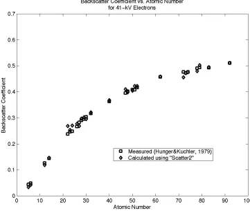
Scatter2 also outperforms Scatter1 for the backscatter coefficient vs. atomic

number experiment. In this case, the average percent difference between the simulation

(38)

comes from the first few data points, where the value of h is relatively small and the

value for percent difference can therefore become quite large. If we omit the first two

data points, which correspond to solids with atomic numbers less than 10, the average

percent difference becomes 3.34%. The results of this experiment are shown in Figure

(4.4).

(39)

predict other interesting quantities, however. For instance, while the Hunger-Kuchler

formula can only predict the backscatter coefficient for electrons entering a solid with

normal incidence, Scatter2 can predict the situtation for electrons entering the solid at any

angle.

Myklebust et al. (1976) measured the backscatter coefficient as it varied with

specimen tilt for 30-keV electrons incident on an iron alloy containing 3.22% silicon.

Here, “tilt” refers to the angle through which the specimen surface is rotated relative to

the incident electron beam. A tilt of 0 degrees would correspond to normal incidence,

whereas a tilt of 90 degrees would correspond to grazing incidence.

(40)

So, we once again used Scatter2 to calculate backscatter coefficients, but this time

we simulated trajectories for 30-keV electrons using entry angles ranging from 0 to 80

degrees in 10-degree increments. As shown in Figure (4.5), the calculated backscatter

coefficients predict the experimentally measured values very well. In fact the percent

difference between the calculated values and the measured values is about 3.83%.

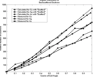
The Scatter2 program can also be used to predict exit angles for backscattered

electrons. Since we have some experimentally determined angular distributions for

electrons backscattered from copper, silver, and gold (Bishop, 1966), we calculated

angular distributions for these materials using Scatter2. Essentially, the procedure we

followed was to model 10,000 30-keV electrons for each type of target. We then

examined the trajectory of each backscattered electron, and calculated the cosine of the

angle q between this trajectory and the surface normal. Next, we set up 10 counting bins

corresponding to 10 equal divisions of the interval 0 to 1 (where 0 to 1 is the range of

possible cosine values). Finally, for each backscattered electron, we just incremented the

count in the bin corresponding to the value of cos(q). In order to compare this calculated

data with the measured data, we plotted the number of electrons in the bin corresponding

to 0.0£cos(q)£0.1 at the x-coordinate 0.1, and so on. Since the measured data provided

by Bishop only shows the relative electron counts (i.e., no scale is provided for the

electron count data), it was necessary to match the predicted curves to the measured

curves in a qualitative way. Figure (4.6) shows that the relative spacing and shapes of the

(41)

Figure 4.6 A plot illustrating the angular distribution of backscattered electrons. The data was measured by Bishop (1966) using 30-keV incident electrons.

Thus, Scatter2 does a reasonably good job of predicting backscatter coefficients

and angular distributions of backscattered electrons, but we also need to predict with

reasonable accuracy the energy distributions of backscattered electrons. Bishop made

some measurements of the “energy spectrum” dh

( )

q dW vs. W, where h

( )

q is the

relative number of backscattered electrons with exit angle q, and W is the ratio of the exit

energy to the incident energy of the electron; therefore, we constructed a simulation

experiment to derive an energy spectrum using Scatter2.

(42)

electron, and calculated the angle q between this trajectory and the surface normal.

Bishop examined backscattered electrons for which q = 45 degrees, so we considered

electrons for which 40£q £50. Next, we set up 10 counting bins corresponding to 10

equal divisions of the interval 0 to 1 (where 0 to 1 is the range of possible values for W).

For each backscattered electron, we just incremented the count in the bin corresponding

to the value of W. At this point, plotting the number of electrons in the bin corresponding

to 0.0£W £0.1 at the x-coordinate 0.1, and so on, would give a curve representing h vs.

W. However, we need a plot of dh/dW vs. W to compare with the measured data of

Bishop. To get such a curve, we used a three-point numerical differentiation rule (Burden

and Faires, 1993). Figure (4.7) shows the results of this experiment, and unfortunately it

(43)

Figure 4.7 A plot illustrating the energy spectrum of backscattered electrons. The values actually plotted are values of dh/dW vs. W, where h is the ratio of electrons ejected at 45 degrees (from the surface normal) to incident electrons, and W = E/E0. The data was measured by Bishop (1966) using 30-keV electrons.

4.3 Development and Testing of

Scatter3

,

Scatter4

, and

Scatter6

Since Myklebust et al. were able to improve their predictions of backscattered

electron energy distributions by using an energy-dependent variable step length in their

simulation algorithm, we attempted to incorporate this technique into our own algorithm.

The basic idea can be summarized as follows. Assuming a trajectory comprised of 60

steps of equal length, use a Runge-Kutta method as before to calculate the energy at each

(44)

corresponding to that step. This fraction was chosen because with it, the sum of 60

variable-length steps gives a total trajectory length that is approximately equal to the

original Bethe range (Myklebust et al., 1976).

By incorporating this variable step length technique into Scatter2, we created a

new algorithm, which we called Scatter3. Unfortunately, Scatter3 performed terribly

when used to predict backscatter coefficients (see Figure 4.8). Upon closer examination

of the algorithm described by Myklebust et al. (the NBS code), we discovered that this

(45)

Equation 3.7), except that the scattering parameter P0 (compare with Equation 3.9) is

given by

4 . 0 0 0.263 Z

P = × . (4.7)

Apparently the enhancements featured in Scatter2 are not readily applicable to the NBS

code because of subtle differences such as this in corresponding parts of the two

algorithms.

Still hoping to improve our predictions for backscattered electron energy

distributions, we made the variable step length modifications to Scatter1. Then, after

making the appropriate change to the scattering parameter P0 by replacing Equation (3.9)

with Equation (4.7), we named this new algorithm Scatter4.

We also created an algorithm that uses the average energy between steps for the

scattering formula calculation. That is, at step i, this algorithm uses the value

2 ] 1 [ ]

[ + +

= E i E i

E (4.8)

in evaluating the scattering formula (Equation 3.7). This modification was made based on

the suggestion of Myklebust et al. (1976) to use the midpoint energy at each step. Finding

the midpoint energy would require doubling the number of steps in the Runge-Kutta

subroutine. Finding the mean energy, it was decided, would give a comparable value but

would require significantly less computation. This algorithm, which is otherwise identical

to Scatter4, we called Scatter6.

Scatter4 and Scatter6 both outperform the previous algorithms in predicting the

(46)

closely match those of the experimentally measured energy spectrums. The magnitudes

of the calculated curves (for Scatter4 and Scatter6) show significant (but approximately

equal) deviation from the measured curves, but the estimated errors for the experimental

values themselves are of the order of 10% (Bishop, 1966).

Figure 4.9 A plot illustrating the energy spectrum of electrons backscattered from copper. The values actually plotted are values of dh/dW vs. W, where h is the ratio of electrons ejected at 45 degrees (from the surface normal) to incident electrons, and W = E/E0. The data was measured by Bishop (1966) using

(47)

Figure 4.10 A plot illustrating the energy spectrum of electrons backscattered from silver. The values actually plotted are values of dh/dW vs. W, where h is the ratio of electrons ejected at 45 degrees (from the surface normal) to incident electrons, and W = E/E0. The data was measured by Bishop (1966) using

(48)

Figure 4.11 A plot illustrating the energy spectrum of electrons backscattered from gold. The values actually plotted are values of dh/dW vs. W, where h is the ratio of electrons ejected at 45 degrees (from the surface normal) to incident electrons, and W = E/E0. The data was measured by Bishop (1966) using

30-keV electrons.

As for predictions of the backscatter coefficient, Scatter4 and Scatter6 both fall

somewhat behind the capabilities of Scatter2. When applied to the problem of predicting

the backscatter coefficient from copper at various incident energies, the average percent

difference between Scatter4 data and measured data is 5.72% (see Figure 4.12).

However, the average percent difference between Scatter6 data and measured data for

this experiment is 2.92% (see Figure 4.13). Thus, Scatter6 nearly matches the accuracy of

(49)

(50)

When applied to the problem of predicting the backscatter coefficient for 41-keV

electrons incident on various elements, Scatter6 again performs better than Scatter4, but

both of these new algorithm again fall behind Scatter2. The average percent difference

between Scatter4 and the measured data is 10.97% (see Figure 4.14), while the average

percent difference between Scatter6 and the measured data is 9.02% (Figure 4.15).

Again, much of this error is attributed to the first two data points, which have small

magnitude. If we eliminate these two data points from our percent difference calculation,

(51)

(52)

Next, we used Scatter4 and Scatter6 to predict the backscatter coefficient of

30-keV electrons incident on copper at various angles. As seen in Figure (4.16), both of the

curves constructed from the predicted data have the correct shape, but both have slightly

less accurate values for the magnitudes of the backscatter coefficients compared to

Scatter2. In fact the average percent difference between the calculated and measured

backscatter coefficients in this case is about 8.83% for Scatter4 and about 7.92% for

(53)

Figure 4.16 A plot illustrating the variation of the backscatter coefficient, h, with the incident angle of the electron. Each “calculated” data point is based on 1000 simulations of 30-keV electrons. The measured data comes from Myklebust et al. (1976).

Finally, we used Scatter4 and Scatter6 to predict the exit angles of electrons

backscattered from copper, silver, and gold. Both do a reasonable job of predicting the

angular distributions, but as is the case with Scatter2, it is difficult to compare the data

from the predictions with the measured data because explicit information about the

scaling of the data is not available in the reference. However, it is clear from Figures

(4.17) and (4.18) that the relative magnitudes and shapes of the calculated distribution

(54)

(55)

Figure 4.18 A plot illustrating the angular distribution of backscattered electrons. The data was measured by Bishop (1966) using 30-keV incident electrons.

4.4 Concluding Remarks

In an attempt to produce a single algorithm capable of predicting all of the desired

qualities of backscattered electrons, several other algorithms were developed and tested.

Some of these (Scatter7 and Scatter8) were based on the NBS strategy of using the

mid-point energy along each step for the scattering formula calculations (Myklebust et al.,

1976). Others (Scatter5) attempted to reconcile the discrepancies seen in the data

generated by Scatter3 by adjusting coefficients in the scattering formula. Unfortunately,

(56)

Scatter2 and Scatter4. Out of all the algorithms we implemented Scatter6 comes closest

to being an all-purpose algorithm, as it predicts values within about 8% of most of the

(57)

5 Conclusions and Future Plans

As pointed out by Joy (1996), it is “an apparently irresistible temptation in Monte

Carlo modeling” to implement an all-purpose computer program that can answer any

question about any effect related to a given phenomenon. Unfortunately, in the case of

the electron backscattering problem, this proves to be all but impossible. With the

Scatter2 algorithm, we can calculate with excellent accuracy backscatter coefficients and

angular distributions, but we fail completely to predict the energy spectra seen in

experiments. With the Scatter4 algorithm, we can get much better predictions of energy

spectra, but the accuracy of our backscatter coefficient estimates declines. Scatter6 does

not predict the shapes of the energy spectra as well as Scatter4, and does not predict

backscatter coefficient data as well as Scatter2, but it seems to be the best “all-around”

algorithm in the sense that it minimizes the total error if we consider all the experiments

together. Thus, it would seem that Joy’s synopsis is correct: “A Monte Carlo model is

most efficient and effective when it is constructed as a special tool to solve a particular

[specific] problem.”

Concurrent with the research presented in this thesis, a California-based company

called Calabazas Creek Research (CCR) has been working on a general-purpose charged

particle modeling code that is based on adaptive meshing and a finite element approach to

solving the Maxwell equations. This code models the movement of charged particles

(typically electrons) through user-specified fields and physical geometries, and calculates

(58)

collisions with surfaces contained in the model. In particular, the model needs to account

for the so-called “secondary emission” that results from the interaction of electrons with

surfaces. The research presented in this thesis was actually conducted with this particular

application in mind.

Since most energetic secondary electrons are actually backscattered primary

electrons (rather than “true” secondary electrons), we focused our efforts on predicting

the behavior of backscattered electrons. As discussed in the preceeding chapters of this

thesis, such predictions can be accomplished by simulating the trajectories of electrons as

they enter and move through a solid, and examining those electrons that happen to exit,

or backscatter, from the solid. The next logical step for this research process is to develop

and implement a subroutine for the CCR code that is based on the algorithms discussed in

this thesis. This subroutine should take as input all the electron data structures that are

incident upon surfaces within the model at a given instant, and return as output a new set

(59)

Bibliography

Berger, M.J., and Seltzer, S.M. Studies in Penetration of Charged Particles in Matter. Nuclear Science Series Report #39, NAS-NRC Publication 1133 (Natl. Acad. Sci.: Washington, D.C.), p. 205, 1964.

Bethe, H.A. “Zur Theorie des Durchgangs Schneller Korpuskularstrahlen durch Materie.” Annalen der Physik 5:5, pp. 325-400, 1930.

Bishop, H.E. “Some Electron Backscattering Measurements for Solid Targets.” International Symposium on X-ray Optics and X-ray Microanalysis (4th: 1965: Orsay, France), 153-8, 1966.

Burden, Richard L., and Faires, J.Douglas. Numerical Analysis. 5th Ed. PWS Publishing Co., Boston, 1993.

Egerton, R.F. Electron Energy –Loss Spectroscopy in the Electron Microscope. New

York: Plenum Press, 1986.

Hammersley, J.M., and Handscomb, D.C. Monte Carlo Methods. New York: Wiley,

1964.

Hunger, H.-J., and Kuchler, L. “Measurements of the Electron Backscattering Coefficient

for Quantitative EPMA in the Energy Range of 4 to 40 keV.” Physica Status

Solidi (a) 56, K45-48, 1979.

Joy, David C. Monte Carlo Methods for Electron Microscopy and Microanalysis. New

York: Oxford UP, 1995.

Joy, D.C., and Luo, S. “An Empirical Stopping Power Relationship for Low-Energy Electrons.” Scanning, Vol. 11, 176-180, 1989.

Krane, Kenneth S. Introductory Nuclear Physics. New York: Wiley, 1988.

Larson, Harold J. Introduction to Probability Theory and Statistical Inference. New York: Wiley, 1982.

Love, G., Cox, M.G.C., and Scott, V.D. “A Simple Monte Carlo Method for Simulating Electron-Solid Interactions and its Application to Electron Probe Microanalysis.” Journal of Physics D: Applied Physics 10:1, pp. 7-23, 1977.

Myklebust, Robert L., Newbury, Dale E., and Yakowitz, Harvey. “NBS Monte Carlo

Electron Trajectory Calculation Program” (1976) in Use of Monte Carlo

Calculations in Electron Probe Microanalysis and Scanning Electron

Monte Carlo Techniques for Predicting Electron Backscattering

Abstract

Monte Carlo Techniques for Predicting Electron

Backscattering

Dustin F. Kapraun

Department of Physics

Approved By:

Dedication

Biography

Acknowledgments

Table of Contents

List of Figures

1

Introduction

2

Theoretical Background

2.1

Monte Carlo Methods

ò

ò

ò

2.2

Random Numbers and Pseudorandom Numbers

2.3

Rutherford Scattering

ò

ò

ò

ò

( )

ò

3

Modeling Electron Interactions With Solids

3.1

Assumptions of the Model

3.2

Basic Plural Scattering Model

ò

ò

3.3

Implementation Details

å

å

(

)

(

)

4

Comparisons With Experimental Data

4.1

Scatter1