ABSTRACT
HAMILTON, TIMOTHY LAURENCE. A Multi-Level Residential Sorting Model with an Application to Cost of Living Indices. (Under the direction of Daniel Phaneuf.)
Sorting models to date have operated at the macro level or micro level. Regardless of the
scale, all existing sorting models analyze a single choice from a single set of alternatives.
Intu-ition suggests, however, that households choose a city and subsequently select a neighborhood
within that city. This stylized reality is absent from conventional sorting models, which ignore
information at one of these stages. In addition, due to the size of the full choice set, capturing
this entire sorting process in a single model can be prohibitive in terms of computation and data
collection. I use the theory of two-stage budgeting to develop an empirically feasible sorting
model that more accurately replicates household behavior. Empirically, I focus on the cost of
air pollution. Results point to an additional tradeoff between air pollution and
neighborhood-level amenities that increases the marginal willingness to pay for clean air by a considerable
amount. I also show that allowing for heterogeneity in preferences for local public goods has a
considerable impact on the estimated value of clean air.
This dissertation also explores an application of the model in which I construct spatially
explicit measures of the cost of living that can be used to adjust income and calculate a broad
measure of welfare. The analysis focuses on the distribution of such welfare across the
popu-lation, as well the change in this distribution followings simulated reductions pollution
concen-trations. Empirical results suggest that accounting for public goods leads to a distribution of
adjusted income that has a wider spread than that of pure monetary income. This implies that
households with less income tend to face higher costs of living, determined by an inferior set of
A Multi-Level Residential Sorting Model with an Application to Cost of Living Indices
by
Timothy Laurence Hamilton
A dissertation submitted to the Graduate Faculty of North Carolina State University
in partial fulfillment of the requirements for the Degree of
Doctor of Philosophy
Economics
Raleigh, North Carolina
2012
APPROVED BY:
Laura Taylor Walter Thurman
Christopher Timmins Daniel Phaneuf
DEDICATION
To my parents, who even through times of oblivion offered nothing short of unconditional love
BIOGRAPHY
The author was born the second of three children to a modest family in the bucolic town of
Hudson, MA. He was afforded the opportunity of a strong public education and eventually took
his Bachelor’s degree from Bentley College. Following graduation, he immediately enrolled as
a doctoral student at North Carolina State University to pursue a degree in economics. A
rigorous approach to economic theory, modeling and econometric methods served him well,
as he focused his attention on environmental economics, exploring technical approaches and
ACKNOWLEDGEMENTS
I extend my deepest gratitude to my parents, to whom this dissertation is dedicated, my
brothers, my family, and my friends who have been there throughout and have contributed so
heavily to preserving my sanity and motivation. I thank the faculty of North Carolina State
University who have supplied me with the skills and techniques to finish this document. I thank
my fellow graduate students who struggled alongside me, and those that continue to do so. I
thank Chris Timmins and Wally Thurman, who have offered endless knowledge and expertise
to get me to this point. I thank Laura Taylor, who has provided immeasurable support for
this document and beyond. Finally, I thank my advisor, Dan Phaneuf, without whom this
dissertation would not have been possible. His dedication, ingenuity, and perpetual guidance
TABLE OF CONTENTS
List of Tables . . . vii
List of Figures . . . ix
Chapter 1 Introduction . . . 1
Chapter 2 Literature Review . . . 6
2.1 Residential Sorting Models . . . 6
2.1.1 Development of Literature . . . 7
2.1.2 Issues in Applications . . . 14
Chapter 3 Theoretical Model . . . 19
3.1 Generalized Horizontal Sorting Model . . . 19
3.2 Two-Stage Budgeting . . . 22
3.2.1 Price Aggregation . . . 23
3.2.2 Decentralisability . . . 24
3.3 Two-Stage Residential Sorting Model . . . 25
3.4 Empirical Basis . . . 28
3.4.1 Conditions for Two-Stage Budgeting . . . 29
3.4.2 A Two-Stage Model . . . 33
3.4.3 Construction of Index . . . 34
3.4.4 Normalization of Tract-Level Fixed Effects . . . 38
3.4.5 Macro Stage Sorting . . . 40
Chapter 4 Data and Preliminary Estimation. . . 43
4.1 Data . . . 43
4.2 Estimation Approach . . . 46
4.2.1 Housing Prices . . . 46
4.2.2 Hedonic Results . . . 48
4.2.3 Price Indices . . . 48
4.2.4 Income . . . 49
4.2.5 Moving Costs . . . 51
Chapter 5 Results . . . 60
5.1 Macro Sorting Results . . . 60
5.1.1 Willingness to Pay for Clean Air . . . 66
5.1.2 Normalized Index . . . 67
5.1.3 Preference Heterogeneity . . . 69
Chapter 6 Cost of Living and Adjusted Income . . . 92
6.1 Quality Adjusted Cost of Living Indices . . . 92
6.2 Cost of Living Indices . . . 97
6.2.1 Introduction . . . 97
6.2.2 Cost of Living Indices . . . 98
6.2.3 Moving Costs and Cost of Living . . . 98
6.2.4 Cost of Living Calculation . . . 100
6.2.5 Adjusted Income . . . 102
Chapter 7 Cost of Living Results . . . .107
7.1 COL Indices . . . 107
7.2 Adjusted Income . . . 111
7.3 Policy Simulations . . . 116
7.3.1 Welfare . . . 118
7.3.2 Post-Shock Gini Coefficient . . . 120
Chapter 8 Conclusion . . . .139
Bibliography . . . .143
Appendices . . . .146
A. Price Aggregation . . . 147
B. Decentralisability . . . 149
C. Equilibrium Conditions in Micro Sorting Process . . . 151
LIST OF TABLES
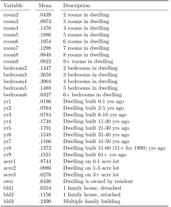
Table 3.1 Type Definitions . . . 42
Table 4.1 MSA Attribute Summary Statistics . . . 53
Table 4.2 Housing Hedonic: Variable Definitions . . . 55
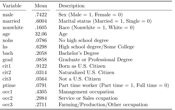
Table 4.3 Wage Hedonic: Variable Definitions . . . 56
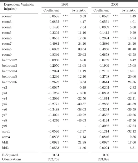
Table 4.4 MSA Housing Hedonic . . . 57
Table 4.5 Price and Index Summary Statistics . . . 58
Table 4.6 Income Regression: Summary of Coefficients for 229 MSAs . . . 59
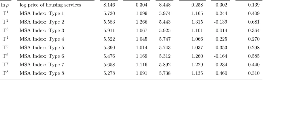
Table 5.1 Macro Sorting Parameters: Baseline Model . . . 73
Table 5.2 Macro Sorting Parameters: Restricted Index Model . . . 74
Table 5.3 Macro Sorting Parameters: Unrestricted Index Model . . . 75
Table 5.4 Macro Sorting Alternative Specific Constants . . . 76
Table 5.5 Second Stage Regression: Fixed Effects From Baseline Model . . . 77
Table 5.6 Second Stage Regression: Fixed Effects From Baseline Model With MC Interaction . . . 78
Table 5.7 Second Stage Regression: Fixed Effects From Restricted Model . . . 79
Table 5.8 Second Stage Regression: Fixed Effects From Restricted Model and MC Interaction . . . 80
Table 5.9 Second Stage Regression: Fixed Effects From Unrestricted Index Model . . 81
Table 5.10 Second Stage Regression: Fixed Effects From Unrestricted Model and MC Interaction . . . 82
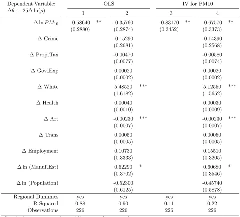
Table 5.11 MWTP for Reduction in PM10 Concentrations . . . 83
Table 5.12 Second Stage Regression: Fixed Effects From Restricted Model with Nor-malized Index and MC Interaction . . . 84
Table 5.13 Second Stage Regression: Fixed Effects From Unrestricted Model with Normalized Index and MC Interaction . . . 85
Table 5.14 Normalized Index: MWTP for Reduction in PM10 Concentrations . . . 86
Table 5.15 Second Stage Regression: Fixed Effects From Unrestricted Model with Heterogeneous Parameters on P M10 . . . 87
Table 5.16 MWTP for Reduction in PM10 Concentrations: Unrestricted Model with Heterogeneous Parameters on P M10 . . . 88
Table 5.17 Second Stage Regression: IV Regression, Pollution Variable = ln(110 -PM10) . . . 89
Table 5.18 Second Stage Regression: IV Regression, Quadratic in PM10 . . . 90
Table 5.19 AlternativeP M10Specifications: MWTP for Reduction in PM10 Concen-trations . . . 91
Table 7.1 Lowest COL Index (w/ MC), 1990 . . . 125
Table 7.4 Highest COL Index (w/ MC), 2000 . . . 128
Table 7.5 Lowest COL Index, 1990 . . . 129
Table 7.6 Highest COL Index, 1990 . . . 130
Table 7.7 Lowest COL Index, 2000 . . . 131
Table 7.8 Highest COL Index, 2000 . . . 132
Table 7.9 Regression of COL Index on Price of Housing Services, lnρY . . . 133
Table 7.10 Regression of COL Index on lnP M10 . . . 133
Table 7.11 Inequality as Measured by the Gini Coefficient . . . 134
Table 7.12 Inequality as Measured by the Gini Coefficient (Include MC in Expenditure Functions) . . . 135
Table 7.13 General Equilibrium Compensating Surplus . . . 136
Table 7.14 Gini Coefficient: Post-Simulation Equilibrium . . . 137
LIST OF FIGURES
Figure 4.1 Histogram of P M10 Concentrations: 1990 . . . 54
Figure 4.2 Histogram of P M10 Concentrations: 2000 . . . 54
Figure 6.1 The Lorenz Curve . . . 105
Chapter 1
Introduction
Residential sorting models have become prevalent in urban and environmental economics as a
tool for nonmarket valuation. Values for location-specific amenities are obtained by observing
residential location decisions in which households make tradeoffs between wage earnings, home
prices and environmental and other local public goods. The structural nature of these models
makes them convenient and powerful for estimating household preference parameters and
con-ducting counterfactual welfare analysis. This capability does not come for free, however, since
numerous assumption are necessary for implementation. Among these are the spatial scale of
analysis and the definition of choice alternatives. The first part of this dissertation focuses
on overcoming the limitations of current residential sorting models, particularly as they relate
to the choice set imposed on the consumer. In addition to contributions to the structure and
estimation of sorting models, I examine the empirical implications for non-market valuation.
The second part explores an application of the model related to spatially explicit measures
of the cost of living. The approach taken to develop such COL indices offers an alternative
to the current quality of life literature and an arguably more pertinent characterization of
access to public amenities. The analysis also focuses on the distribution of such welfare across
the population. Income inequality has gained considerable attention in recent years and has
the discussion may benefit from a better definition of the unequally distributed asset. Public
policy may be less concerned with the distribution of income than with the distribution of a
broader measure of the standard of living. Distributional issues relate to the fairness of the
public provision of goods, such as whether public amenities disproportionately benefit particular
income groups. This is an obvious policy concern that requires empirical evidence.
Sorting models to date have operated at the macro level (e.g. Bayer et al. (2009)) or micro
level (e.g. Klaiber and Phaneuf (2010)). The former typically involves modeling the decision of
which city to locate to from a collection of metropolitan areas across the country, while the latter
focuses on which neighborhood a household selects within a city. Usually the scale of analysis is
determined by the objectives of the study, in that amenity levels can vary at the local, regional,
or national scale. Regardless of the scale, all sorting models in the current literature analyze
a single choice from a single set of alternatives. Although this is computationally convenient,
it ignores a stylized reality. In particular, household location choices tend to be two tiered. A
large scale choice of which region or metropolitan area in which to reside is followed by a smaller
scale neighborhood choice. The first of these may depend on labor market considerations and
regionally varying amenities such as climate and certain types of air quality. The second may
depend on local amenities such as proximity to open space and school quality. These choices
can interact in a variety of ways, in that the macro level choice might depend on the portfolio
of micro-level amenities provided by the area.
I develop a sorting model that formally reflects two levels of choice. I show how an
as-sumption of two-stage budgeting, which is inherent in the structure typically used for empirical
analysis, allows me to separately analyze the two choices and then link them in a single model.
More specifically, the micro level choice sets and choice behavior are aggregated into a quality
adjusted price index for the macro level decision. This provides a structurally consistent means
of considering the role of both regional and local environmental variables in household decisions.
I propose a feasible empirical version of this model at the macro level, which can be estimated
Importantly, though the approach accounts for local public goods, I do not need to measure
amenities at the local level across the macro landscape.
I demonstrate these ideas with a model that focuses on valuing air quality. If one considers
variation in pollution across (but not within) metropolitan areas, valuation is possible through
the macro sorting process. However, ignoring the impact of variation in micro-level amenities
may confound identification of willingness to pay for macro-level amenities. To examine this
I compare estimates of marginal willingness to pay for air quality obtained from the model
with estimates obtained from a conventional macro sorting model. Empirical results show that
this additional margin of sorting has considerable impacts on valuation of air pollution. Using
a two-stage approach to residential sorting, the marginal willingness to pay for reductions in
particulate matter (P M10) increases upwards of 100%. In modeling the second stage of sorting,
I identify an additional set of amenities over which individuals optimize and make tradeoffs
with pollution. Note that the increase in willingness to pay is an empirical finding based on
the relationship between air pollution and the set of local amenities, rather than a general
theoretical result.
An application of the developed model examines a measure of welfare that reflects income,
market prices, and the value of public goods. The structural approach allows for calculation of
a true cost of living (COL) index that varies across space, which can then be used to construct
a broad measure of standard of living. Development of true COL indices also allows for
calcu-lation of an adjusted income measure and precise characterization of the dispersion of welfare.
With this, I measure the degree to which access to public amenities disproportionately benefits
households based on their income.
Furthermore, I simulate federal policies in the form of exogenous changes in air pollution
across different sets of locations to examine the distributional effects of federal public good
provision. In response to policy that alters the level of some public good, individuals
re-optimize and may move to new locations when one considers general equilibrium price effects.
Partial equilibrium welfare analysis will fail to measure the gain or loss from any non-marginal
changes in spatially delineated site attributes, as consumer optimization will result in individuals
reallocating their housing and public good consumption. Thus, any examination of exogenous
shocks must allow individuals to re-sort among residential locations. The residential sorting
model offers a means of estimating the underlying process of the residential choice, rather than
simply characterizing the equilibrium outcome. Knowledge of the sorting process allows for
counterfactual analysis, in which a re-sorting due to public policy can be simulated. Then, one
can ask, for example, whether individuals with already high levels of quality adjusted income
are receiving a disproportionately high level of the welfare gain. This reveals the regressive or
progressive effect of public good provision.
In general, explicitly accounting for public goods leads to a distribution of adjusted income
that has a wider spread than that of pure monetary income. This implies that households
with less income tend to face higher costs of living, determined by an inferior set of public
goods relative to housing prices paid to obtain such goods. Such a widening of the distribution
is a function of costly migration and the joint distribution of initial household locations and
set of public goods. Simulations show that the distributional impacts of federal policy, in the
form of pollution reductions, are highly dependent on the location in which they are targeted.
Furthermore, general equilibrium re-sorting among locations has significant impacts on the
distribution of benefits from policy, as households compete in the housing market to obtain
access to public good improvements.
This dissertation proceeds as follows. Chapter 2 reviews the sorting model literature,
in-cluding its development, empirical applications, and shortcomings. In Chapter 3, I discuss the
theoretical foundation of residential sorting models and develop a theoretical and empirical
model that incorporates the two-stage location choice introduced above. Data and estimation
results are presented in Chapters 4 and 5 respectively. The final two chapters concentrate on
cost of living indices and adjusted income. Chapter 6 includes a literature review related to cost
constructing a metric for comparing distributions. Chapter 7 then presents calculated indices,
Chapter 2
Literature Review
2.1
Residential Sorting Models
Residential sorting models offer an approach to nonmarket valuation based on the implicit
purchase of location specific amenities and public goods. When an individual chooses a location
in which to live, she also chooses the amenities available at that site. The residential location
choice is based on a utility maximizing framework in which individuals choose the location that
offers their optimal bundle of market and nonmarket goods. The resulting equilibrium reveals
information about the population’s preferences and willingness to pay for public goods.
The structural nature of empirical sorting models is a key advantage over hedonic estimation
(Roback, 1982). While a hedonic price function uses the observed equilibrium to estimate the
marginal price of a particular good, sorting models estimate the underlying preference structure
that determines the observed equilibrium. Therefore, while some applications focus on the
willingness to pay for particular goods such as air quality (Bayer et al., 2009) or open space
(Klaiber and Phaneuf, 2010), some conduct counterfactual analyses for policy evaluation. These
counterfactuals can be used to estimate welfare effects in a general equilibrium context in which
individuals re-sort among locations. Given an underlying preference structure, sorting models
approaches (Kahn (1995), Banzhaf (2005)). Furthermore, by matching equilibrium predictions
to observed outcomes, one can empirically test models of spatial theory.
Sorting models typically fall into one of three general theoretical frameworks; 1) an
equilib-rium stratification framework (Epple and Platt (1998) and Epple and Sieg (1999)), 2) a random
utility model (Bayer et al. (2005)), and 3) a general equilibrium model with an amenity
pro-duction function (Ferreyra (2007)). Though the intuition behind the models is similar, they
differ significantly in their analytical approaches. This leads to empirical applications that vary
regarding the choice set, the structure of the housing market, the characterization of
heteroge-neous preferences, and geographic mobility costs.
2.1.1 Development of Literature
The foundation for residential sorting can be attributed to Tiebout (1956). The author argues
that the level of public expenditures at the local level are efficiently allocated through the
movement of individuals. An individual’s decision to move or remain in her current location
“replaces the usual market test of willingness to buy a good.” Thus preferences for local public
goods are reflected in the equilibrium location decision. Advances in computing power and data
availability have led to numerous empirical studies of this mechanism.
The degree to which location decisions reveal demands identical to those of a market
sit-uation rests on the amount of information available to the consumer, the size and variation
of the choice set, and the cost of mobility. Imperative in a model of geographic choice,
mo-bility constraints hinder the efficient allocation of public goods. This problem is approached
empirically in Bayer et al. (2009). Tiebout’s discussion also abstracts from the labor market,
assuming that employment opportunities do not impact location decisions. Empirical analyses
rely on a related literature that grew from a labor sorting model proposed in Roy (1951), which
seeks to model potential income and characterize the relationship between the labor market
and the residential location choice problem. Another assumption of Tiebout’s analysis is the
of a particular community provide no utility for members of neighboring communities. Such
external spillovers have been largely ignored in the literature. Finally, current sorting models
have sought to address additional oversights of the original model, such as unobserved and
endogenous attributes, estimation of location prices, and the existence of a spatial equilibrium.
Banzhaf and Walsh (2008) use a reduced form approach as a direct test of residential
sorting. Given that individuals choose the location with the optimal allocation of goods and
prices, an exogenous change in a location’s attributes should result in population changes.
The authors use a difference-in-difference model to study the impact of the siting of polluting
firms on a location’s population and population composition. Empirical results demonstrate
population declines in response to increased toxic emissions. In addition, the authors note the
existence of income effects in which exogenous increases in a normal public good attract higher
income households to a neighborhood. In general, this study shows that migration patterns are
consistent with the idea that individuals move in response to location attributes and prices,
offering support for the type of sorting discussed in Tiebout (1956).
A similar type of sorting exists in the labor market, in which individuals choose an optimal
job. Roy (1951) describes an economy with two occupations in which each individual is endowed
with a certain skill level for each. The resulting distribution of wages is a general equilibrium
outcome related to the distribution of skills. When labor markets are geographically defined,
another dimension is added to the labor market choice. The relationship between skills and
preferences for location attributes makes separate identification of them difficult. Empirically,
the researcher must distinguish between an individual receiving lower wages due to her skill
level versus receiving lower wages due to a compensating differential on location specific public
goods.
As potential income levels are important location choice attributes, prediction of potential
wages becomes a necessary component of sorting models. Self-selection in the labor market,
however, confounds such prediction. Thus, significant research has been done to characterize
Bayer et al. 2009). A related literature demonstrates how residential sorting can be used to
identify potential wages in an economy with labor market sorting (Bayer et al., 2011).
Given a theoretical foundation and empirical evidence for location sorting, additional
re-search explores the existence and uniqueness of an equilibrium. Epple and Platt (1998) describe
the necessary conditions for a sorting equilibrium to exist in a model of consumers that differ in
income and preferences and locations that differ in tax rates and the level of public goods.
Equi-librium is defined as the allocation of each individual to a single location such that consumers
maximize utility, the housing market clears, local government budgets balance, and taxes and
government spending are decided through majority vote. Existence relies on a preference
struc-ture in which there are sets of income-preference combinations that make consumers indifferent
between two neighborhoods and in which consumers smoothly tradeoff between consumption
of housing and public goods so that higher income individuals substitute towards housing.
An alternative proof of a sorting equilibrium is given in Bayer et al. (2005). The authors
prove the existence of a unique housing price vector that clears the market when utility is a
decreasing, linear function of the price of housing. Furthermore, they also show the existence of
an equilibrium in the presence of preferences for the endogenously determined sociodemographic
composition of each neighborhood.
Under the assumption that individuals do optimally sort, many studies have taken a
struc-tural approach to examine individuals’ preferences for public goods. Epple and Platt (1998)
develop a vertical model of residential sorting in which households are defined based on their
level of income and a single preference parameter. Although variance in this preference
pa-rameter conveys heterogeneity in preferences for housing versus public goods, it does not allow
for heterogeneity in preferences for individual public goods. Thus, all households agree on
a ranking of communities by each location’s aggregate level of public goods. It is assumed
that each household has a Cobb-Douglass utility function that includes housing and numeraire
consumption, while public goods linearly enter the budget constraint. This class of models is
indiffer-ent between two communities. Then, these conditions implicity define the set of income and
preference parameters for which a household would optimally choose any given community. A
key aspect of such models is that they rely only on aggregate location data, rather than the
choice and attributes of individual households.
A theoretical model shows that neighborhood sorting leads to an equilibrium in which
stratification occurs based on income and preferences. This contrasts with previous results
that predicted perfect income stratification. The authors also estimate income and preference
distributions to calibrate and simulate a sorting model. Simulation of a two location model
demonstrates the relationship between heterogeneous preferences and the lack of pure income
sorting. In particular, when the variance of the preference parameter decreases, implyinging
less preference heterogeneity, equilibrium approaches the case of perfect income stratification.
Epple and Sieg (1999) use an identical model to empirically estimate preferences for public
goods. The model is estimated using aggregate community data from 92 municipalities in the
Boston, MA metropolitan area. The cost of housing is estimated using structural assumptions
of the model that define a relationship between income, observed housing expenditures, and the
cost of housing that is necessary for the model. Income is ignored as part of the location choice.
The authors use the observed income and population distributions across locations to estimate
structural parameters of these distributions as well as parameters in the utility function.
Fol-lowing identification of these parameters, estimation of public good consumption is based on
the role of public goods in the boundary indifference conditions implied by stratification. The
boundary indifference conditions allow aggregate public good levels to be written as a function
of location populations and housing prices. Due to the nature of preference heterogeneity
ag-gregate public good levels can be decomposed into levels of individual public goods to obtain
values for public goods. A simple linear specification includes the crime rate and per capital
expenditures on education. However, the value of location amenities in this model must be
interpreted as a monetary tradeoff between public goods, rather than a marginal price.
sorting model to examine changes in ozone concentrations. The model follows that of Epple
and Sieg (1999) but develops a new estimation procedure. More specifically, the study uses
instrumental variables to increase the number of orthogonality conditions and estimate all
parameters in a single stage. The model is estimated on school districts in the Los Angeles
metropolitan area. Measuring the welfare impact of air quality improvement, empirical results
show that general equilibrium benefits are substantially different from estimates obtained in
partial equilibrium analysis.
The restriction on preferences in the previous papers is relaxed in Kuminoff (2008), which
develops a horizontal sorting model that allows households to have heterogeneous preferences
for individual public goods. Another important contribution here is the inclusion of the labor
market. Each location offers an individual a wage that depends on the product of some average
wage and an individual skill parameter. This skill parameter is estimated simultaneously with
other model parameters. The analysis focuses on 268 neighborhood-labor market combinations
in the San Francisco-Sacramento CMSA, using individual housing transaction data. Location
amenities include air quality and school quality, proxied by ozone and a composite index of test
scores, respectively. Estimates for the MWTP for air quality are significantly higher than those
obtained from hedonic studies. In addition, preference heterogeneity and an endogenous labor
market decision increase estimates on MWTP.
A second class of sorting models builds on a random utility model (RUM) framework,
out-lined in Bayer et al. (2005). The study specifies an indirect utility function that includes housing
and neighborhood characteristics, housing prices, work commute distance, unobserved
neighbor-hood characteristics, and neighborneighbor-hood level sociodemographic variables that are determined in
equilibrium. Heterogeneous preferences are easily modeled by interacting preference parameters
with an individual’s income, education, race, employment status and household composition.
This framework defines a horizontal model, in which preferences are defined over the attributes
of a location, rather than over a location specific index. An important contribution is its
The empirical analysis uses confidential census data that identifies a household in its census
block within the San Franciso MSA. Given this definition of the choice set, utility maximization
is restricted to choosing from a set of neighborhoods within the MSA. Neighborhood variables
include school quality, elevation, population density, crime, and sociodemographics. Estimation
follows the two step empirical strategy of Berry et al. (1995), in which the first stage estimates
location fixed effects and the second stage decomposes fixed effects based on location attributes.
This approach has become a common strategy in estimating sorting models. The authors then
use the parameterized model to conduct a simulation in which the income distribution is altered.
Simulation involves an iterative process that converges to a price vector and sociodemographic
composition for each location. The results of the counterfactual analysis demonstrate general
equilibrium price changes and partial stratification consistent with theoretical predictions of
residential sorting.
Bayer and Timmins (2005) further explore equilibrium in the context of RUM-style sorting
models. In particular, they outline the conditions under which a unique equilibrium is obtained
in the presence of local spillovers. This is akin to the existence of population as an
endoge-nously determined attribute. When individuals are averse to the endogenous share variable
(congestion), the corresponding coefficient is negative and a unique equilibrium is guaranteed.
However, in the case of preferences for endogenous shares (agglomeration), uniqueness is only
guaranteed if the effect is less than some value. This value is analytically shown to depend on
other components of the model, including site attributes and the distribution of preferences.
Simulation demonstrates that the threshold value for uniqueness increases with the number of
alternative choices, heterogeneity in preferences, and variation in the utility contribution of
ex-ogenous site attributes. Additional analytical results, however, show that multiple equilibrium
may arise when local spillover effects are preference-specific (i.e. particular types of individuals
have preferences for living with similar types).
A general theoretical result in sorting models is that utility is equalized across locations
would have incentive to relocate, driving up prices through increased demand for housing. Since
utilities are equal, observed housing price and wage differentials reveal the aggregate impact
of public goods. Kahn (1995) takes advantage of this property to rank the aggregate level
of location amenities across cities using sorting equilibrium, rather than relying on hedonic
methods in which it is necessary to observe amenity levels.
Bayer et al. (2009) use an application to air quality to empirically compare valuation in
sorting models and hedonic estimation. The most important difference between the two
ap-proaches is that sorting models can incorporate the moving costs an individual faces in choosing
a residential location. The hedonic model assumes free mobility, which causes all local amenity
values to be reflected in wage and housing price differences. The authors use a structural
framework to derive an indirect utility function similar to that of Bayer et al. (2005), but focus
on MSA level attributes, with a choice set that includes only MSAs across the country rather
than neighborhoods within any particular MSA. The extension here is that Bayer et al. (2009)
include dummy variables that indicate an individual leaving his birth state, birth region, and
birth macro-region, respectively, to capture money and non-money moving costs. For
compar-ison, a conventional hedonic approach uses wage and housing regressions to obtain estimates
of the marginal willingness to pay (MWTP) for air quality. Empirical results show significant
differences in MWTP for air quality between the two approaches. These results emphasize the
importance of mobility constraints in location decisions, particularly when modeling a macro
level choice.
Focusing on open space as a location amenity, Klaiber and Phaneuf (2010) estimate a
model of sorting among small neighborhoods in a single city. Using extremely fine location and
attribute data, this paper obtains values for environmental amenities at a very disaggregated
level. Similar to Bayer et al. (2005) an advantage of the model is its high spatial definition. Of
course, such an analysis is difficult when one wants to consider multiple cities. In addition, a
rich characterization of heterogeneous preferences demonstrates variance in MWTP estimates
While many empirical studies in the sorting literature are concerned primarily with
esti-mating the marginal willingness to pay for some public good, sorting models offer a means
of computing policy outcomes in a general equilibrium framework. This involves simulating
some change in exogenous variables, followed by an iteration in which individuals maximize
their utility function and housing prices and endogenous variables converge to equilibrium.
Tra (2010) considers a non-marginal change in air quality. In particular, the paper first
esti-mates a residential sorting model across 87 public use micro areas (PUMAs) in the Los Angeles
metropolitan area. The analysis then uses these estimates to simulate a new location
equilib-rium in which the level of air pollution is consistent with improvements due to the 1990 Clean
Air Act Amendments and all other attributes are unchanged. This approach offers a direct
means of calculating welfare impacts of a specific policy. Empirical results display a substantial
difference between partial and general equilibrium effects when public good adjustments are
non-marginal. Timmins and Murdock (2007) analyze the effect of removing one site from the
choice set, using a model with local spillovers. Their application focuses on recreational fishing
areas in the state of Wisconsin. Rather than a welfare loss equal to the implicit value of that
site’s amenities, individuals re-sort to other sites. Therefore, the model incorporates the added
congestion effect into general equilibrium impacts.
2.1.2 Issues in Applications
A number of questions arise in specifying and estimating sorting models. Among these are
definitions of the choice set, estimating location prices, predicting potential income, controlling
for endogenous variables, and accounting for costly migration. A large body of research, as
discussed above, has addressed many of these aspects, though significant issues remain.
Sorting models imply a location choice from a fixed set of alternatives. The choice set may
include cities within a country (Kahn (1995), Bayer et al. (2009)), neighborhoods within a
city (Bayer et al. (2005), Klaiber and Phaneuf (2010)), or one of many other designations. In
choice set, though the true choice behavior of households likely determines the set of amenities
for which valuation using sorting models is valid. In addition, empirical applications so far
have focused on a single location choice. For example, the model in Bayer et al. (2005) allows
households to select from a number of neighborhoods within Los Angeles but restricts them
to staying in Los Angeles rather than leaving the city. It also fails to distinguish those that
came from another city from those that originated from within Los Angeles. Similarly, Bayer
et al. (2009) specify a choice among cities but ignore the variance in neighborhood location
choices among all of the households that chose to live in a particular city. For these reasons,
development of sorting models may benefit from a integrated choice model that incorporates
the location decision at different levels.
Another aspect of the choice set that deserves attention is the affordability of alternatives.
Many of the RUM-style sorting models assume that all households can afford any home. Tra
(2010), however, slightly adjusts the indirect utility function to force the choice probability to
zero as the cost of housing in a location approaches an individual’s income. The stratification
models based on Epple and Platt (1998) only assume that a household can purchase a subset
of homes in their chosen neighborhood and in the next most expensive community.
Housing prices are typically estimated separate from the sorting model. Epple and Sieg
(1999) estimate prices by combining observed income data and housing demand obtained from
the model structure, though this is required due to data constraints. The conventional approach
is to estimate housing prices in a hedonic framework that removes the impact of structural
attributes, such as the number of rooms or age of the house. The results are comparable prices
for a homogeneous housing good. However, this requires somewhat strict linear functional form
assumptions and restricts the value of structural amenities to be constant across locations. Sieg
et al. (2002) show that obtaining housing prices from hedonic regressions is consistent with
sorting equilibrium when utility is separable in housing. The accuracy of housing price indices
are tested against theoretical predictions of location sorting, though predictions are based on a
Potential income is a necessary variable to describe the attributes of each location in the
choice model. A related literature involves the role of income in residential sorting models.
Roy (1951) discusses the means by which individuals self select into different occupations and
examines the resulting observed distribution of earnings as it relates to the underlying
distri-bution of skills in an economy. Given data on the distridistri-bution of wages in different markets,
Heckman and Honore (1990) show that it is possible to identify the distribution of potential
income across markets without any distributional assumptions.
Given the complexity of identifying potential wages, Dahl (2002) offers a simplified
ap-proach using nonparametric controls. The fundamental problem in identifying potential wages
is that unobserved factors that contribute to an individual’s choice of a labor market may be
correlated with individual attributes that determine wages. Therefore, coefficients in a linear
wage regression are biased and generate problems for predicting wages. The strategy in Dahl
(2002) is based on the notion that information related to labor market unobservables is
con-tained in migration pattern choice probabilities. To simplify further, it is assumed that only
optimal migration choice probabilities matter. Such probabilities then serve as controls for Roy
sorting in a linear wage regression. Bayer et al. (2009) employ this approach in the context of
a residential sorting model. Bayer et al. (2011) use location sorting as a means of estimating
a model of Roy sorting. They exploit a non-pecuniary component of utility that varies across
locations to identify potential wages in different labor markets. Though the objective of the
paper is to estimate the wage distribution, no further research has sought to simultaneously
estimate amenity prices.
Location price and sociodemographic attributes are naturally endogenous in a model of
location choice. Properties of sorting equilibrium, however, offer possibilities for
construct-ing instruments. Sieg et al. (2004) propose an instrument for the level of public goods based
on community rank. The validity of this instrument follows from unobserved community
at-tributes being small enough to affect only prices and equilibrium sorting, but not the rank of
Klaiber and Phaneuf (2010) exploit the fact that demand for housing in a location is likely
impacted by prices in other locations through general equilibrium effects. Therefore, an
instru-ment is developed using neighborhood and housing attributes from surround communities. The
general equilibrium argument to justify correlation is also used in Bayer and Timmins (2007),
which discusses an approach to instrument for local spillover effects. Since location shares are
endogenously determined, the authors predict shares using only exogenous attributes from
sur-round alternatives. This approach is then applied to a model of recreation fishing decisions
in Timmins and Murdock (2007). In these cases, the power of the instrument is derived from
variation in different regions of the spatial landscape. An alternative means of dealing with
endogenous prices is to appeal to the structure of the model. Bayer et al. (2009) derive an
expression for the price coefficient that involves the demand for housing services. Housing
ex-penditures are then calculated from observed data and the impact of price is simply a calculated
value rather than a component to be estimated.
Second stage estimation in RUM sorting models is typically in the form of a linear
regres-sion on location attributes. Thus, in the case of endogeneity problems driven by unobserved
attributes, estimation can follow a more conventional instrumental variable technique. Bayer
et al. (2005) use a boundary discontinutiy approach developed by Black (1999) to instrument
for school quality, in which it is assumed that while school quality changes in a discrete manner
across district lines, unobservables change in a continuously. Though it depends on finding
ap-propriate instruments, a second stage instrumental variable regression can be applied to most
sorting applications.
Finally, the integration of moving costs has proved to be a significant aspect of residential
sorting models. As mentioned above, Bayer et al. (2009) control for moving costs, but in a
very simplistic manner. Moving costs in their paper are constructed to control for the cost
of being away from one’s birth place, but there is no control for the qualitatively, and likely
quantitatively, different cost of moving from a second to a third location. In addition, no
that focus on smaller scale sorting, such as within cities, generally ignore moving costs based
on the short distance of the move. However, it may be a bold assumption in imposing zero
costs to reoptimize and purchase a new home, when one considers transaction cost as a type of
moving cost.
Given the need for additional research to address limitations of residential sorting models,
the next chapter will focus primarily on examining the role of the choice set and the geographic
scale of the location decision. In particular, I develop a single horizontal sorting model that
encompasses macro sorting across cities (Bayer et al., 2009) and micro sorting across
Chapter 3
Theoretical Model
This section outlines theory related to constructing a multi-level residential sorting model. The
first subsection describes a sorting model in its most general form. The second subsection
focuses on two-stage budgeting. In particular, I provide conditions under which a two-stage
budgeting approach is consistent with utility maximization, and relate these conditions to the
sorting context. Lastly, I examine a sorting model based specifically on a two-stage budgeting
process.
3.1
Generalized Horizontal Sorting Model
Residential sorting models are based on random utility maximization (RUM) models in which
individuals choose their location to maximize well-being. Utility is comprised of a deterministic
portion that is observed by the analyst and a random portion that is known only to the decision
maker. Sorting models rest on the notion that when an individual purchases a house, she
simultaneously chooses all the attributes that accompany that house and its location. Therefore,
the deterministic component of utility includes variables that describe structural characteristics
of the house, location-specific public goods and amenities, and the household’s location-specific
income potential. The random component is an idiosyncratic preference shock that is specific
residential choice as a preface to the specific functional forms and structural assumptions to be
discussed later.
Suppose an individual or household i chooses a locationj to maximize utility, where each
location j = 1, ..., J offers a bundle of location specific amenities and defines a distinct labor
market. At the intensive margin the household optimizes over consumption of a numeraire good
C and continuous housing servicesH, subject to a budget constraint. Specifically, individuals
solve a maximization problem of the form
max
j=1,...,J
max
C,H Uij =U(C, H, Xj, ξj, ηij;β
i) s.t. C+ρ
jH=Iij
, (3.1)
where Uij is the location j specific utility level, and Xj is a vector of observable location
attributes that contains public goods such as air quality, school quality, and cultural amenities.
Unobserved variables are decomposed intoξj, which is constant for all people in a location, and
ηij, which is an individual-level random idiosyncrasy. Income for household i in location j is
denoted by Iij where the location subscript implies earnings can depend on the labor market
the household selects. A vector of preference parameters is denoted byβi, where the superscript
indicates that preferences can vary across individuals.
In equation (3.1) the price of all non-housing market goods is normalized to one for all
locations. The amountρjHis expenditures on housing. By writing expenditures in this form, I
assume there is a continuous housing services index, where the choice of the bundle of structural
characteristics of a property is reflected in the level ofH. ThusH can be viewed as the output
from a production function that maps a multiple dimension vector of property characteristics
to a continuous, ordinal index. I assume this production function is constant for all locations.
Under this assumptionρj is the price of a single unit of housing services in locationj.
The inner optimization of (3.1) results in conditional Marshallian demands for consumption
and housing services C(Iij, Xj, ρj, ξj, ηij;βi) andH(Iij, Xj, ρj, ξj, ηij;βi), respectively.
condi-tional indirect utility function
Wij =W(Iij, Xj, ρj, ξj, ηij;βi), j= 1, ..., J (3.2)
To make estimation feasible additional assumptions are necessary concerning the
idiosyn-cratic utility component, ηij. Following convention, we assume the indirect utility function is
multiplicative inηij, so that the natural log of utility can be written
lnW(Iij, Xj, ρj, ξj, ηij;βi) = lnV(Iij, Xj, ρj, ξj;βi) +ηij, j= 1, ..., J (3.3)
The standard choice rule implies that households are observed in a location only if that
location generates higher utility than all others. This choice is deterministic from the
house-hold’s perspective, but stochastic from an observer’s perspective due to the random variable
ηij. By knowing the distribution of ηij we can derive the probability of observing household i
in locationj as
P rij =P r(lnVij +ηij ≥lnViq+ηiq ∀q 6=j). (3.4)
Following Bayer et al. (2005), a sorting equilibrium exists when the housing market clears
and each household chooses its optimal location, given the decisions of all other households. If
Vij is a decreasing, linear function of price andηis drawn from a continuous distribution, Bayer
et al. (2005) show that there exists a vector of housing prices that leads to a sorting equilibrium.
Such an equilibrium implies that all households are in their optimal location, given the decision
of all other households.
The assumed distribution ofη determines the form of the right hand side of equation (3.4)
and thus, the class of discrete choice model. Issues concerning endogenous attributes,
unob-served variables, and estimation will be discussed later in the context of specific functional
3.2
Two-Stage Budgeting
A defining characteristic of the model described above is that the choice is limited to a single
element from a given set of alternatives. In the context of a sorting model, this implies
house-holds select a particular city (in macro level models), a neighborhood within a city (in micro
level models), or from a large choice set consisting of all possible combinations of cities and
neighborhoods. The latter tends to be empirically infeasible due to the large choice set and
substantial data needed. Furthermore, individual macro and micro sorting models ignore the
stylized reality that household location choices tend to be two tiered. First a particular labor
market is selected, which tends to correspond to a metropolitan area; conditional on this a
neighborhood is selected based on local housing prices and local public goods. In what follows,
I examine how an assumption of two-stage budgeting can be used to specify an empirically
tractable model that is consistent with this two tiered intuition.
In consumer choice theory, two-stage budgeting postulates a budget allocation process in
which expenditures are assigned to broad groups of consumption categories and then allocated
to individual goods within each group, conditional on group-level expenditures. The practical
benefit of such a framework is that it allows the researcher to separately analyze the two stages,
where group level expenditures depend on group price indices rather than individual prices, and
within group allocations depend on individual prices and group (rather than total) expenditures.
Of course, this pattern of consumption behavior does not always hold. Two-stage
budget-ing depends on assumptions regardbudget-ing functional forms of the underlybudget-ing optimization problem.
As described by Blackorby and Russell (1997), two-stage budgeting is consistent with utility
maximization when both price aggregation and decentralisability are satisfied, corresponding
to optimal behavior in two stages. In the first stage, price aggregation implies an optimization
problem that depends on group-level price indices rather than individual product prices.
Con-sumers optimally allocate expenditures to broad commodity groups based on price aggregates
determined expenditures on the group. When price aggregation and decentralisability are
sat-isfied, the consumer’s two-stage optimization problem is identical to optimizing over all goods.
The following subsections define conditions under which these concepts hold.
3.2.1 Price Aggregation
Partition the set of allN goods intoGgroups,G≤N, with the vector of prices of goods in group
g denoted aspg. Define price indices Λg that aggregate prices of the individual commodities of
each group to a single group index. Also, define allocation functions Θg that map all prices and
income into optimal group expenditures. Strong price aggregation is defined as the existence
of linearly homogeneous index functions for each group,
Λg(pg), g= 1, ...G (3.5)
and linearly homogeneous expenditure allocation functions of the form,
Eg = Θg I,Λ1(p1), ...,ΛG(pG)
g= 1, .., G, (3.6)
whereI is total expenditure andEg is optimal expenditure on groupg. The above makes clear
that groupgexpenditures can be determined with knowledge of only income and group indices.
Conditions under which price aggregation holds are most evident from the expenditure
function. If the expenditure function can be written as
E(p, u) =E k(p, u),Λ1(p1), ...,ΛG(pG), (3.7)
where k(·) is homogeneous of degree zero inp and Λg(pg) are homothetic for all g, then price
aggregation is satisfied (Blackorby and Russell, 1997). Here, the expenditure function depends
on price indices and a homogeneous function of all prices and utility. This ensures optimality
3.2.2 Decentralisability
Corresponding to the second stage of budgeting, strong decentralisability (for the remainder of
this chapter, strong decentralisability is implied when decentralisability is discussed) requires
that goods within a single group can be properly allocated based only on group expenditures
and prices of the commodities within the group. Denote the vector of demand for goods in group
g as dg(I, p). Then, define the function Φg that maps income and prices within a particular
group into a vector of demand. Decentralisability holds if demands can be expressed as
dg(I, p) = Φg(Eg, pg) ∀g= 1, ..., G. (3.8)
Thus, demand for commodities within a particular group can be determined from group
expen-ditures and prices of goods in that group. Prices of goods in other groups will affect demand
for goods in gonly through their impact on expenditure allocated to group g.
Denote qg as the consumption bundle of goods in group g. Decentralisability is satisfied
(Blackorby and Russell, 1997) when there exist subutility functions, Ug, and a continuous,
positive monotonic, and strictly quasi-concave separable utility function of the form
U(q) = U1(q1), ..., UG(qG). (3.9)
When utility is separable in in some partition of commodities, maximization can proceed over
subutility functions for different commodity groups. Together, equations (3.7) and (3.9) define
necessary and sufficient conditions for two-stage budgeting analysis (see Appendix A and B for
further discussion). Later, it will be shown that functional forms commonly used in sorting
3.3
Two-Stage Residential Sorting Model
When two-stage budgeting holds for the underlying preference structure of the sorting model,
the residential choice can be modeled in two stages. These stages are defined based on the
geographic level at which the separable commodity groups vary. The conventional residential
sorting model links each house to one specific geographic entity. In the current study each
house corresponds to two locations, where one location encompasses the other. In the empirical
application, I use census tracts and metropolitan statistical areas (MSA), which are comprised
of multiple tracts, as the two levels, though other divisions are possible. In general this type of
differential spatial resolution implies that some public amenities vary at a micro level (across
census tracts) and others vary only at a macro level (across MSAs). In this case, the two-stage
budgeting process is analogous to a sequential location choice that proceeds at two geographic
levels. One aggregate commodity group is MSA level spending on housing, which is then divided
between housing services and local location amenities in the second stage.
To examine this formally I rewrite the utility maximization problem for individual i in
neighborhood (census tract) j of MSAm as
max
C,H Uijm =U(C, H, Xjm, Ym, ξjm, ζm, ηijm;β
i) (3.10)
s.t. C+pjmH ≤Iim. (3.11)
The additional notation in (3.10) and (3.11) is defined as follows. There are now two types
of location specific attributes entering preferences. The vector Xjm refers to observed
charac-teristics specific to tract j in MSA m, while the vector Ym refers to observed characteristics
that vary only over MSAs. The difference between MSA and tract characteristics is based on
the extent of variability in location amenities. Any amenity that is constant across tracts in
an MSA is considered an MSA amenity that is captured byYm, and the vector Xjm captures
tract-level deviations from MSA levels. Likewise the scalars ξjm and ζm refer to tract-varying
given by ηijm. The scalarpjm is the price of housing services in a particular tract, conditional
on a particular MSA, and it varies across the entire micro and macro landscape based on
lo-cal spatial characteristics. This price can be further decomposed into an MSA and a tract
component
pjm=ρXmρYjm, (3.12)
where ρYm varies only across MSAs and ρXjm varies with tracts in each MSA. The component
that varies at the MSA level can be interpreted as a base MSA price, while the component
that varies at the tract level can be interpreted as a price adjustment arising from the variation
in tract-level amenities. Finally, based on the notion that an MSA is a single labor market,
income varies only across MSAs. These assumptions give rise to a conditional indirect utility
function of the form
Vijm=V(Iim, pjm, Ym, Xjm, ξjm, ζm, ηijm;βi), j= 1, ..., Jm, m= 1, ..., M, (3.13)
whereJm is the number of census tracts in MSAm.
A specific function form for equation (3.10) will ensure that two-stage budgeting holds. A
sufficient condition for two-stage budgeting is that the conditional indirect utility function can
be expressed as a function of price indices that correspond to consumption groups. I define
three consumption groups as general consumption C, the MSA-level public goods Y, and a
composite good Q. The latter group is an aggregate of tract-level public goodsX and housing
services H. If two-stage budgeting holds we can rewrite (3.13) as
where the idiosyncratic error term is divided into two components so that ηijm =ηij|m+ηim,
and Γijm(·) is a price index for individual i in tract j of MSA m. The index reflects the
aggregation of tract-level public goods, tract-level unobservables and housing services. Due to
the fixed quantity nature and implicit pricing of public goods, the index Γijm(·) includes levels
of the commodityXrather than the explicit price ofX. While the price index here corresponds
to the index Λg discussed earlier, notation has been changed for two reasons to avoid direct
comparison. First, more conventional price indices include the price of a good rather than the
level, as is the case for Γijm(·). Second, the subscriptj on each Γijm(·) illustrates that the index
summarizing tract level public goods and prices corresponds to an optimal decision regarding
tract choice; likewise the superscriptihighlights the role of preferences in the structure of the
price index.
Under certain conditions, the two-stage sorting model discussed above collapses to a
single-stage MSA sorting model. When all neighborhoods in an MSA are identical, the second single-stage
of sorting becomes irrelevant since all variaiton occurs at the MSA level. In such a situation,
there should be no variation in price across tracts. THus, ρX
jm = 1 for all tracts in the MSA
so that each tract has a price described only by the MSA portion ρYm. Given this special case
forρXjm, it is evident that the price function in equation (3.12) becomes identical to that of the
more conventional model in equation (3.1).
To summarize, an individual chooses from among a set of MSAs that each offer a fixed
bundle of income, MSA-level public goods, and a composite good. The composite good consists
of housing services and tract-level public goods, where each tract offers a different bundle of
public goods and housing prices. The choice of an MSA is analogous to choosing optimal
expenditures on the broad groups of commodities, including housing, without choosing the
exact consumption of housing services and local public goods. In other words, an individual
decides on an MSA without yet determining a particular tract. The choice of a tract is then
analogous to choosing the bundle that optimally distributes expenditures between housing
macro-level sorting model. With this structure it is possible to model the MSA choice while still
accounting for the further division of metropolitan areas into neighborhoods and households’
sorting behavior among those neighborhoods.
3.4
Empirical Basis
To derive an empirical model, it is necessary to specify relationships for the utility and other
functions identified in the previous section. Similar to previous sorting studies, the household’s
conditional optimization problem is
max
C,H Uijm=C βk
C Yβ k Y
m Hβ
k H Xβ
k X
jm exp(ξjm+ζm+ηijm) (3.15)
s.t. C+pjmH=Iim (3.16)
where the superscript k on each preference parameter denotes a type k individual. An
in-dividual’s type is defined by a unique set of personal characteristics. Since Ym and Xjm are
vectors, the preference parameters associated with them are also vectors; correspondingly the
preference parameters associated with C and H are scalars. For ease of exposition in what
follows, however, we refer to all four of these terms as scalars. To account for heterogeneity
in preferences, some specifcations allow for preference parameters to be composed of a mean
component and a type-specific deviation, so that
βrk=βr0+γrk r =C, Y, H, X (3.17)
In the application that follows we distinguish types based on four levels of education and the
presence of children. Given this our model includes eight unique household types, which are
described in 3.1.
Maximizing (3.15) with respect to C and H subject to the budget constraint results in the
lnVijm=βIklnIim+βYk lnYm+βXk lnXjm−βHk lnρYm−βHk lnρXjm+ξjm+ζm+ηijm, (3.18)
where a fixed (and therefore irrelevant) constant term is dropped, and βIk=βkC+βHk.
3.4.1 Conditions for Two-Stage Budgeting
Before discussing the explicit equations of the two-stage budgeting model, I now show that
the optimization framework satisfies the conditions for such an approach. In particular, the
common functional form shown in (3.15) and (3.16) satisfies the conditions for two
stage-budgeting, and therefore provides an opportunity to use additional structure in characterizing
the problem. Once again partition the set of all goods into the three groups consumption C,
MSA-level amenities Y and the composite housing good Q, consisting of housing services H
and local amenities X.1 The primary concern in proving the existence of two-stage budgeting
here is to show that dividing the entire set of commodities into these groups is consistent with
utility maximization. In particular, as discussed earlier, I will show that this grouping satisfies
price aggregation and decentralisability, the necessary and sufficient conditions for two-stage
budgeting. For the following discussion, it is assumed that the discrete choice space is large
enough to treat location specific amenities X and Y as continuous goods. This allows for the
use of derivatives for optimization over these goods.
Focusing first on price aggregation, equations (3.6) and (3.7) offer two alternative ways of
characterizing the optimization problem to show that two-stage budgeting holds. The
maxi-mization problem defined in (3.15) and (3.16) results in the following expenditures for C and
H,
1
Eimr = β
k r
βk C+βHk
Iim, r=C, H. (3.19)
For expenditures on Y, consider a hedonic framework and define a marginal implicit price for
Y as . The optimal expenditures on Y can be written as
EimY = ∂E
H im
∂Y Yim= βYk βk
C+βHk
Iim, (3.20)
so that expenditures on MSA amenities are also a fixed share of income. Thus commodity group
expenditures do not depend on the prices for individual goods, suggesting price aggregation is
satisfied. In equation (3.19), EimH refers to expenditures on housing, which implicitly includes
expenditures onX. Therefore, equation (3.6) is clearly satisfied.
Alternatively, the expenditure function that results from utility maximization (excluding
unobservables) is
E(p, u) =
"
u
˜
β0
(ρY)(ρX)
∂pH ∂Y
βkY
∂ph ∂X
βXk#
1
βk I+βkX+βkY
(3.21)
The components ∂pH∂X and ∂pH∂Y comes from differentiating the budget constraint with respect
toX andY, respectively, in the optimization problem. They are left in this form since there is
no explicit price for either of the public goods, though pcan be interpreted as a hedonic price
that depends onX andY. To see that this equation satisfies price aggregation, equation (3.21)
must be rearranged to correspond with equation (3.7). Rewrite (3.21) so that
E(p, u) =
u ˜ β0 1 βk X
(ρYρX)
βkH βk X ∂pH ∂Y βkY βk X
∂(pH)
∂X βkX βk I (3.22)
It is obvious now that ˜u
β0
1
βk
X is homogeneous of degree zero in prices and
∂pH ∂Y βkY βk
X is a
func-tion in prices of H and X. Recall that a homothetic function is a function that can be
ex-pressed as F(G(·)), in which F(·) is a monotonically increasing function and G(·) is
homoge-neous of degree one. Rewrite the remaining elements of the expenditure function in the form
F
G
ρX, ρY,∂pH∂X
where F G
ρX, ρY,∂(pH) ∂X
=
ρYρX
βkH βk X
∂(pH)
∂X
βkX βkX βk I F G
ρX, ρY,∂(pH) ∂X
=
pB
k H
∂ph ∂X
βXk!
1
βk H+βkX
βkH+βkX βk
X
in which
F(G) = G(·)
βkH+βkX βk
X
G
ρY, ρX,∂pH ∂X
= pBHk
∂ph ∂X
βXk!
1
βkH+βkX
Given the assumption that the price of X is equal to ∂pH∂X and independent of p, this
equation conforms to the homotheticity restrictions and thus the expenditure function
satis-fies the conditions in equation (3.7). Equations (3.19), (3.20) and (3.22) establish that price
aggregation holds.
Turning to decentralisability, it is necessary to show that within group expenditures are
independent of prices of goods in other commodity groups. Sufficient conditions come from
the direct utility function and commodity demands, equations (3.9) and (3.8). In the current
model, this implies
U = UC(C), UY(Y), UQ(H, X)