New Methods using Levene Type Tests for Hypotheses about Dispersion Differences

(1)

LIU, XIAONI. New Methods Using Levene Type Tests For Hypotheses About

Dispersion Differences. (Under the direction of Professors Dennis Boos and Cavell

Brownie).

Testing equality of scale arises in many research areas including clinical data

analysis. In contrast to procedures for tests on means, tests for variances derived

assuming normality of the parent populations are highly non-robust to non-normality.

Levene type tests are well known to be robust tests for equality of scale for the

one-way design; the current standard test uses the ANOVAF test on absolute deviations

from the sample medians. We first develop a new modified version of the standard

Levene test that improves its null performance and power. Applying a Box-Andersen

correction to the ANOVAF test further improves the performance.

We also extend the robust Levene type tests to the two-way design with one

observation per cell, the randomized complete block design (RCB). Currently, the

available Levene type tests for RCB designs employ either standard ANOVAF tests

on the absolute values of ordinary least squares (OLS) residuals, or weighted least

squares (WLS) ANOVAF tests on the OLS residuals. These two tests can be liberal,

especially under non-normal distributions. Instead, we use OLS ANOVA F tests on

the absolute values of residuals obtained from models fit by least absolute deviation

(2)

(3)

by

Xiaoni Liu

A dissertation submitted to the Graduate Faculty of North Carolina State University

in partial fulfillment of the requirements for the Degree of

Doctor of Philosophy

STATISTICS

Raleigh 2006

Approved By:

Dennis Boos Cavell Brownie

Chair of Advisory Committee Co-Chair of Advisory Committee

(4)

(5)

Biography

Xiaoni Liu was born on December 1st, 1978 to Xinhua Liu and Zhongzhen Xie in

Shaoyang, China. She graduated from No. 2 High School in Shaoyang in 1996. From

September 1996 to July 2001, Xiaoni attended University of Science and

Technol-ogy of China (USTC), Hefei, Anhui Province, China, where she received a Bachelor

of Science degree in Science and English and a Bachelor of Engineering Degree in

Computer Science in July 2001. From August 2001 to July 2002, she studied in the

Department of Mathematics and Statistics at the University of North Florida. She

then joined the graduate program in the Department of Statistics at North Carolina

State University in August 2002. In May 2004, she earned her Master of Statistics

degree at North Carolina State University. She continued her studies towards a Ph.D

degree in statistics at North Carolina State University. Xiaoni was recognized as

(6)

Acknowledgements

First, I would like to express my deepest appreciation to both of my advisors: Dr.

Dennis Boos and Dr. Cavell Brownie and thank them for their valuable ideas, helpful

comments, great support, continuous encouragement and kind patience. Without

their help and advising, I can’t imagine completing my dissertation. I feel very lucky

to have worked with them and have benefited from their valuable experience. In

addition, I would like to extend my profound gratitude to Drs. David Dickey and

Jason Osborne for their great advice and the time they dedicated to reviewing my

thesis.

I would like to thank the entire statistics department for support in the past

four years with special thanks to Dr. Sastry Pantula, Dr. William Swallow and

Dr. Leonard Stefanski for financial support and supervision, Dr. Peter Bloomfield

for his great comments on my research, and Mr. Terry Byron for computing

sup-port. My special thanks also go to Drs. Bibhuti Bhattacharyya, Marie Davidian,

Jacqueline Hughes-Oliver, Anastasios Tsiatis, Daowen Zhang and Helen Zhang for

their wonderful lectures.

I also want to thank my dear friends, Xing Sun, Qiong Wang, Liyun Ma, Yun

Chen, Guozhi Gao, Zhaoling Meng, Xiaohui Luo, Xiang Guo, Jiajun Liu, Feng Liu

and Xi Chen for their friendship. They make me feel that life is so beautiful.

Finally, my most heartfelt thanks go to my dearest parents and brother, for their

(7)

List of Figures

1.1 Left Side: Monte Carlo Estimates of Expectations of the Sample Means for each of the scale variables, Z and Z∗

versus Sample Size. Right Side: Monte Carlo Estimates (n_∗s2

b

µ)/s2 for Z and Z

∗

versus Sample Size. _{◦ ◦ ◦}LevMed Scale or Z, +++ Modified LevMed Scale orZ∗

. 17 1.2 Estimated levels versus sample sizes for the normal distribution.

Stan-dard deviations of plotted values are bounded by (40000)−_1/2

=.005. 42 1.3 Estimated levels versus sample sizes for the uniform distribution.

=.005. 43 1.4 Estimated levels versus sample sizes for the extreme value distribution.

Standard deviations of plotted values are bounded by (40000)−_1/2

=.005. 44 1.5 Plots of estimated Type I error rates versus sample size for the modified

LevMed procedure local smoother added. . . 45 1.6 Local smoother of estimated Type I error rate versus sample size for

the modified LevMed procedure. . . 46 1.7 Estimated levels versus sample sizes for the normal distribution.

=.005. 47 1.8 Estimated levels versus sample sizes for the uniform distribution.

=.005. 48 1.9 Estimated levels versus sample sizes for the extreme value distribution.

Standard deviations of plotted values are bounded by (40000)−1/2

(10)

List of Tables

1.1 Estimates of Correlations within Samples for the Scale Variables . . . 20 1.2 Estimates of Correlation between SSR and SSE . . . 22 1.3 Estimated Levels for the Normal Distribution,α= 0.05 . . . 27 1.4 Estimated Levels for the Uniform distribution, α= 0.05 . . . 28 1.5 Estimated Levels for the Extreme Value distribution,α = 0.05 . . . . 29 1.6 Estimated Levels of Nominal 0.05 tests for Unbalanced Designs . . . 31 1.7 Comparison of Average Power Among the Six Tests . . . 34 1.8 Summary Statistics of Data from Off-Line Quality Control Study . . 35 1.9 P-Values for tests of equality of within chip variance using subsets of

data from an Off-Line Quality Control Study . . . 36 1.10 Comparison of Estimates of Levels between the Modified LevMed test

and Hines test for Even Sample Sizes . . . 38 1.11 Estimated Power for the Normal Distribution, α= 0.05. . . 50 1.12 Estimated Power for the Uniform Distribution, α= 0.05. . . 52 1.13 Estimated Power for the Extreme Value Distribution, α = 0.05. . . . 54 2.1 Data Array for the RCB Design . . . 57 2.2 Estimated Levels of Variance Tests in the RCB Design. . . 71 2.3 Estimated Levels of Variance Tests (Bootstrap Versions) in the RCB

Design . . . 72 2.4 Estimated Levels for Tests across Treatments and Power for Tests

across Blocks in the RCB Design . . . 74 2.5 Estimated Levels for Bootstrap Tests across Treatments and Power for

Bootstrap Tests across Blocks in the RCB Design . . . 75 2.6 Estimated Levels for Tests across Blocks and Power for Tests across

Treatments for the RCB Design . . . 77 2.7 Estimated Levels for Bootstrap Tests across Blocks and Power for

(11)

2.10 Part of Dataset GN24 on the FDA Website . . . 83 2.11 P-Values for Variance Equality across Blocks and Variance Equality

(12)

Chapter 1 The Modified LevMed Test for a

One-Way Design

1.1 Introduction

Testing equality of variances is of interest in many applications including quality

control in industry, development of educational methods, and studies on variability

in biological populations. Even in clinical research, comparing variability can be as

important as comparing averages. Zwinderman and Cleophas (2005) summarized the

main applications of variance tests in clinical research and gave some situations where

variability is more relevant than means in clinical data analysis. For example, it is

important to compare variability in response for different formulations of a drug,

(13)

also be used to compare variability in patient characteristics for different treatment

groups.

Another context in which homogeneity of variances is tested is as a preliminary to

some standard statistical procedures. For example, theF test for equality of variances

is sometimes suggested in order to decide whether to use the pooled variance t-test

or the unequal variance Welch t-test to test equality of two means. In general, it is

recommended not to use this preliminary test approach, partly because normal theory

tests for means, such as the pooledttest, are robust to non-normality, whereas normal

theory tests for variances, such as the F test, are highly sensitive to departures from

normality. So typically, it is better to decide whether to use the pooled variance

t-test or the unequal variance Welch t-test based on other grounds, such as whether

the groups were randomly assigned or not.

1.1.1 Normal Theory Tests

The common normal theory variance tests include the F test for two populations,

Bartlett’s test (Bartlett, 1937) and Hartley’s test (Hartley, 1950b) fork(k _≥2)

popu-lations. Let_{Xi1,_{· · ·} , Xini, i= 1,· · · , k}representk independent samples, where for

theith sample,_{Xij, j = 1,_{· · ·}, ni_}, the sample members are iid normally distributed,

N(µi, σ2

i). In this situation,s2i = ni1−1

Pni

(14)

The F Test for k = 2 Populations

The F test is the classical normal theory test to compare variability of two

pop-ulations. For the alternative hypothesis H1 :σ2

1 6=σ22, we use the F test statistic

F = s 2 1 s2 2

(1.1)

and reject the null hypothesis when F is greater than the 100(1₋α/2)th percentile

or less than 100(α/2)th percentile of theF distribution withn1₋1 andn2₋1 degrees

of freedom, wheren1 and n2 are sample sizes for the two groups.

Bartlett’s Test for k _≥2 Populations

The normal theory likelihood ratio statistic for testing H0 :σ12 =· · ·=σk2 is

B = (N ₋k) lns2_p₋ k

X

i=1

(ni ₋1) lns2_i, (1.2)

where s2 p =

Pk

i=1(ni−1)s2i/(N −k) and N =

Pk

i=1ni. A correction factor is

C = 1 + 1

3(k₋1) k

X

i=1 1 ni−1 −

1 N ₋k

!

. (1.3)

Bartlett’s test statistic is the bias-corrected statistic:

(15)

The null hypothesis is rejected when Bc is greater than the 100(1₋α)th percentile

of the chi-squared distribution with (k₋1) degrees of freedom.

Hartley’s Test for k_≥2 Populations

Hartley (1950b) proposed the maximumF-ratio as a short-cut test for

homogene-ity of variances for unbalanced designs under the normal distribution. Supposes2 max is the largest sample variance ands2

min is the smallest sample variance among thek sample variances.

Hartley’s test statistic is

F = s 2 max s2

min

. (1.5)

The null hypothesis is rejected when F is greater than the 100(1₋α)th percentile of

theFmax distribution (Hartley, 1950b) withk andn₋1 degrees of freedom assuming

balanced designs.

The F test and Bartlett’s test are the most popular normal theory tests taught

in elementary statistical courses. In particular, Bartlett’s test has good power under

normality, even for unequal sample sizes. However, it is well known to be highly

sensitive to non-normality (Box, 1953). Therefore, it is not recommended to be used

(16)

1.1.2 Robust Variance Tests

The non-robustness of normal theory tests for equality of variances results because

test statistics are not asymptotically distribution-free but depend on the kurtosis of

the parent distribution. Thus, in the past 50 years, a number of tests have been

proposed to solve this problem, that is, to be Type I error robust to non-normality.

To paraphrase Boos and Brownie (2004), the three approaches used to construct

robust tests are:

1. to use an estimate of kurtosis to adjust the normal-theory test procedures (Box

and Andersen, 1955, Shoemaker, 2003)

2. to replace the observations in the original data set by scale variables such as

the absolute deviations from the mean or median followed by the ANOVA test

on the new data set (Levene, 1960, Miller, 1968, Brown and Forsythe, 1974);

a related procedure is to perform ANOVA on the jackknife pseudo-values of a

scale variable such as the log of the sample variance (Miller, 1968)

3. to get p values for a given test statistic with a resampling method (Box and

Andersen, 1955, Boos and Brownie, 1989).

Among the three approaches, we recommend the second approach in which t or

F tests on the scale variables are used to test homogeneity of variances or scale

for the original variables. The resulting tests are not only simple to implement but

(17)

propose procedures using the one-way ANOVA F test on the new variables Yij =

|Xij₋Xi_|, or more generally,Yij =g(_|Xij₋Xi_|), whereg is monotonically increasing

on (0,_∞). Miller (1968) showed that Yij =|Xij −Xi| is asymptotically incorrect for asymmetric populations, but that using the median instead of the mean to center

the spread variables is asymptotically correct. Brown and Forsythe (1974) formally

studied this modification of Levene’s method where the median was used instead

of the mean to center the variables. The one-way ANOVA F test on the spread

variables,Zij =_|Xij₋Mi_|, whereMi is the sample median ofith group, is referred to

in the literature as the Brown-Forsythe test (e.g. SAS PROC GLM) or as Lev1:med

(Conover et al., 1981; Boos and Brownie, 1989, 2004). We will refer to it here as the

LevMed test. Brown and Forsythe (1974) and Conover et al. (1981) studied the small

sample properties of the LevMed test and demonstrated that it had satisfactory Type

I and Type II error properties for many distributions. However, Boos and Brownie

(1989), Lim and Loh (1996), and Shoemaker (2003) have noted that the LevMed test

can be conservative with loss of power. Boos and Brownie (1989) concluded that

null performance of the LevMed test will be generally good for sample sizes greater

than or equal to 8. However, for small and odd sample sizes, the test is extremely

conservative because of zero values of the scale variables inflating the estimate of

within-group variance in the denominator of the F statistic.

Layard (1973) developed the k-sample generalization of Miller’s two-sample

(18)

not as good as the LevMed test in terms of robustness. Boos and Brownie (1989)

applied the bootstrap technique to the LevMed test and to other tests for equality of

scale. The bootstrap version of the LevMed test performs better than the LevMed

test in terms of robustness and power, especially for small sample sizes. However,

these methods based on resampling are computationally more complicated than the

LevMed test, which can be performed with standard software.

Our aim is to propose a new test for equality of scale that is based on the LevMed

test, is simple to compute, and also performs better for small samples than the

LevMed test. The chapter is organized as follows. Section 2 defines the model,

describes the LevMed test in detail, introduces the modified LevMed test and

sum-marizes the results from preliminary simulations on the LevMed variables and the

modified LevMed variables. The asymptotic properties and small sample problems

of the LevMed test are introduced briefly. Section 3 describes the simulation results

for the performance of the modified LevMed test including the null performance and

power. This section also introduces some other tests and compares them to the

mod-ified LevMed test. Section 4 gives an example in which some of the robust tests are

compared. Section 5 compares the modified LevMed test to the Hines LevMed test

(19)

1.2 The LevMed Test and the Modified LevMed

Test

1.2.1 Model

Let _{Xi1,_{· · ·} , Xini, i= 1,· · · , k} represent k independent samples, where for the

ith sample, _{Xij, j = 1,· · · , ni}, the sample members are iid with distribution func-tion Gi(x) = G0((x ₋ µi)/σi). Let N = Pk_i=1ni be the total sample size. We assume that G0(x) has mean 0 and variance 1, and finite fourth moment. To test

homogeneity of variances, the null hypothesis is H0 : σ12 = · · · = σ2k or equiva-lently H0 : σ1 = _{· · ·} = σk, where G0 and µi are unknown. Under the

location-scale family assumption, any other location-scale parameter such as the mean absolute

de-viation from the median is related to the standard dede-viation by E_|Xij −θi| = cσi, i = 1, . . . , k, for some constant c. For example, if G0 is the standard normal

distri-bution, E_|Xij₋θi_|=p2/πσi =.798σi, and herec= 0.798. Thus, a test for equality

(20)

1.2.2 The LevMed Test

Definition

Let Zij = _|Xij ₋Mi_|, where Mi is the sample median for the ith group. The

LevMed test is based on the one-way ANOVA statistic:

F =

Pk

i=1ni(Zi·−Z··)2/(k−1)

Pk i=1

Pni

j=1(Zij −Zi·)2/(N −k)

(1.6)

where Zi· =

Pni

j=1Zij/ni and Z·· =

Pk i=1

Pni

j=1Zij/N. The critical values of F in (1.6) are obtained from theF distribution withk₋1 andN ₋k degrees of freedom.

Asymptotic Properties of the Mean Absolute Deviation from the Sample

Median

Here we use the M-estimator method to illustrate the asymptotic validity of

com-paring the LevMed F statistic to an F distribution. Basically, we demonstrate that

the denominator of the F statistic is estimating the common variance of the spread

variables under the null hypothesis. Miller (1968) was the first to give a related

asymptotic argument. To make the notation simpler, we work with a single sample

and just one subscript. Let X1,_{· · ·} , Xn be iid from distributionF, where F has

den-sity f, meanµ, median θ1, and the basic LevMed scale parameter is E|Xi−θ1|=θ2, and var(_|Xi₋θ1_|) =θ3. We show that ntimes the asymptotic variance of the sample

(21)

Following the notation in Stefanski and Boos (2002), the estimators of interest

satisfy Pn_i=1ψ(Xi,θb) = 0, where

ψ(Xi, θ) =

        1

2 −I(Xi ≤θ1)

|Xi−θ1| −θ2 (Xi₋θ1)2₋_θ2

2 −θ3

        . (1.7)

Note that θ3b is the sample variance of the basic spread variables _|Xi ₋θ1b_|. After

making some calculations, we have

A(θ0) =E[−ψ ′

(X1, θ0)] =

       

f(θ1) 0 0

0 1 0

2µ1₋2θ1 2θ2 1

        , (1.8)

B(θ0) =E[ψ(X1, θ0)ψ(X1, θ0)T], (1.9)

V(θ0) =A(θ0)

−₁

B(θ0){A(θ0)

−₁

}T. (1.10)

The (2,2) element of equation (1.10) is the asymptotic variance of √nθ2b:

v22 =µ′

(22)

where µ′

2 = E(Xi2). If the LevMed variable Zi = |Xi − θ1b| is a correct “spread variable,” we need v22 = θ3. On the other hand, expanding the definition of θ3, we

have

θ3 = E(Xi₋θ1)2 ₋θ2₂ =µ′

2 −2µθ1+θ21−θ22, (1.12)

which is the same as v22. Thus, Zi is an appropriate spread variable to be used in t

orF statistics.

Shortcomings of the LevMed Test

Monte Carlo studies carried out by Conover et al. (1981) demonstrated the Type

I and Type II error robustness of the LevMed procedure for moderate sample sizes.

Boos and Brownie (1989) mentioned that when the sample size is odd and less than 8,

the test can be extremely conservative, because zero values ofZij inflate the estimate

of within-group variance in the denominator of the F statistic in equation (1.6).

Subtracting the sample median also causes correlation among the Zij within the

same group. To solve these problems due to subtracting the sample median (instead

of the true but unknown median), when sample sizes are odd and small, O’Brien

(1978) suggested deletion of one observation randomly from each group, and Conover

et al. (1981) suggested deletion of the middle observation in each group. O’Brien’s

suggestion leads to many possible outcomes for the same data set, and the idea of

(23)

deleting the smallest ordered Zi. A similar but different proposal was given in Hines

and Hines (2000).

1.2.3 The Modified LevMed Test

We propose a modification of the LevMed test with the goal of improving

perfor-mance when sample sizes are small (n <10). For the ith sample, let Zi(1),· · · , Zi(ni)

represent the ordered LevMed variables. The conservative behavior of the LevMed

test for ni small and odd, i = 1,_{· · ·}, k, is explained in part by noting that Zi(1)

must be 0, and consequently the Zij tend to be negatively correlated and have an

inflated variance. Each of these properties will lead to conservative performance of

the ANOVAF test. When ni is even, a consequence of definingMi as the average of

the two middle Xij values is that Zi(1) =Zi(2). In small samples, Zi(1) =Zi(2) results in the within sample variance of Zij being too small, and liberal behavior of the F

test.

Our solution is to deleteZi(1) in each sample and carry out the ANOVAF test on the reduced set of Zij. The modified LevMed test (MLM) is carried out as follows:

1. Sort the set of the LevMed variables_{Zij_}within each sample, givingZi(1),_{· · ·} , Zi(ni).

2. Delete Zi(1) from each sample.

3. The remaining scale variables are the set of modified scale variables. We denote

them as_{Z∗

(24)

Similar to the LevMed test, the modified LevMed test is based on the one-way

ANOVA statistic:

F∗

=

Pk

i=1(ni−1)(Z

∗

i·−Z ∗

··)

2_/₍_k₋₁₎

Pk i=1

Pni−1

j=1 (Z

∗

ij −Z

∗

i·)2/(N −2k)

(1.13)

whereZ∗i·=

Pni−1

j=1 Z

∗

ij/(ni−1) andZ

∗

·· =

Pk i=1

Pni−1

j=1 Z

∗

ij/(N−k). The critical values ofF∗

are obtained from theF distribution withk₋1 andN₋2k degrees of freedom.

The main step of the Levene type tests is to perform the one-way ANOVA test on

a scale variable such as the absolute deviation from the mean or the median. Such

scale variables are not normally distributed, which violates the normally-distributed

assumption of the ANOVA F test. However, the ANOVAF test has been shown to

be robust to non-normality due to the Central Limit Theorem. Box and Andersen

(1955) proposed a correction to the degrees of freedom of the ANOVA F test based

on permutation theory, which can improve the robustness of the ANOVA F test for

means. The main idea of this correction is to match the fourth sample moment of

the permutation test statistic to that of an F variable to get a correction factor by

which the degrees of freedom in the original ANOVA F test are multiplied.

Therefore, another test procedure is obtained by applying the Box-Andersen

de-grees of freedom correction to the one-way ANOVA F test on the modified LevMed

variables. We call this variation of the modified LevMed test the MLM-BA test which

is also based on the ANOVA statistic, F∗

(25)

n1 =n2 = 3, we can’t adjust the degrees of freedom of the ANOVA F test. In other

cases, we can adjust the degrees of freedom of the one-way ANOVAF test. Therefore,

except when k = 2, and n1 =n2 = 3, the critical values of F∗ are obtained from the

F distribution withd_×(k₋1) and d_×(N₋2k) degrees of freedom, whered relates

to the estimated kurtosis (Box and Andersen, 1955), and it is given by

d= 1 + N + 1 N ₋1

c2 (N−₁

+A)−₁

−c2,whereA=

N + 1 2(k₋1)(N₋k)

k2 N − k X i=1 1 ni ! . (1.14)

Herec2 is the estimated kurtosis for the whole sample,c2 =k4/k2

2, where

k4 = N(N + 1)S4−3(N −1)S 2 2

(N ₋1)(N ₋2)(N ₋3) , k2 = S2 N₋1,

and Sr = k X i=1 ni X j=1

(Xij₋X)r

where X is the overall mean of all N observations. For balanced designs with n1 =

n2 =_{· · ·}=nk, we can simplify the formula (1.14) to

d= 1 + N + 1 N ₋1

(26)

1.2.4 Small Sample Properties of the LevMed and Modified

LevMed Variables

The LevMed test and the modified LevMed test are based on comparing the

one-way ANOVA F statistic to an F distribution. For the usual F statistic based

on sample means and variances, the main underlying assumptions are equality of

variances, independence of observations within samples, and normality of the

obser-vations. Various studies have focused on determining the impact of failures of these

assumptions. The effect of inequality of variances is fairly mild if the sample sizes

are roughly equal (Box, 1954). The effect of negative correlation within samples is

that the sample variance divided by sample size overestimates the variance of the

corresponding mean (Box, 1954), causing the test to be liberal. The F statistic is

fairly robust to deviations from normality. In general, kurtosis larger than the normal

distribution kurtosis causes the resulting test to be conservative (Box and Andersen,

1955). Skewness causes the numerator and denominator of the F statistic to be

correlated.

With spread variables used in the F statistics, we also have to worry about the

bias of the mean estimates and whether the sample variances of the variables

di-vided by sample size overestimate the variances of the estimated means due to the

correlation induced within samples by estimating the median. Thus, in the next

sub-sections we focus on these latter two concerns as well as on whether the numerator

(27)

Sample Means and Variances of LevMed and Modified LevMed Variables

In the usual one-way ANOVAF test, given independent samples_{Xij, j = 1, . . . , ni_},

i= 1,_{· · ·} , k, the sample meansXiand the sample variancess2

i are the building blocks of the F statistic. For the usual ANOVA F test, we have E(Xi) = µi (mean unbi-asedness), and var(Xi) can be estimated by s2

i/ni (unless there is correlation within samples). Actually, we use the pooled estimate of variance s2

P/ni. In a previous

sec-tion, we showed that for the ith sample, asymptotically the sample variance of the

LevMed Zij divided by the ith sample size, ni, estimates the variance of the mean

of the Zij, var(Zi·). Here we explore by simulation how well this property holds in

small samples. In addition we study the small sample bias of the sample mean of

the LevMed and the modified LevMed variables. The bias itself is not the concern,

but the fact that the bias changes with sample size is a problem for data sets where

the ni are small and different. Thus, under a null hypothesis of equal scale, if the bias is different for different sample sizes, then given unbalanced data, the numerator

of the F statistic will tend to be proportional to a variable more like a noncentral

chisquared distribution than the required central chisquared distribution.

Suppose that we draw a small sample _{Xj, j = 1,_{· · ·} , n_} from a population with

known distribution. The sample median is θ1b. The LevMed variables are _{Zj =

|Xj−θb1|, j = 1,· · · , n}and the modified LevMed variables are{Zj∗, j = 1,· · · , n−1}. In the Monte Carlo simulation, we generate S = 10,000 such samples. For the ith

Monte Carlo sample, letµib be the sample mean of theZorZ∗

, and lets2

(28)

variance of the Z orZ∗

. The average over replicates of bµi isµb= (1/S)PS_i=1bµi. This estimates E(1/n)Pn_j=1_|Xj₋θ1b_|, which in turn should estimate θ2 = E_|X1₋θ1_|, the mean absolute deviation from the true median θ1.

5 10 15 20

0.0 0.2 0.4 0.6 0.8 1.0 Sample Size Mean Normal Distribution

5 10 15 20

0.0 0.1 0.2 0.3 0.4 0.5 Sample Size Mean Uniform Distribution

5 10 15 20

0.0 0.2 0.4 0.6 0.8 1.0 1.2 Sample Size Mean

Extreme Value Distribution

5 10 15 20

0.0 0.2 0.4 0.6 0.8 1.0 Sample Size Ratio Normal Distribution

5 10 15 20

0.0 0.2 0.4 0.6 0.8 1.0 Sample Size Ratio Uniform Distribution

5 10 15 20

0.0 0.2 0.4 0.6 0.8 1.0 Sample Size Ratio

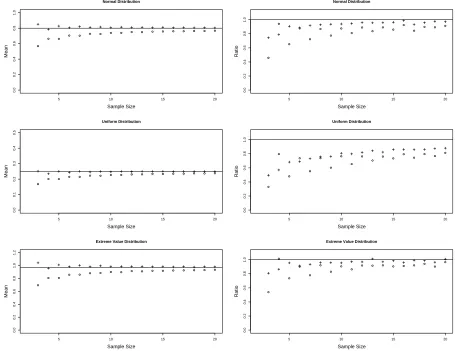
Figure 1.1: Left Side: Monte Carlo Estimates of Expectations of the Sample Means for each of the scale variables,Z andZ∗

versus Sample Size. Right Side: Monte Carlo Estimates (n_∗s2_µ_b)/s2 for Z and Z∗

versus Sample Size. _{◦ ◦ ◦} LevMed Scale or Z, +++ Modified LevMed Scale or Z∗

The left panels of Figure 1.1 give these average estimates µb versus sample size

(29)

value(0,1) distributions. The horizontal line is for the desired target θ2. Clearly the

“+” symbols for the modified LevMed variable are much more stable as n changes

than the LevMed variable represented by open circles. For example, the values

esti-mated by the mean of the LevMed variables at n = 3 and n = 6 are quite different,

whereas the corresponding values for the modified LevMed variables are quite close.

By n = 10 both sets of means are fairly stable, although the means of the

modi-fied variables, Z∗

are closer on average to the true values of θ2, 0.80, 0.25, and 0.97,

respectively, for the three distributions.

The average of the sample variances is s2 _{= (1}_/S₎PS

i=1s2i. We also obtain the Monte Carlo sample variance of the µib, s2

b

µ = (S−1)

−₁PS

i=1(bµi −µb)2. This latter quantity estimates var(µib), the true variance of the mean estimate. Validity of the

F test requires that var(µ_bi) be estimated by s2/n for each sample. Thus, we want s2 _≈ _n_∗_s2

b

µ. To examine whether this relationship holds, we calculated the ratio (n_∗s2

b

µ)/s2 for each of the two scale variables for each sample size and distribution. If this ratio is less than one, then the sample variances are too large on average, and

we might extrapolate that the denominator of the F statistic will be too large on

average.

The right panels of Figure 1.1 give these ratios for the three distributions. The

horizontal line is for the target value of 1. Again, we see that the modified LevMed

variables are more stable as n changes and also closer to the target value than the

(30)

distribution than for the other two distributions. The LevMed ratio is especially low

for n = 3. This can be anticipated due to the single 0 value inflating the sample

variance.

Correlation within the Samples

In the usual one-way ANOVA F test, one of the assumptions is that the

observa-tions within samples are independent. In this part, we focus on the correlation within

the samples for the scale variables Z and Z∗

.

In the simulation, the distributions are again normal, uniform, and extreme value.

The sample sizes configurations are: (I) n=3, (II) n=4, (III) n=5, (IV) n=6, (V)

n=20 and (VI) n=100. The number of Monte Carlo replications is S=10,000. The

within-sample correlation estimates are summarized in Table 1.1. We compute these

entries as follows. First, we generate a sample _{X1,_{· · ·} , Xn_}, then center them to

get the LevMed variables, _{Zj, j = 1,_{· · ·} , n_} , or the modified LevMed variables,

{Z∗

j, j = 1,· · · , n−1}. After that, we calculate the correlation between every pair of scale variables and get the average. For example, whenn = 3, we generate a random

sample, _{X1, X2, X3_}. After centering, we get the LevMed variables, _{Z1, Z2, Z3_}.

After that, we compute estimated correlations across all S samples between Z1 and

Z2, between Z1 and Z3 and between Z2 and Z3. The average of the 3 estimated

correlations is the entry for LevMed under n= 3.

(31)

medians instead of sample medians to calculate the Z values. As we expect, the

correlation estimates for the LevMed(θ1) are essentially 0 for all the cases. For small

sample sizes, both the LevMed variables and the modified LevMed variables lead to

negative within-sample correlations. The effect of negative correlation within samples

is that the sample variance divided by sample size overestimates the variance of the

corresponding mean, causing the test to be conservative. It is apparent that the

within-sample correlations are more strongly negative for the LevMed variables than

for the modified variables, for n odd and small.

Table 1.1: Estimates of Correlations within Samples for the Scale Variables Sample Size

Distribution Test n=3 n=4 n=5 n=6 n=20 n=100

Normal LevMed(θ1) 0.00 0.00 0.01 0.00 0.00 0.00

LevMed ₋0.21 ₋0.01 ₋0.07 ₋0.02 0.00 0.00 MLM ₋0.15 ₋0.07 ₋0.04 ₋0.02 0.00 0.00 Uniform LevMed(θ1) 0.00 0.00 0.00 0.00 0.00 0.00 LevMed ₋0.29 ₋0.05 ₋0.12 ₋0.04 ₋0.01 0.00 MLM ₋0.25 ₋0.16 ₋0.10 ₋0.06 ₋0.01 0.00 Extreme LevMed(θ1) 0.00 0.00 0.00 0.00 0.00 0.00 Value LevMed ₋0.18 0.00 ₋0.06 ₋0.02 0.00 0.00 MLM ₋0.12 ₋0.05 ₋0.03 ₋0.02 0.00 0.00 LevMed(θ1) is LevMed using known medians. Entries are based on 10,000 replications and have standard error _≤0.01.

Correlation between the Numerator and Denominator of the F Statistics

We also assess the correlation between SSR and SSE based on each of the two scale

variables because under the usual ANOVA assumptions, these two sums of squares

(32)

and SSE is the within-group or denominator sum of squares, for the F statistic.

For example, for the LevMed variables _{Zij, i = 1,_{· · ·} , k;j = 1,_{· · ·} , ni_}, SSR is

Pk

i=1ni(Zi·−Z··)2, and SSE is

Pk i=1

Pni

j=1(Zij −Zi·)2, where Z_i·=

Pni

j=1Zij/ni and Z·· =

Pk i=1

Pni

j=1Zij/N. Thus the F statistic (1.6) can be written as

F = SSR/df(SSR)

SSE/df(SSE). (1.15)

In the simulation, the distributions are again normal, uniform, and extreme value.

The sample size configurations are: (I) n=3, (II) n=4, (III) n=5, (IV) n=6, (V) n=20

and (VI) n=100. The group size configurations are: (i) k=2, (ii) k=4 and (iii) k=8.

The number of Monte Carlo replications is S=10,000. The correlation estimates

between SSR and SSE are summarized in Table 1.2. The entries labeled LevMed(θ1)

are results for the LevMed variable using true medians instead of sample medians.

The point is that skewness of the variables will cause some amount of correlation, but

the best we might hope for is the correlation present when we use known medians.

For all distributions at n = 3, the correlations for the modified LevMed variables

are closer to the correlations of the known median case than are the original LevMed

variables. This reverses at the normal and uniform for n= 4. Generally, the

correla-tions are a little closer for the modified variables, but we have trouble drawing strong

(33)

Table 1.2: Estimates of Correlation between SSR and SSE

Sample Size

Distribution k Test n=3 n=4 n=5 n=6 n=20 n=100

Normal 2 LevMed(θ1) 0.12 0.11 0.11 0.08 0.05 0.03

LevMed 0.38 0.10 0.26 0.07 0.06 0.03

MLM 0.23 0.17 0.18 0.10 0.06 0.03

4 LevMed(θ1) 0.15 0.14 0.12 0.13 0.08 0.03

LevMed 0.47 0.12 0.29 0.14 0.10 0.03

MLM 0.26 0.22 0.19 0.17 0.10 0.03

8 LevMed(θ1) 0.17 0.14 0.14 0.13 0.08 0.03

LevMed 0.48 0.10 0.29 0.14 0.09 0.03

MLM 0.27 0.21 0.18 0.17 0.08 0.03

Uniform 2 LevMed(θ1) ₋0.28 ₋0.25 ₋0.25 ₋0.23 ₋0.15 ₋0.06 LevMed 0.12 ₋0.21 0.03 ₋0.17 ₋0.07 ₋0.04 MLM 0.09 ₋0.15 0.00 ₋0.12 ₋0.07 ₋0.04 4 LevMed(θ1) ₋0.34 ₋0.32 ₋0.30 ₋0.27 ₋0.16 ₋0.09 LevMed 0.15 ₋0.27 0.03 ₋0.22 ₋0.09 ₋0.08 MLM 0.11 ₋0.19 ₋0.03 ₋0.16 ₋0.09 ₋0.08 8 LevMed(θ1) ₋0.38 ₋0.36 ₋0.33 ₋0.32 ₋0.19 ₋0.09 LevMed 0.18 ₋0.29 0.04 ₋0.23 ₋0.11 ₋0.09 MLM 0.13 ₋0.21 ₋0.02 ₋0.16 ₋0.10 ₋0.09 Extreme Value 2 LevMed(θ1) 0.58 0.51 0.49 0.44 0.29 0.12

LevMed 0.65 0.35 0.50 0.37 0.24 0.10

MLM 0.53 0.48 0.45 0.41 0.24 0.10

4 LevMed(θ1) 0.63 0.60 0.53 0.51 0.32 0.17

LevMed 0.74 0.47 0.54 0.43 0.28 0.14

MLM 0.64 0.59 0.48 0.48 0.28 0.14

8 LevMed(θ1) 0.64 0.60 0.55 0.55 0.35 0.17

LevMed 0.77 0.45 0.59 0.47 0.30 0.14

MLM 0.65 0.59 0.53 0.51 0.30 0.14

LevMed(θ1) is LevMed using true medians. Entries are based on 10,000 replications and have standard error from 0.007 to 0.026.

Discussion

The simulation results of the previous subsections suggest that an F statistic

(34)

the original LevMed variables. However, because there are a number of competing

aspects, we proceed to a direct comparison of the test procedures in the next section.

1.3 Simulations

1.3.1 Other Tests for equality of variances or Scale

Our goal in this section is to compare by simulation the modified LevMed

proce-dures including the MLM test and the MLM-BA test to the classical LevMed

pro-cedure and to some other tests for equality of variances or scale. Because it is well

known that normal-theory tests such as Bartlett’s test are sensitive to non-normality,

and these have been reported on extensively elsewhere, we will not consider nonrobust

normal-theory tests here. The other robust tests used in our simulation are defined

in the next few subsections.

Shoemaker’s Test

Shoemaker (2003) proposed a new homogeneity of variances test that is robust to

non-normality. Let s2

i be the sample variance of theith sample,{Xij, j = 1,· · · , ni}, and qi = ln(s2i). Shoemaker (2003, p. 107) suggests

χ2 = k

X

i=1

(qi−q)2 1

ni−₁

b

µ4

b

σ4 −

ni−3

ni

(35)

where µ4b = P_iP_j(Xij ₋ Xi)4_/N _and _b_σ2 ₌ P

i(ni − 1)s2i/N. The denominator of (1.16) is an estimate of var(qi) designed for small samples. Shoemaker (2003)

suggested using the harmonic mean of ni’s, nh = 1 k

n1+ 1

n2+

···₊1

nk

instead of individual

ni in the formula (1.16). The critical values of χ2 _{are obtained from a chi-squared}

distribution with k₋1 degrees of freedom.

Procedure Based on Gini’s Mean Difference

Miller (1968) proposed a general method of constructing spread variables to be

used in the ANOVA F statistic based on jackknife pseudo-values. Here we use the

Miller idea with a well-known scale estimator, Gini’s mean difference, which is highly

efficient across a range of distributions (e.g., see Johnson and Kotz, 1970, p. 67).

For two independent observations from the ith group, Gini’s mean difference scale

parameter is θi = E_|Xi1₋Xi2_|. It is unbiasedly estimated by the U-statistic

b

θi = 1 ni

2

X

j<k

|Xij −Xik|

or by the simpler to compute L-statistic version

b

θi = _n1_i 2

ni

X

j=1

(2j₋ni₋1)Xi(j),

(36)

To implement the Miller method, define the pseudo-values for the ith sample as

uij =niθib ₋(ni₋1)θi,b−j,

where the notation θi,b−j refers to the estimator in the ith group with Xij removed

from the sample. The Gini test is then based on the one-way ANOVA F statistic of

the new variables,

FGINI = P

ini(¯ui·−u¯··)2/(k−1)

P

i

P

j(uij −u¯i·)2/

P

i(ni−1)

(1.17)

where ¯ui =Puij/ni and ¯u·· =

P P

uij/N. The critical values of FGINI are obtained

from the F-distribution withk₋1 andN ₋k degrees of freedom.

Bootstrap Version of the LevMed Test

Boos and Brownie (1989) introduced the bootstrap technique for tests of scale

equality. Basically, the idea is to resample from the pooled set of residuals obtained

by subtracting group trimmed means within each sample. In the simulations of the

next subsection, we include a bootstrap version of LevMed. That is, the p-values

for the LevMed F statistic are obtained from a bootstrap resample procedure rather

than from the F distribution. Details may be found in Boos and Brownie (1989) or

(37)

1.3.2 Null Simulations

Comparison with Other Tests for Variances

We compare the Type I error robustness of the modified LevMed (MLM) test and

the MLM-BA test to the other four tests: the LevMed test (LM), Shoemaker’s (SH)

test, the F test on pseudo-values based on Gini’s mean difference (Gini), and the

bootstrap version of LevMed (BLM). The three distributions are: (1) Normal (0,1),

(2) Uniform (0,1), and (3) Extreme Value (0,1). The group size configurations are: (i)

k=2, (ii) k=4, and (iii) k=8. In the balanced design, the sample size configurations

are: (I) n = 3, (II) n = 4, (III) n = 5, (IV) n = 6, (V) n = 7, (VI) n = 8, (VII)

n = 9, (VIII) n = 10, (IX) n = 20, and (X) n = 100. We use S=1,000 Monte Carlo

replications. For BLM, the bootstrap replication size is B = 499. The nominal Type

I error rate is 0.05.

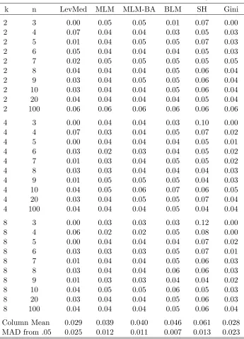
We summarize the results in Tables 1.3-1.5 for the three distributions, respectively.

Note that we only report two decimal places in the tables because the standard error

of the entries is approximately p(.95)(.05)/1000 =.007.

Tables 1.3-1.5 show that all six tests except Shoemaker’s test and LevMed for

n= 4 are conservative. Shoemaker’s test is liberal for many cases. At the bottom of

these three tables we have calculated a column mean and the mean absolute deviation

from .05, MAD = (1/30)P_|entry ₋.05_|. The column mean shows that the new

modified LevMed (MLM) is less conservative on average compared to the LevMed

(38)

Table 1.3: Estimated Levels for the Normal Distribution,α = 0.05

k n LevMed MLM MLM-BA BLM SH Gini

2 3 0.00 0.05 0.05 0.01 0.07 0.00

2 4 0.07 0.04 0.04 0.03 0.05 0.03

2 5 0.01 0.04 0.05 0.05 0.07 0.03

2 6 0.05 0.04 0.04 0.04 0.05 0.03

2 7 0.02 0.05 0.05 0.05 0.05 0.05

2 8 0.04 0.04 0.04 0.05 0.06 0.04

2 9 0.03 0.04 0.05 0.05 0.06 0.04

2 10 0.03 0.04 0.04 0.05 0.06 0.04

2 20 0.04 0.04 0.04 0.04 0.05 0.04

2 100 0.06 0.06 0.06 0.06 0.06 0.06

4 3 0.00 0.04 0.04 0.03 0.10 0.00

4 4 0.07 0.03 0.04 0.05 0.07 0.02

4 5 0.00 0.04 0.04 0.04 0.05 0.01

4 6 0.03 0.02 0.03 0.04 0.05 0.02

4 7 0.01 0.03 0.04 0.05 0.05 0.02

4 8 0.03 0.03 0.04 0.04 0.04 0.03

4 9 0.01 0.05 0.05 0.05 0.04 0.03

4 10 0.04 0.05 0.06 0.07 0.06 0.05

4 20 0.03 0.04 0.05 0.05 0.07 0.04

4 100 0.04 0.04 0.04 0.05 0.04 0.04

8 3 0.00 0.03 0.03 0.03 0.12 0.00

8 4 0.06 0.02 0.02 0.05 0.08 0.00

8 5 0.00 0.04 0.04 0.04 0.07 0.02

8 6 0.03 0.03 0.03 0.05 0.07 0.01

8 7 0.01 0.04 0.04 0.05 0.06 0.03

8 8 0.03 0.04 0.04 0.06 0.06 0.03

8 9 0.01 0.03 0.03 0.04 0.04 0.02

8 10 0.04 0.05 0.05 0.06 0.05 0.03

8 20 0.03 0.04 0.04 0.05 0.06 0.03

8 100 0.04 0.04 0.04 0.05 0.06 0.04

Column Mean 0.029 0.039 0.040 0.046 0.061 0.028

MAD from .05 0.025 0.012 0.011 0.007 0.013 0.023

Note: Entries based on 1,000 replications. Standard error of main

entries_≤(.88_∗.12/1000)1/2 ₌_.₀₁_._{“MAD from .05” is the mean}

(39)

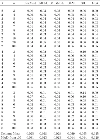
Table 1.4: Estimated Levels for the Uniform distribution, α= 0.05

2 3 0.00 0.03 0.03 0.02 0.06 0.00

2 4 0.09 0.05 0.06 0.05 0.05 0.04

2 5 0.01 0.04 0.04 0.04 0.04 0.03

2 6 0.04 0.04 0.03 0.04 0.04 0.03

2 7 0.01 0.04 0.04 0.05 0.04 0.03

2 8 0.04 0.04 0.04 0.05 0.04 0.04

2 9 0.02 0.03 0.03 0.04 0.04 0.04

2 10 0.04 0.04 0.04 0.05 0.04 0.04

2 20 0.04 0.05 0.05 0.06 0.06 0.06

2 100 0.04 0.04 0.04 0.05 0.05 0.05

4 3 0.00 0.02 0.02 0.01 0.10 0.00

4 4 0.09 0.02 0.02 0.06 0.06 0.01

4 5 0.00 0.01 0.01 0.02 0.05 0.01

4 6 0.03 0.02 0.02 0.03 0.05 0.02

4 7 0.00 0.03 0.03 0.04 0.05 0.03

4 8 0.03 0.03 0.03 0.04 0.04 0.03

4 9 0.01 0.03 0.03 0.04 0.04 0.03

4 10 0.02 0.02 0.02 0.04 0.04 0.02

4 20 0.03 0.03 0.03 0.04 0.04 0.03

4 100 0.05 0.06 0.06 0.07 0.06 0.05

8 3 0.00 0.01 0.01 0.01 0.14 0.00

8 4 0.07 0.01 0.02 0.06 0.10 0.01

8 5 0.00 0.01 0.01 0.01 0.08 0.01

8 6 0.02 0.01 0.01 0.03 0.06 0.01

8 7 0.00 0.02 0.02 0.03 0.06 0.02

8 8 0.02 0.01 0.01 0.04 0.04 0.01

8 9 0.00 0.01 0.01 0.02 0.04 0.01

8 10 0.01 0.02 0.02 0.04 0.04 0.02

8 20 0.02 0.03 0.03 0.04 0.06 0.03

8 100 0.03 0.04 0.04 0.05 0.04 0.04

Column Mean 0.025 0.028 0.028 0.039 0.055 0.025

MAD from .05 0.031 0.023 0.023 0.014 0.014 0.026

entries_≤(.86_∗.14/1000)1/2 =.01.“MAD from .05” is the mean

(40)

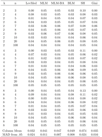
Table 1.5: Estimated Levels for the Extreme Value distribution, α= 0.05

2 3 0.00 0.05 0.05 0.03 0.10 0.00

2 4 0.08 0.03 0.05 0.03 0.08 0.03

2 5 0.01 0.04 0.05 0.04 0.07 0.03

2 6 0.04 0.03 0.05 0.05 0.07 0.04

2 7 0.03 0.06 0.06 0.07 0.08 0.06

2 8 0.04 0.05 0.06 0.05 0.07 0.05

2 9 0.03 0.06 0.07 0.06 0.08 0.05

2 10 0.03 0.03 0.04 0.04 0.06 0.04

2 20 0.04 0.05 0.06 0.05 0.08 0.05

2 100 0.04 0.04 0.04 0.04 0.05 0.04

4 3 0.00 0.03 0.05 0.03 0.11 0.00

4 4 0.07 0.03 0.04 0.05 0.06 0.02

4 5 0.01 0.02 0.03 0.03 0.07 0.02

4 6 0.03 0.03 0.04 0.05 0.08 0.04

4 7 0.01 0.03 0.04 0.04 0.06 0.03

4 8 0.04 0.05 0.06 0.06 0.09 0.05

4 9 0.03 0.05 0.06 0.06 0.06 0.05

4 10 0.04 0.05 0.06 0.06 0.08 0.05

4 20 0.04 0.04 0.04 0.05 0.06 0.05

4 100 0.05 0.05 0.05 0.05 0.05 0.05

8 3 0.00 0.04 0.05 0.04 0.13 0.00

8 4 0.09 0.04 0.04 0.08 0.11 0.02

8 5 0.00 0.03 0.04 0.04 0.08 0.02

8 6 0.04 0.04 0.04 0.06 0.08 0.02

8 7 0.01 0.04 0.05 0.05 0.07 0.04

8 8 0.03 0.03 0.04 0.05 0.06 0.03

8 9 0.01 0.03 0.04 0.05 0.05 0.03

8 10 0.04 0.05 0.05 0.06 0.06 0.04

8 20 0.03 0.05 0.05 0.05 0.06 0.04

8 100 0.04 0.05 0.05 0.05 0.05 0.05

Column Mean 0.032 0.041 0.047 0.049 0.074 0.035

MAD from .05 0.024 0.011 0.007 0.008 0.024 0.016

entries_≤(.87_∗.13/1000)1/2 =.01.“MAD from .05” is the mean

(41)

mean difference is the most conservative overall but appears to be slightly better than

the LevMed test for the extreme value distribution. An important conclusion from

these tables is that the new modified LevMed (MLM) is a definite improvement over

the established LevMed procedure for sample sizes n = 3 to n = 5. That was our

original goal for creating the modified procedure. Results from the MLM-BA test are

similar to the results from the MLM test for the normal distribution and the uniform

distribution. Under the extreme value distribution, the MLM-BA test improves the

performance of the MLM test, which shows that the Box-Andersen correction plays

an important role for skewed distributions. The good point is that the MLM-BA test

performs as well as the bootstrapped version, BLM.

Table 1.6 summarizes some results for unbalanced designs. The results for the

unbalanced designs are consistent with those for the balanced design. The modified

LevMed test also improves the null performance under the unbalanced design,

espe-cially for the normal and extreme value distributions. At the bottom of the table

we have also calculated a column mean and the MAD from .05. The column mean

shows that the modified LevMed test is less conservative on average compared to the

LevMed test, especially for the normal and extreme value distributions. The MAD

from .05 shows that the modified LevMed test can lead to estimates of significance

levels closer to the nominal rate than the LevMed test. Table 1.6 does not include

(42)

Table 1.6: Estimated Levels of Nominal 0.05 tests for Unbalanced Designs Distribution

Sample Size Normal Uniform Extreme Value

LevMed MLM LevMed MLM LevMed MLM

(5,15) 0.02 0.05 0.02 0.04 0.02 0.04

(3,4) 0.04 0.05 0.04 0.04 0.04 0.04

(3,8) 0.01 0.04 0.04 0.02 0.02 0.05

(4,7) 0.03 0.03 0.03 0.03 0.04 0.04

(5,20) 0.03 0.04 0.07 0.05 0.02 0.06

(6,19) 0.04 0.04 0.04 0.03 0.03 0.04

(5,5,15,15) 0.01 0.04 0.02 0.02 0.03 0.06

(5,5,5,15) 0.00 0.04 0.01 0.03 0.01 0.05

(5,15,15,15) 0.02 0.05 0.02 0.03 0.03 0.05

(3,3,4,4) 0.03 0.02 0.03 0.03 0.03 0.05

(3,3,3,4) 0.01 0.04 0.01 0.01 0.01 0.04

(3,4,4,4) 0.05 0.03 0.05 0.02 0.05 0.04

(4,4,7,7) 0.03 0.04 0.02 0.02 0.04 0.04

(4,4,4,7) 0.04 0.03 0.04 0.03 0.04 0.03

(4,7,7,7) 0.01 0.03 0.01 0.03 0.02 0.03

(3,3,8,8) 0.02 0.04 0.02 0.01 0.01 0.05

(3,3,3,8) 0.01 0.05 0.01 0.02 0.01 0.05

(3,8,8,8) 0.03 0.04 0.03 0.02 0.03 0.06

(5,5,5,5,15,15,15,15) 0.01 0.04 0.01 0.01 0.02 0.06

(5,5,5,5,5,5,5,15) 0.00 0.03 0.00 0.01 0.01 0.06

(5,15,15,15,15,15,15,15) 0.02 0.04 0.00 0.02 0.02 0.04

Column Mean 0.021 0.037 0.024 0.025 0.025 0.047

MAD from 0.05 0.029 0.013 0.027 0.025 0.025 0.009

Entries are based on 1,000 replications. Standard Error of individual entries

≤(.93_∗.07/1000)1/2 _{= 0}_.₀₁

Relationship between the Estimated Type I Error Rates and Sample Sizes

and Number of Groups

To further illustrate the comparison between the LevMed test and the new

modi-fication, we have increased the Monte Carlo sample size to S=10,000 replications and

(43)

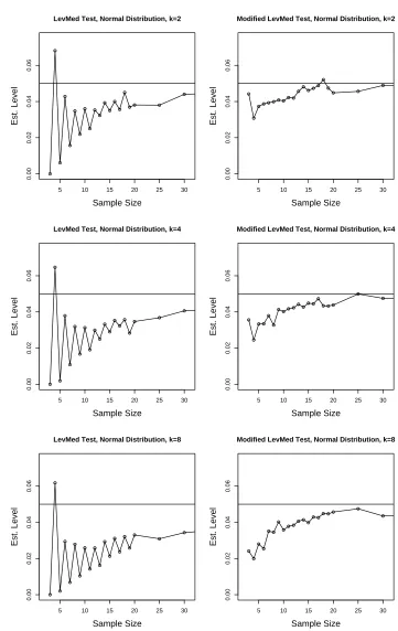
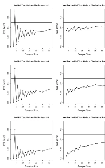
with the LevMed on the left and the new modification on the right. Figures 1.2-1.4

are for the normal distribution, the uniform distribution, and the extreme value

dis-tribution, respectively. Figures 1.2-1.4 are at the end of the chapter due to space

considerations.

The plots for the modified LevMed test are much more stable than those for the

LevMed test. The ranges of the estimated levels (from 0.02 to 0.05) for the modified

LevMed test are much smaller than the ranges of the LevMed test (from 0 to 0.07) for

small sample sizes. As k increases, both the LevMed test and the modified LevMed

test become more conservative for small sample sizes.

Finally, we give two more pages of plots at the end of the chapter to illustrate

better how the Type I error rates of the modified LevMed procedure change as k

increases. In Figure 1.5 we have taken the data from Figures 1.2-1.4 and put the

graphs for a given distribution on the same row with k increasing as we move from

left to right. In addition we have used a local smoother to track the trend as sample

size increases. In Figure 1.6 we have put the local smoothers for all three group

numbers, k = 2, k = 4, and k = 8, on the same plot but without the individual

points. In both sets of plots we can see that an increase ink causes the procedure to

(44)

1.3.3 Power

We now compare the power of the modified LevMed test (MLM) and the

MLM-BA test to power of the other 4 tests. The sample size configurations are n=3, 4, 5, 6,

7, 8, 9, 10, and 20. The variance configurations are (1:4), (1:8), (1:6:11:16), (1:1:1:16),

(1:1:1:8:8:8:16:16) and (1:1:1:1:1:1:16:16). We use S=1,000 Monte Carlo replications

with the nominal rate equal to 0.05. The results are summarized in Tables 1.11-1.13

at the end of the chapter.

In these tables we see important power gains at n= 3,5,7,and 9 for the modified

LevMed procedure compared to LevMed. When sample sizes reach n = 20 all the

procedures are similar in power. A very crude summary is to take the mean of the

columns for each table. The results are summarized in Table 1.7. The underline

emphasizes the most powerful test for every distribution. Thus, the modified

pro-cedure has an overall gain in power of about .05 when compared to LevMed, and

the bootstrapped LevMed has an average .02 gain in power compared to the

mod-ified procedure. Amazingly, the MLM-BA test generally has higher power than the

bootstrapped LevMed test and the MLM-BA test is much simpler to perform, which

indicates that the Box-Andersen correction can improve the power of the modified

LevMed test. The Gini procedure has power in between the LevMed and the modified

LevMed procedure. The Shoemaker procedure has good power, but the comparison

(45)

Table 1.7: Comparison of Average Power Among the Six Tests Distribution

Test Normal Uniform Extreme Value

LevMed 0.48 0.53 0.43

MLM 0.53 0.57 0.48

MLM-BA 0.56 0.60 0.52

BLM 0.55 0.59 0.50

SH 0.54 0.61 0.51

Gini 0.51 0.59 0.45

Note: Entries based on the results of Table 1.11-1.13.

Standard error of entries_≤0.002.

1.4 Example

Phadke et. al (1983) reported on an off-line quality control experiment in the

fabrication of integrated circuit chips. We will use part of the data to illustrate the 6

tests used in the simulations.

In order to choose process conditions to minimize variance in contact window

sizes of integrated circuit chips, Phadke et. al (1983) conducted an experiment with

18 combinations of levels of factors. For every experimental unit (of 18

experimen-tal units), there are 5 specific measured locations such as “Top,” “Bottom,” “Left,”

“Right,” and “Center” locations. Most of the experimental units have 10

observa-tions (2 measurements for every location) except units 5, 15 and 18 which have 5

observations (only 1 measurement for every location). We use part of the “pre-etch”

window size data to compare the six tests. In our example, if we use the

experimen-tal units 1-4, then k = 4 and if we use experiments 1-8, then k = 8. If we use the

(46)

unit is measured at the “Top,” “Center,” “Bottom,” locations. If we use the first

4 observations for every experimental unit, then n = 4, and the experimental unit

is measured at the “Top,” “Center,” “Bottom,” and “Left” locations. When n = 5,

the experimental unit is measured at the “Top,” “Center,” “Bottom,” “Left,” and

“Right” locations.

Table 1.8 summarizes the data including the mean and the sample standard

devi-ation for every case. The standard devidevi-ation is a measure of varidevi-ation within a chip

and not between chips produced under the same factor settings.

Table 1.8: Summary Statistics of Data from Off-Line Quality Control Study

Statistic Mean SD

Size n=3 n=4 n=5 n=3 n=4 n=5

h=1 2.53 2.53 2.52 0.10 0.08 0.07 h=2 2.72 2.69 2.66 0.05 0.07 0.10 h=3 2.77 2.72 2.64 0.06 0.12 0.19 h=4 2.10 2.07 2.08 0.10 0.10 0.09 h=5 1.91 1.88 1.87 0.15 0.13 0.12 h=6 2.54 2.52 2.52 0.03 0.05 0.04 h=7 2.03 2.02 2.02 0.07 0.06 0.05 h=8 3.42 3.34 3.28 0.26 0.27 0.26 h=9 2.99 2.91 2.88 0.08 0.18 0.17 h=10 2.57 2.54 2.51 0.11 0.10 0.11 h=11 3.24 3.23 3.21 0.07 0.06 0.06 h=12 3.29 3.28 3.24 0.07 0.06 0.09 h=13 2.59 2.58 2.58 0.03 0.03 0.03 h=14 2.28 2.26 2.27 0.15 0.13 0.11 h=15 2.49 2.47 2.46 0.03 0.04 0.04 h=16 2.64 2.66 2.64 0.10 0.09 0.08

From Table 1.9, we can see that the MLM test, the MLM-BA test and the BLM

(47)

Table 1.9: P-Values for tests of equality of within chip variance using subsets of data from an Off-Line Quality Control Study

k=4 k=8 k=16

Test n=3 n=4 n=5 n=3 n=4 n=5 n=3 n=4 n=5

LevMed 0.83 0.87 0.32 0.37 0.03 0.18 0.73 0.07 0.13 MLM 0.63 0.90 0.18 0.04 0.12 0.09 0.29 0.24 0.03 MLM-BA 0.63 0.90 0.13 0.04 0.10 0.07 0.29 0.23 0.03 BLM 0.59 0.86 0.12 0.04 0.05 0.06 0.11 0.09 0.01 SH 0.67 0.84 0.41 0.51 0.54 0.17 0.80 0.61 0.18 Gini 0.83 0.92 0.28 0.37 0.19 0.10 0.73 0.39 0.06

sample sizes because they can’t detect difference in variances for the case with k = 8

and n = 3 or the case with k = 8 and n = 4. The LevMed test does not detect

heterogeneity of variances for the case with k = 8 and n = 3, while the MLM test

and the BLM test provide evidence of variance heterogeneity. On the other hand, the

MLM test misses the heterogeneity of variances for the case with k = 8 and n = 4,

while the LevMed test and the BLM test can detect it. This is in part because the

LevMed test tends to be liberal and consequently has more power than the MLM test

for small and even sample sizes. In contrast, the MLM test has more power than the

LevMed test for the small and odd sample sizes because it avoids the conservative

(48)

1.5 Comparison with the Hines LevMed Test (Hines

and Hines, 2000)

Hines and Hines (2000) proposed a modification of the LevMed test (the Hines

LevMed test) by removing linear dependencies (structural zeros) among the LevMed

variables, which is similar to our Modified LevMed test. Suppose that (Zi(1),_{· · ·} , Zi(ni))

are the ordered LevMed variables for the ith group. If the sample size ni is odd,

the Hines LevMed test deletes the smallest value, Zi(1) = 0. If the sample size is even, then Zi(1) = Zi(2) and the pair of values Zi(1) and Zi(2) is replaced by the pair

(Zi(2)₋Zi(1))/√2 ( = 0) and (Zi(2)+Zi(1))/√2. The resulting structural zero is then

deleted. ANOVA is then applied to the remaining Z values. When the sample size

is odd for all k groups, the Hines test is the same as the MLM test. When any of

the sample sizes is even, the smallest Z value for that group is (Zi(1)+Zi(2))/√2 for

Hines LevMed, compared to (Zi(1)+Zi(2))/2 for the MLM procedure.

To further illustrate the comparison between the modified LevMed and the Hines

test, we have made a series of plots of the estimated Type I error versus sample sizes

per group with the Hines test on the left and the MLM on the right. Figures

1.7-1.9 are for the normal distribution, the uniform distribution, and the extreme value

distribution, respectively. These three figures are at the end of the chapter due to

space considerations. For n odd, the Hines and MLM tests are the same, but for n

(49)

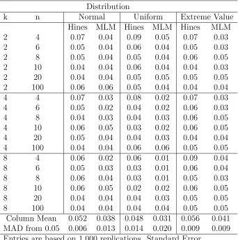
Table 1.10: Comparison of Estimates of Levels between the Modified LevMed test and Hines test for Even Sample Sizes

Distribution

k n Normal Uniform Extreme Value

Hines MLM Hines MLM Hines MLM

2 4 0.07 0.04 0.09 0.05 0.07 0.03

2 6 0.05 0.04 0.06 0.04 0.05 0.03

2 8 0.05 0.04 0.05 0.04 0.06 0.05

2 10 0.04 0.04 0.06 0.04 0.04 0.03

2 20 0.04 0.04 0.05 0.05 0.05 0.05

2 100 0.06 0.06 0.05 0.04 0.04 0.04

4 4 0.07 0.03 0.08 0.02 0.07 0.03

4 6 0.05 0.02 0.04 0.02 0.06 0.03

4 8 0.04 0.03 0.04 0.03 0.06 0.05

4 10 0.06 0.05 0.03 0.02 0.06 0.05

4 20 0.05 0.04 0.04 0.03 0.04 0.04

4 100 0.04 0.04 0.06 0.06 0.05 0.05

8 4 0.06 0.02 0.06 0.01 0.09 0.04

8 6 0.05 0.03 0.03 0.01 0.06 0.04

8 8 0.06 0.04 0.03 0.01 0.05 0.03

8 10 0.06 0.05 0.02 0.02 0.06 0.05

8 20 0.04 0.04 0.04 0.03 0.05 0.05

8 100 0.04 0.04 0.04 0.04 0.05 0.05

Column Mean 0.052 0.038 0.048 0.031 0.056 0.041 MAD from 0.05 0.006 0.013 0.014 0.020 0.009 0.009 Entries are based on 1,000 replications. Standard Error

of individual entries _≤(.91_∗.09/1000)1/2 _{= 0}_.₀₁

n, levels of MLM are consistently conservative, whereas levels of the Hines test show

an oscillating pattern with peaks when n is even. Although similar to the odd/even

pattern for levels of LevMed (Figures 1.2 - 1.4), the Hines modification is clearly an

improvement over LevMed.

The plots for the modified LevMed test are more stable than those for the Hines

(50)

test are much smaller than the ranges of the Hines Levene test (from 0.02 to 0.09)

for the small sample sizes.

Because the Hines test is the same with the MLM test for odd sample sizes, Table

1.10 presents levels for the MLM and Hines tests only for even sample sizes. When

n = 4, the Hines test is liberal under all the three distributions. Under the normal

distribution and the uniform distribution, as k, the number of groups, increases, the

Hines test holds its levels better than MLM which becomes more conservative. Under

the extreme value distribution, the Hines test tends to be liberal while the MLM test is

conservative. Except at the extreme value distribution, based on the MAD summary,

the Hines test appears to hold its level better than the MLM test for n small and

even.

We also compare the Hines test to the other tests in terms of power by simulation.

Using the same seeds, Monte Carlo samples were generated for the 30 non-null cases

summarized in Table 1.7 for the six other tests. Power was obtained for each case

for the Hines test and average power was calculated. The resulting average powers

under the normal distribution, the uniform and the extreme value for the Hines test

are 0.55, 0.59 and 0.49, respectively. Compared to the MLM test, the Hines has

slightly greater power for the normal distribution and the uniform distribution due

to its liberal performance for n even and small. However, it does not perform as well

(51)

1.6 Conclusion

This chapter demonstrates that the modified LevMed (MLM) test can yield valid

levels and good power for most configurations studied. The MLM test performs

well for small and odd sample sizes, where the shortcomings of the LevMed test are

most pronounced. MLM, which differs from the Hines test only if some ni are even,

performs better than the Hines test under skewed distributions, in this case. Although

the modified LevMed test is inferior to the BLM test in terms of level and power, it

is much simpler than the BLM test. The Box-Andersen correction can improve the

power of the Modified LevMed test, especially for skewed distributions. In general

(52)

(53)

5 10 15 20 25 30 0.00 0.02 0.04 0.06 Sample Size Est. Level

LevMed Test, Normal Distribution, k=2

5 10 15 20 25 30

0.00 0.02 0.04 0.06 Sample Size Est. Level

Modified LevMed Test, Normal Distribution, k=2

5 10 15 20 25 30

Figure 1.2: Estimated levels versus sample sizes for the normal distribution. Standard deviations of plotted values are bounded by (40000)−1/2

(54)

LevMed Test, Uniform Distribution, k=2

5 10 15 20 25 30

Modified LevMed Test, Uniform Distribution, k=2

5 10 15 20 25 30

Figure 1.3: Estimated levels versus sample sizes for the uniform distribution. Stan-dard deviations of plotted values are bounded by (40000)−1/2

(55)

LevMed Test, Extreme Value Distribution, k=2

5 10 15 20 25 30

Modified LevMed Test, Extreme Value Distribution, k=2

5 10 15 20 25 30

Figure 1.4: Estimated levels versus sample sizes for the extreme value distribution. Standard deviations of plotted values are bounded by (40000)−1/2

(56)

5 10 15 20 25 30 0.00 0.01 0.02 0.03 0.04 0.05 0.06 Sample Size Est. Level k=2

5 10 15 20 25 30

0.00 0.01 0.02 0.03 0.04 0.05 0.06 Sample Size Est. Level k=4 Normal Distribution

5 10 15 20 25 30

0.00 0.01 0.02 0.03 0.04 0.05 0.06 Sample Size

Est. Level _k=8

5 10 15 20 25 30

0.00 0.01 0.02 0.03 0.04 0.05 0.06 Sample Size Est. Level k=2

5 10 15 20 25 30

0.00 0.01 0.02 0.03 0.04 0.05 0.06 Sample Size Est. Level k=4 Uniform Distribution

5 10 15 20 25 30

New Methods using Levene Type Tests for Hypotheses about Dispersion Differences

Biography

Acknowledgements

Contents

List of Figures

List of Tables

Chapter 1

The Modified LevMed Test for a

One-Way Design

1.1

Introduction

1.1.1

Normal Theory Tests

1.1.2

Robust Variance Tests

1.2

The LevMed Test and the Modified LevMed

Test

1.2.1

Model

1.2.2

The LevMed Test

1.2.3

The Modified LevMed Test

1.2.4

Small Sample Properties of the LevMed and Modified

LevMed Variables

1.3

Simulations

1.3.1

Other Tests for equality of variances or Scale

1.3.2

Null Simulations

1.3.3

Power

1.4

Example

1.5

Comparison with the Hines LevMed Test (Hines

and Hines, 2000)

1.6

Conclusion