Multicycle Adaptive Simulation of Boiling Water Reactor Core Simulators

Abstract

BRIGGS, CHRISTOPHER MICHAEL. Multicycle Adaptive Simulation of Boiling Water Reactor Core Simulators. (Under the direction of Paul J. Turinsky).

Adaptive simulation (AS) is an algorithm utilizing a regularized least squares

methodol-ogy to correct for the discrepancy between core simulators predictions and actual plant

mea-surements [1]. This is an inverse problem that will adjust the cross sections input to a core

simulator within their range of uncertainty to obtain better agreement with the plant

measure-ments. The cross section adjustments are constrained to their range of uncertainty using the

covariance matrix of the few-group cross sections and in imposing the regularization on the

least squares solution. This few-group covariance matrix is obtained using the covariance

matrix of the multi-group cross sections and the corresponding lattice physics sensitivity

matrix. To perform the adaption, one must also have the sensitivity matrix of the core

simula-tor. Constructing the sensitivity matrix of both the lattice physics code and core simulator

would be a daunting task using the traditional brute-force method of computing a forward

solve for a perturbation of every input. To avoid this, a singular value decomposition (SVD) is

used to construct a low rank approximation of the covariance matrices, thus drastically

reduc-ing the number of required forward solves.

Until now, AS has been used on a single depletion cycle to correct for discrepancies

result-ing from errors introduced by incorrect cross sections only. Adaptresult-ing to a sresult-ingle depletion

cycle means that the cross sections of cycle m were adjusted so that the core simulator better

predicts the actual measurements of cycle m (and future cycles if the algorithm is robust).

This, however, does not account for the reloaded burnt fuel number density errors at the

previous cycle. If adaption changes the cross sections of that burnt assembly in cycle m, those

cross sections should have also been changed in any cycle preceding m which would have

resulted in different BOC m number densities. This means that the number densities obtained

using the original cross sections are not consistent with the newly adapted cross sections.

Hence, the number densities input to a core simulator are not the actual values in the

reac-tor’s fuel assemblies for the burnt fuel. This discrepancy in isotopics is another component to

the discrepancy between the core simulator and actual observables. This means that the

adap-tion algorithm is adjusting cross secadap-tions to account for number density errors.

It is the goal of this research to 1) remove these inconsistencies between the adapted cross

sections and the burnt fuel BOC n number densities, and 2) ensure that adjusting cross

sec-tions to make up for number density errors does not corrupt the adaption. To do this, we

assume that to best predict cycle n (by correcting both cross sections and BOC number

densi-ties of cycle n), one must adapt cycles m through n-1 simultaneously, where cycle m is the

cycle in which the oldest assembly in cycle n is a fresh assembly. After adaption, the cross

sections must be used to deplete from cycle m to n. This will remove the number density

errors in two ways: 1) burnup healing, and 2) beginning the depletion of fresh assemblies in

cycles m through n-1 with the correct cross sections. To ensure the cross sections adjustments

are not overcompensating for the number density errors, we restrain their adjustment to stay

Multicycle Adaptive Simulation

of Boiling Water Reactor

Core Simulators

by

Christopher Michael Briggs

A thesis submitted to the Graduate Faculty of North Carolina State University

in partial fulfillment of the requirements of the Degree of

Master of Science

Nuclear Engineering

Raleigh, North Carolina 2007

APPROVED BY:

~,)(l/~--Semyon V. Tsynkov

Co-chair of Advisory Committee

ii

Dedication

iii

Biography

Christopher M. Briggs was born in Houston, TX on February 2nd, 1983. He received his

primary education locally in Houston, graduating from Scarborough High School in 2001. He

attended Texas A&M and received his Bachelor of Science in May 2005 from the Department

of Nuclear Engineering, graduating Magna Cum Laude. After A&M, Chris began his work

towards a Master’s of Science in Nuclear Engineering at North Carolina State University

under the direction of Dr. Paul J. Turinsky. He has accepted a position at Westinghouse

iv

Acknowledgements

There isn’t enough room on this page to properly thank those that made it possible for me

to complete my master’s work here at N.C. State. I would like to thank my family for the

bot-tomless well of support that kept me going through the hardest and most stressful of times

starting from day one. Their continuous self-sacrifice gave me all the time and resources I

could have ever needed to be where I am today. I would also like to thank Dr. Turinsky for

accepting me as a master’s student and teaching more than I ever imagined I could learn in

only two years. Next I would like to thank Dr. Paul Keller for his uncanny ability to fix

FOR-MOSA B when I broke it, without which I would have never been able to get my research off

the ground. At the opposite end of my research, I also want to thank both Dr. Abdel-Khalik

and Mr. Matthew Jessee for the long hours they both contributed to ensure my final product

withstood the most intense scrutiny. It is also worth noting the unwavering patience of Dr.

Turinsky and Dr. Abdel-Khalik for withstanding the endless stream of mindless mistakes I put

them through.

I would also like to thank my peers for their insight, support, and most importantly their

constant source of comical relief. This includes Kenny Anderson, Doug DeJulio, Jason Harp,

Ross Hays, Tyler Hickle, Matt Jessee, Tracy Stover, and Tim Wright. Lastly, even though

v

Table of Contents

List of Figures. . . vii

1. Introduction . . . 1

1.1 Scope of Work . . . 3

1.2 Core Simulators Overview. . . 4

1.2.1 Core Simulator Basics . . . 4

1.2.2 Various Core Simulators . . . 5

1.2.3 Core Simulator Input . . . 6

1.2.4 Simulation Errors . . . 7

1.2.5 Simulator Output . . . 9

1.3 Adaptive Simulation . . . 9

1.3.1 Necessary Traits . . . 10

1.3.2 Adaption Benefits . . . 12

1.3.3 Previous Adaption Methods . . . 12

2. Adaptive Simulation . . . 14

2.1 Least Squares Development. . . 14

2.1.1 Regularization Parameter. . . 16

2.2 Least Squares Continued . . . 19

2.3 Completing the Adaption. . . 20

3. Design and Virtual Cores . . . 25

3.1 Cross Section Perturbations . . . 26

3.2 Number Density Perturbation . . . 30

3.2.1 Core Simulator Software and Design Core . . . 31

3.2.2 Introducing the Number Density Errors . . . 32

4. Results . . . 34

4.1 Pre-Adaption Number Density Behavior. . . 34

4.1.1 Linear Response. . . 34

4.1.2 Burnup Healing and Fresh Fuel Loading. . . 35

4.2 Adaption Inputs . . . 37

4.2.1 Regularization Parameter. . . 37

vi

4.2.3 Cycle Weights . . . 39

4.3 Number Density Decrease vs. Adaption Inputs. . . 40

4.3.1 Constant Cycle Weight . . . 42

4.3.2 Constant keff Weight . . . 47

4.3.3 Constant Alpha . . . 48

4.3.4 Linearization Error. . . 49

4.4 Summary . . . 50

5. Conclusions. . . 65

6. Future Work. . . 67

vii

List of Figures

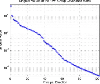
Figure 3.1: Singular values vs. principal direction. . . 28

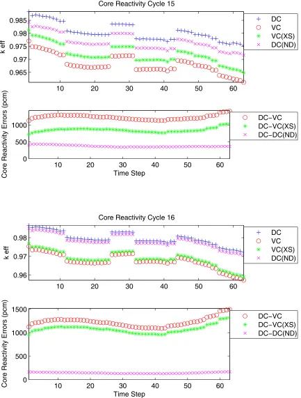
Figure 4.1: k_eff and pcm errors of cycles 15 and 16 resulting from cross section and number density errors . . . 52

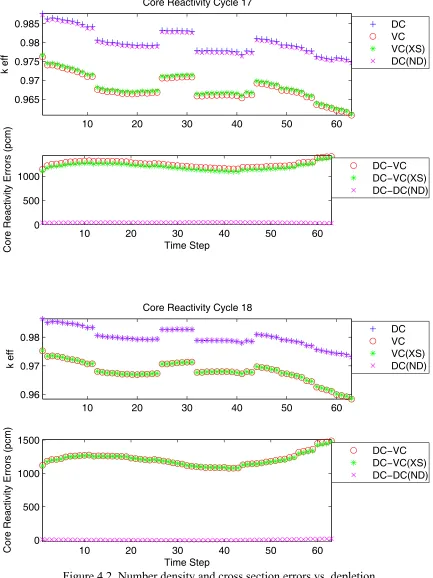
Figure 4.2: k_eff and pcm errors of cycles 17 and 18 resulting from cross section and number density errors . . . 53

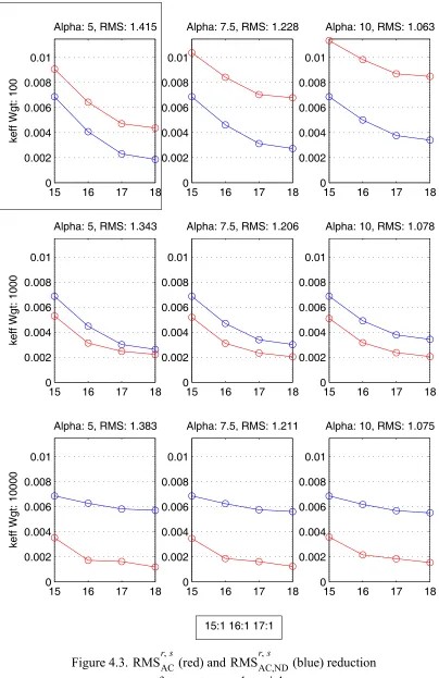
Figure 4.3: (red) and (blue) reduction for constant cycle weight . . . . 54

Figure 4.4: k_eff (blue) and nodal power (red) misfit for constant cycle weight . . . 55

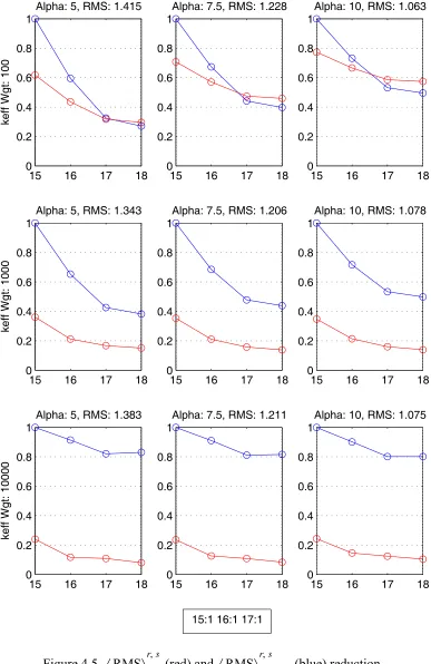
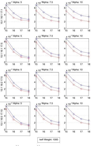
Figure 4.5: (red) and (blue) reduction for constant cycle weight 56 Figure 4.6: (red) and (blue) reduction for constant k_eff weight . . . 57

Figure 4.7: k_eff (blue) and nodal power (red) misfit for constant k_eff weight . . . 58

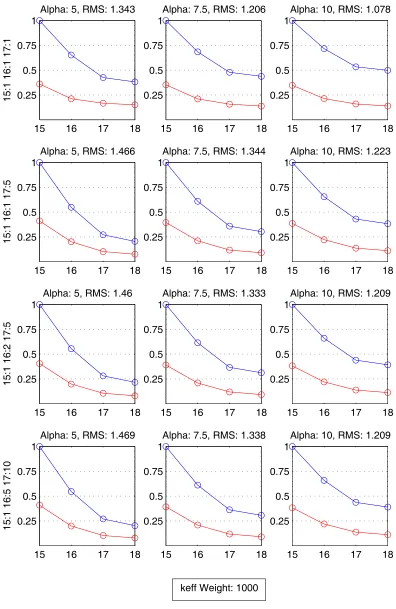
Figure 4.8: (red) and (blue) reduction for constant k_eff weight. . 59

Figure 4.9: (red) and (blue) reduction for constant alpha. . . 60

Figure 4.10: k_eff (blue) and nodal power (red) misfit for constant alpha . . . 61

Figure 4.11: Number density reduction for constant alpha . . . 62

Figure 4.12: Cycle 18 k_eff and pcm error for each core . . . 63

Figure 4.13: Nodal power RMS error: (blue), (green), and (black) . . . 64

RMSr s_AC, RMSr s_AC,ND,

RMS

〈 〉r s_AC, 〈RMS〉r s_AC,ND,

RMSr s_AC, RMSr s_AC,ND,

RMS

〈 〉r s_AC, 〈RMS〉r s_AC,ND,

RMSr s_AC, RMSr s_AC,ND,

RMSr

DC NP, RMS

r

AC NP,

RMSr

CHAPTER 1: INTRODUCTION 1

Chapter 1: Introduction

In the present day nuclear power industry, a reliable reactor core simulator for light water

reactor (LWR) cores is a crucial part of reactor design, economics, and safety. The

development of such a crucial tool is no trivial task, requiring design, construction, and testing

that can take years. These steps can require an exorbitant amount of time and money before

any worthwhile results are produced that justify the effort dedicated. Furthermore, even when

the core simulator is complete, it will inevitably have its own limitations that prevent it from

completely reproducing actual real plant data. To avoid this scenario, and for multiple reasons

to be discussed later, there has been an effort to improve the input data to existing core

simulators so that the simulator’s prediction of a reactor’s behavior are closer to that of the

real world reactor. Throughout this paper, this effort is known as adaptive simulation.

Adaptive simulation is a methodology that makes use of both real plant data and core

simulator output to change (adapt) the simulator inputs in such a way as to reduce the

discrepancy between the two. Crucial to the process, adaption can be executed without

changing any of the models used within the core simulator. In fact, adaption can account for

different modeling algorithms. It was shown in previous work by Abdel-Khalik and Turinsky

that adaptive simulation is capable of improving the agreement between two simulator’s that

use different thermal hydraulic models [1]. This is evidence that adaption can account for the

shortcomings of a model’s ability to correctly replicate the actual behavior inside the core.

This enables the continued use of currently available core simulators rather than devoting

precious resources to altering a currently available simulator or developing a new, superior

simulator. Furthermore, note that a preliminary uncertainty analysis study [4] for a boiling

CHAPTER 1: INTRODUCTION 2 core reactivity and power distribution are of the same magnitude as the uncertainties in these

core attributes that originate due to nuclear data uncertainties, implying that pursuing the

development of higher fidelity core simulator models may not prove beneficial.

This improvement in the accuracy of the simulator’s output is accomplished by modifying

its inputs in such a way as to improve the simulator’s agreement with plant data. For core

simulators, this includes microscopic cross sections and thermal hydraulic data. Due to the

discrete nature of the simulator input and output data, the adaption can be performed by using

well developed linear algebra techniques. The methods used to alter the input data prevent any

adapted values from changing to a nonphysical value (such as a negative cross section), which

would render the method ineffective. Further, adaption of input data must factor the

uncertainty associated with this data by assuring the adapted data values are probable. It is

important to note that even though the isotopic number densities are also inputs to a core

simulator, these values are not adapted since they are not independent of the other inputs. If

the number densities were adapted at the same time as the cross sections, there is no guarantee

that the adapted number density values will be within the range predicted by the Bateman

depletion equations using the adapted nuclear data.

Current adaption capability treats the change in number densities due to the change in

adapted input data by solving the Bateman equations. However, if completing adaption on

reload cores, which by definition contain partially burnt fuel from earlier cycles, one must

address the issue that the isotopic number densities associated with the burnt fuel, which are

input data, would be inconsistent with the adapted core simulation. To get the best adaption

for cycle n, one would need to go all the way back and adapt cycle one followed by a cycle

CHAPTER 1: INTRODUCTION 3 not using consistent number densities for burnt fuel since cycle one only contains fresh fuel.

Cycle one adaption is done to update the number densities to correspond with the adapted

cross sections, providing consistent number densities for burnt fuel that appears in the cycle

two input data. One would successively repeat this process all the way to cycle n using the

core simulator to ensure that the cycle n number densities are consistent. Since this is

impractical for reactors that have been operating for a substantial time due to the high number

of reload cycles and lack of pedigree of experimental data, the focus of this research is on the

impact of starting the adaption on a cycle that is not the first cycle of a reactor’s life, i.e. cycle

m (where 1 < m < n), and it’s impact on the simulation of future cycles greater than m, in

particular cycle n. This is accomplished by iterating, if necessary to correct for linearization

errors associated with the adaption method, an adaption and depletion sequence starting at a

cycle close to n. These iterations should eventually converge to the consistent number

densities with respect to the adapted cross sections.

Due to simplicity of the pressurized water reactor (PWR) core relative to the BWR core,

the fidelity of PWR core simulators is superior to that of BWRs. Currently, the prediction

accuracy of BWR core attributes is such that large design margins are necessary to account for

uncertainties, which adversely impacts power plant economics, e.g., cost of electrical energy

generated. Therefore, the focus of adaptive simulation has been on BWRs, since these systems

have the most room for improvement.

1.1: Scope of Work

The subsequent sections will discuss the general concepts and characteristics of core

CHAPTER 1: INTRODUCTION 4 and sources of errors will be explored. This will be followed by the desired traits of the

adaptive method and how we propose to satisfy these traits. The chapter will be concluded by

discuss the benefits of cross section adjustment and its history.

The following chapter will present a terse derivation of the mathematics behind adaptive

core simulation. Chapter three will describe the virtual approach used to create the measured

observables, as opposed to using actual plant data. In Chapter Four, several cases will be

investigated to determine the capabilities of adaption. Lastly, Chapter Five and Six will

summarize our work and present some ideas for the future of adaptive core simulation.

1.2: Core Simulators Overview

As previously indicated, technological complexity of present day nuclear reactors has

made the nuclear power industry heavily reliant on reactor simulators. Small scale tests and

experiments are still vital to developing empirical models and collecting data, but these

models inevitably serve as the foundation of some sort of computational recreation. This

happens largely because repeatedly performing the small scale tests can quickly become

impractical due to the time and costs of such procedures, and possible lack of applicability of

scaling to the commercial reactor. Due to their importance to the nuclear industry, it is

worthwhile to cover the fundamentals of core simulators.

1.2.1 : Core Simulator Basics

In general, the main purpose of a core simulator is to accurately model the neutronic and

thermal-hydraulic behavior of a nuclear reactor. The core of a reactor is composed of many

structures, including fuel assemblies, control rods, structural support, and monitoring

CHAPTER 1: INTRODUCTION 5 multitude of properties for these materials such as dimensions, compositions, and nuclear

properties of the compositions for example. Using this information, the simulator then

determines the distribution of neutrons, or neutron flux. The neutron flux, referred to as the

flux from here on, is used to determine neutron interaction rates inside various media that

make up the reactor core. The flux and reaction rates can then be used to calculate a wide

variety of parameters used in design, control, safety, and other reactor fields, such as power

distribution and material behavior.

1.2.2 : Various Core Simulators

One type of reactor core simulator is the online simulator. This is most important at a

power plant site while the reactor is in operation. The reactor operators take advantage of the

online simulator for a wide variety of functions. For example, online simulators aid in the

monitoring of the current state of the reactor and predict if the reactor state will be shifting to

an unsafe configuration. If the reactor is moving towards an unsafe situation, the simulator

can help to correct this by advising the operator to manipulate the control systems. If the

control systems aren’t enough, the reactor will be shut down by activating the appropriate

safety systems. Training simulators, another type of simulator, are used to train future and

current reactor operators through the simulations of accidents and other various pedagogues.

The other type of reactor simulator is the design simulator. This type performs an innumerable

number of functions beyond that of the online and training simulators. The design simulator is

used in the design process to determine the core loading pattern (LP), the control rod program

(CRP) for the current fuel cycle, interpret physics tests, and evaluate various operational,

CHAPTER 1: INTRODUCTION 6

1.2.3 : Core Simulator Input

Now that we have introduced the concepts of reactor core simulators, it will be beneficial

to further elaborate on the type of simulator adapted in this research. This includes the

assorted models employed, the input data required, the output obtained, and a brief discussion

of the work that must be done to generate these input data. This will lead to where the

simulations can go wrong and why. Combining the characteristics of the simulator with the

impact and causes of the error will immediately reveal the driving force behind pursuing

adaptive techniques.

To determine the flux, a variety of phenomena must be numerically modeled by the

simulator. Most importantly, this includes neutron physics and thermal-hydraulics due to the

nonlinear behavior of the former with respect to the latter and vice versa. One essential

component of the neutron physics is the cross section. This is a fundamental parameter

required for any calculation involving neutron interactions. The cross section of a material (or

group of materials such as a fuel assembly) can be evaluated so that it describes the

probability of neutron interaction (e.g. scatter or absorption) within a media based only on the

incident energy of the neutron and current state (such as burnup and temperature) of the

interacting media. The evaluation of these cross sections for a core simulator is performed by

lattice physics codes. For a core simulator, these codes take the detailed cross section energy

dependence and combine it with the complex geometry (from a traversing neutron’s

perspective) of a fuel assembly to collapse all the cross section information of the entire

assembly down to a set of more manageable numbers. These new manageable numbers

homogenize the spatial detail of the corresponding assembly that would be impractical to

CHAPTER 1: INTRODUCTION 7 cross sections being energy dependent in an almost continuous fashion, the lattice physics

code produces cross sections that are held constant over several energy ranges, but done so as

to preserve reaction rates. Also, the cross section is now spatially dependent on an assembly

by assembly basis, rather than dependent on its exact location inside a specific lattice position

in the core.

The number of cross sections input to a core simulator is extremely large. The exact

number will depend on the models used within the simulator. For example, this can depend on

the number of isotopes tracked in the fuel assemblies, the number of discrete neutron energy

groups used, the number of time steps over the cycle length, and so on. Also, since the state of

fuel at a given core location is constantly changing inside the core due to burnup, control rod

movement, and thermal-hydraulic conditions, a cross section is evaluated for a variety of

states [6]. The core simulator can then interpolate between the state point values to get the

cross section that best represents the current state of the fuel at a specific core location. The

end result is that the full set of cross sections alone constitute a copious amount of input data.

1.2.4 : Simulation Errors

In general, all complex numerical computations suffer from the same base set of

weaknesses due to finite precision floating point arithmetic and modeling errors. These can be

significant sources of error even with the current advances in computer technology. It is

impossible to eliminate the effects of round-off error and its propagating effects on

computations that require a high precision of accuracy even with employment of iterative

CHAPTER 1: INTRODUCTION 8 reduce the run time to something practical relative to frequency of use. Core simulators are no

exception to these issues.

To begin, there are neutron transport models that are capable of describing the flight

behavior of individual or ensemble average of neutrons within the reactor core. This can be

done stochastically, i.e., Monte Carlo, or deterministically, e.g., S_n method, with time, spatial,

angular, and energy dependence of the flux represented with detail. However, this is

computationally prohibitive to use in a routine fashion. Nuclear engineers developed a simpler

model known as few-group, diffusion theory that uses the energy and angular integrated

behavior of the neutrons to determine the flux. The assumptions made to employ the diffusion

simplification come with a price however. On top of these diffusion simplifications, there are

many numerical methods available to solve the few-group diffusion equations, each with their

own strengths and weaknesses.

The simulator must also be able to handle the simplifications of the lattice physics codes.

Many of these simplifications are done to aid diffusion theory. The detailed energy

dependence of the cross sections is removed so that the few-group diffusion equations can be

solved for the few-group flux. The fine spatial detail of the fuel assemblies is also removed

from the cross sections by creating assembly averaged cross sections to implement diffusion

theory on a coarse mesh. Also, the collapsed cross sections generated by the lattice physics

codes are computed using vast amounts of experimentally tabulated data. These data bring

along its own experimental uncertainties that propagate through the core simulator. As noted

earlier, a preliminary assessment has indicated that for BWR cores, nuclear data uncertainties

CHAPTER 1: INTRODUCTION 9 in predicted and measured values of these attributes. This implies that other sources of

uncertainties, such as due to modeling and numerical methods, may be of less significance.

1.2.5 : Simulator Output

The outputs of a core simulator that are important to adaption can be divided into two

categories: core observables and core attributes. Core observables are reactor quantities

measured by in-core instrumentation such as in-core detectors. These detectors are located

throughout the BWR core by-pass in flow channel corners that do not contain control rods. It

is these instrument readings that the core simulator is adapted to. The cross sections are

changed in such a way that the core simulator predicted observables better agree with the

plant observables.

Core attributes differ from core observables in that they are not directly measured.

Examples of core attributes include local power peaking and thermal margins. It is crucial for

an adapted simulator to also be capable of correctly predicting these quantities. These terms

will be used to describe the associated output for the remainder of the paper.

1.3: Adaptive Simulation

As has already been indicated, adaptive simulation for core simulators is the process of

using real plant data and core simulator output to adjust the simulator input in such a way as to

improve the agreement between the two. All of the simulator’s inadequacies create a

discrep-ancy between the simulator’s output and the collected data of an actual plant. Adaptive

simu-lation is used to minimize the effects of the input data errors of a core simulator without

altering any of the simulator’s design. To be capable of successfully utilizing an adaptive

CHAPTER 1: INTRODUCTION 10 run times). If it does, the potential benefits of adaptive simulation go beyond merely a

simula-tor that better matches real plant behavior. It is the pursuit of these three qualities that is the

subject of this research. The following expands on these ideas.

1.3.1 : Necessary Traits

As previously indicated, the nuclear reactor simulator has become a ubiquitous part of

nuclear design and operation. The examples given are only a small fraction of the many ways

researchers are using simulators to develop and test better ways to overcome the latest

obstacles of the nuclear industry. One obvious fact that was never mentioned, but needs

discussion, is that all of the research utilizing adaptive simulations is worthwhile only if a

capable simulator is available. Before one can reap the benefits of an adapted simulator, there

are a number of required traits of the final product. Several important characteristics (among

many) of an adapted simulator, for its use to be viable to engineers, include: high fidelity,

robustness, and practical run times. The difficulty with globally quantifying each of these

terms is that they are all relative to the purpose of the simulator. For the current intentions,

fidelity denotes the ability of an adapted simulator to accurately predict the measured

observables. Robustness is the ability of the adapted simulator to accurately predict core

attributes which are not directly observed and for core operating conditions beyond those for

which the core simulator had measurements to adapt to. This could be the measured

observables recorded at future times for example [1]. Lastly, one could say that a practical run

time would be one that is substantially shorter than the frequency of the simulator’s intended

CHAPTER 1: INTRODUCTION 11 It is the last two items of this list (robustness and run time) that brings us to what is driving

the current research, recognizing that as a side product improved fidelity should also be

obtained. An adapted simulator will be extremely robust if it can accurately predict the core

behavior of future cycles. To do this, the isotopic number densities of an adapted cycle must

be updated to be within the range of the Bateman equations using the newly adapted cross

sections. The Bateman equations are used to compute the change in isotopics as a fuel

assembly is depleted. This can be done by starting the adaption at the first cycle, and

sequentially adapting and depleting all the way to the cycle of interest, but this will violate the

practical run time trait if the cycle of interest is relatively high. This may also be impossible if

the required data from previous cycles in unavailable or of questionable pedigree to be

adapted for whatever reasons. To resolve both of these issues, it is the subject of this research

to attempt starting the adaption at a cycle close to the cycle of interest. To accomplish this, if

the cycle of interest is cycle n and the cycle where the adaption will be started is cycle m

(where 1 < m < n), then cycles m through n-1 will be simultaneously adapted at one time. To

update the number densities, the simulator will then use the adapted cross sections to deplete

from cycle m to n-1. As will be explained later, the adaption over cycles m to n-1 may need to

be recomputed, e.g., iterated, since the adaptive method to be utilized is only first-order

accurate. Once iterations are completed, these final cross sections and number densities can

now be used to predict cycle n and beyond. This process shrinks the run time needed for a

CHAPTER 1: INTRODUCTION 12

1.3.2 : Adaption Benefits

The ability to reduce the error between simulation and actual plant measurements has

significant impacts on nuclear reactor economics. The more accurate the simulator, the tighter

the thermal margins can be that limit important characteristics of the reactor design due to the

reduced uncertainty in the safety calculations. This can reduce the conservatism that has to be

built into reactor design to compensate for simulator inadequacies. A more accurate simulator

can reduce capital, operations and maintenance, and fuel costs. For example, if an adapted

simulator is used to simulate a future cycle, one can potentially reduce the conservatism of the

thermal margins, allowing a reduction in fuel cycle costs via a more aggressive core design or

allow the core to be run at higher powers producing more electric energy to provide

consumers.

Adaption is not only limited to changing the input parameters to provide the output with

the smallest difference with observables. It can also be used to: estimate the bounds on the

range of acceptable model parameters; estimate the formal uncertainties in the model

parameters; show the sensitivity of the solution to perturbations in the data; determine the best

set of data suited to estimate a certain set of model parameters; and compare different models.

[1]

1.3.3 : Previous Adaption Methods

There have been previous attempts at adjusting input data to get better agreement based on

measured data. During the 1970s, researchers tried to manipulate the cross sections needed for

fast reactors. The researchers used integral experiments to get the ‘actual’ plant data for which

CHAPTER 1: INTRODUCTION 13 assemblies that operates at nearly zero power. The configuration of the assemblies is a small

scale version of an actual fast reactor core.

There are several fundamental differences between the previous attempts at data

adjustment and the current adaption algorithm. For one, the current method uses actual plant

data, instead of these integral experiments. The disadvantage to this is the actual plant data

may be distorted by feedback effects such as depletion and thermal-hydraulics. The data may

also be corrupted if an instrument is out of calibration, or even worse had unknowingly failed.

The advantage, however, is that there is a copious amount of core follow data from currently

operating plants. Another difference is the way the data adjustment is performed. For the

integral experiments, the researchers took advantage of Data Adjustment Techniques (DAT).

Due to the discrete nature of the simulator input and output data, this adaption takes advantage

of Discrete Inverse Theory (DIT). For ill-posed problems such as this one, DIT is much more

CHAPTER 2: ADAPTIVE SIMULATION 14

Chapter 2: Adaptive Simulation

Since the focus of this research is not on the development of adaption itself, the

mathemat-ical details will only be reviewed - for full development see previous work [2]. The first part

of this chapter is a mathematical description of the general least squares problem adaption is

designed to solve. This will be followed by our multicycle adaption algorithm. In this

discus-sion, it is assumed that the reader has a good understanding of linear algebra, least squares

methodology, and inverse theory concepts.

2.1: Least Squares Development

To develop the least squares problem, it will be advantageous to first revisit the single

cycle adaption, and then introduce our development of multicycle adaption. To begin,

adap-tive simulation of a core simulator is a substantial least squares problem in which the goal is to

minimize the difference between the predicted and measured observables while

simulta-neously restricting the adapted parameters to their uncertainty bounds. Let the core simulator

be represented as the following vector nonlinear equation:

2-1

where is a vector of dimension k whose components are the selected core parameters to be

adapted. The 0 in the vector represents the known vector (i.e., core simulator input vector)

that will be adapted to reduce the mismatch between the measured and predicted observables.

The is a vector of dimension q whose components represent the predicted core observables. d₀c = Θ( )p₀

p

p₀

CHAPTER 2: ADAPTIVE SIMULATION 15

The 0 in the vector is the calculated observable vector resulting from operating on . The

adaption algorithm adjusts the parameters according to the following minimization problem:

2-2

where

2-3

The input parameters for which the uncertainty is required in include the few-group

cross sections and other neutronic parameters such as the diffusion coefficient. Since the

uncertainty information of these input parameters is not readily available in the required

few-group form, it must be calculated before the solution of Eq 2-2 can be found. Starting from

scratch, the values are available in the very detailed ENDF point-wise format. The PUFF-III

code developed at ORNL is able to propagate the point-wise uncertainties to the multi-group

level. This is not sufficient though because the core simulator uses few group parameters.

Pre-vious work by Jessee[5] developed the capability using ORNL codes to compute the desired

few-group covariance matrix and propagating the few-group uncertainties through the core

simulator and its associated preprocessor codes. In this method, the rank deficiency of the

covariance matrices is utilized to reduce the computational burden of such a calculation. The

rank deficiency makes it beneficial to approximate the action of the covariance matrices by

another set of matrices of much smaller size, the SVD factorization. The SVD factors can be

calculated directly without ever storing or evaluating the original large matrices.

dc₀ p₀

min W_d–1(dm–Θ( )p ) 2 subject to W_p–1(p p– ₀) <ε

dm = vector of measured core observables

W_dW_dT = C_d (the observables covariance matrix)

W_pW_pT = C_p (the core parameters covariance matrix)

CHAPTER 2: ADAPTIVE SIMULATION 16

The covariance matrix for the observables is currently an input to the code that

per-forms the adaption. As will be explained later, since plant data are not actually used as the

observables, a representative Gaussian noise error is introduced into the simulated measured

core observables that are used for adaption (k_eff and nodal powers). The magnitude of the

Gaussian noise error is reflected in .

With the covariance data of the parameters and observables no longer unknowns, the

min-imization problem given in Eq 2-2 can be solved using adaptive simulation. The minmin-imization

equation can be rewritten as [3]

2-4

The first term is known as the misfit term and the second is the regularizaiton term. The in

the previous equation is know as the regularization parameter. Before further developing the

multicycle least squares problem, it is worthwhile to explore this very important parameter

that is used to diminish the adjustment of input parameters that could corrupt the robustness of

the adaption.

2.1.1 : Regularization Parameter

It is the goal of adaption to focus on parameters that have a high uncertainty and strong

sensitivity. This is so the difference between the measured and calculated observables can be

minimized by adjusting important parameters that have room for substantial adjustment

within uncertainty bounds. Adaption makes use of to single out these parameters [8]. To C_d

( )

C_d

min _W

d T

dm–Θ( )p

( ) 2+α2 W_p–1(p p– ₀) 2

⎩ ⎭

⎨ ⎬

⎧ ⎫

α

CHAPTER 2: ADAPTIVE SIMULATION 17 show the regularization parameter’s impact, we must introduce the SVD. If we denote the

Jacobian of the operator as , then the SVD of can be written as

2-5

where is a matrix composed of the left singular vectors, a matrix of the

singular values, and a matrix of the right singular vectors. If we project and

along the singular vectors as and , then the

un-regular-ized minimum norm least squares solution can be written as

2-6

where is the singular value of the operator, is the difference (in the left singular

vector subspace) between the measured and predicted observable, and is the resulting

size of the adjustment of the input parameter (in the right singular vector subspace). The

regularization parameter is employed by modifying the first equation in Eq 2-6 to be

2-7

where

2-8

Θ A (q k× ) A

A = USVT

U (q q× ) S (q k× )

VT (k k× ) ∆p

∆d ∆p˜_j = VT_j ⋅∆p ∆d˜j = UT_j ⋅∆d

∆p˜_j ∆d˜ m

[ ]j s_j

--- where 1≤ ≤j q =

∆p˜_j = 0 where q j< ≤k

s_j jth A ∆d˜m

jth ∆p˜_j

jth

∆p˜_j f_j ∆d˜ m

[ ]j s_j

--- where 1≤ ≤j q =

f s( _j ,e) sj

2

CHAPTER 2: ADAPTIVE SIMULATION 18

The in Eq 2-7 is the standard deviation of the measurement noise. The action of the

regular-ization filtering can be seen by way of the following example:

• Regularization is used to filter out those parameters whose adjustment will be corrupted by

the large amplification of inherent noise. First, rewrite the as ,

where f represents the noise free component and n represents the noise term. Equation 2-6

can then be rewritten

2-9

Here it can be seen that if the singular value is small, the noise of the measurement is

severely amplified, which can instantly ruin the adaption’s fidelity and robustness. If is

large in the sense , the will be small and thus reduce the parameter

adjust-ment in Eq 2-7.

The effect of a large in the above example is to make the in Eq 2-6 as small as

possi-ble for parameters with high noise and/or low uncertainty. Adjusting such parameters will ruin

both the fidelity and robustness of an adapted simulator. In the current work, the

regulariza-tion parameter is determined by ‘trial and error.’ This involves adapting the cross secregulariza-tions

with various magnitudes of and selecting the best results based on whichever metric of

interest is most important to the work being done (the RMS cross section adjustment in

stan-dard deviations for this work, to be discussed later). One could also produce an ‘L-curve’ to

determine the best . The L-curve is a plot in which the regularization term is on the oridnate

axis and the misfit term is on the abscissa. This curve is shaped like an L, and the optimum

is located in the bend of the L, known as the knee. e

∆d˜m ∆d˜m = ∆d˜f+∆d˜n

∆p˜_j

[ ] ∆d˜

f

[ ]

s_j

--- ∆d˜ n

[ ]

s_j

--- where 1≤ ≤j q +

=

α

αe» s_j f s( _j ,ε)

α ∆p˜m

α

α

CHAPTER 2: ADAPTIVE SIMULATION 19

2.2: Least Squares Continued

Returning to the least squares development, if one defines as the Jacobian of the core

simulator such that

2-10

2-11

then the minimization problem can be rewritten as

2-12

If the regularization parameter is zero, then Eq 2-12 reduces to the standard least squares

problem that solely uses the observables to adjust the parameters. If the regularization

param-eter approaches infinity the misfit term becomes negligible and Eq 2-12 keeps the a prior

val-ues. The mathematical methods used to solve this minimization problem can be found in [7].

To extend this to a multi-cycle adaption, the minimization equation is modified to contain the

misfit terms for each cycle to be adapted and can be written as

2-13

where

A

dc = Θ( )p = dc0+A p p( – ₀)+Higher Order Terms

A

[ ]i j, ∂_∂d_di

j ---=

min W_d–1(∆dm–A∆p) 2+α2 W_p–1∆p 2

⎩ ⎭

⎨ ⎬

⎧ ⎫

min

∆p

w j

∑

dj

α2 ∆p 2 C†

p +

⎩ ⎭

⎨ ⎬

CHAPTER 2: ADAPTIVE SIMULATION 20

2.3: Completing the Adaption

Adaptive simulation solves the minimization problem given in Eq. 2-11. The purpose of

formulating such a multicycle problem is because a single cycle adaption is not sufficient to

fully update all of the core simulator inputs. This brings up two questions:

1) Why can only certain inputs be adapted?, and

2) Why are multiple cycles necessary?

The answer to the first question is because there are other inputs (number densities) to the

core simulator that are dependent on the cross sections (the independent parameters). This

dependency is a problem because if the dependent parameters are simultaneously adapted

with their independent counterparts, there is no guarantee they will be within the range of their

governing equations. The governing equation is the relationship that correlates the dependent

parameters to the independent parameters. For example, consider isotope j such that it is only

destroyed in a core, e.g. U235. Its number density is given by the associated Bateman depletion

equation

j = cycle number

w2

j = the weight of cycle j

∆d_jm = the difference between the measured and predicted observables for cycle j

A_j = the Jacobian of cycle j C†

p = the generalized inverse of the parameter covariance matrix C†

d j, = the generalized inverse of the observables covariance matrix

α = regularization parameter

CHAPTER 2: ADAPTIVE SIMULATION 21

2-14

where

(This equation has spatial and time (burnup) dependence for all terms appearing in the

equa-tion, but we suppress notationally those dependencies for clarity.) Now if nuclear data are

adjusted via adaption, is directly changed in the adaption process and is changed due

to its indirect dependence on . This will change the time dependence of in Eq.

2-13, implying that is dependent upon nuclear data adjustment and cannot be adjusted

independently. The correct procedure is to obtain the adapted cross sections alone and then

solve the depletion equations using the new cross sections to update the number densities. If

the number densities are simultaneously adapted with the cross sections, the resulting number

densities may not correspond to the values that would be determined using Eq. 2-13.

To answer the second question, note that if and other isotopes’ number densities

change, so do macroscopic cross sections and hence flux; that is, the Bateman equations and

neutron diffusion equation are coupled in a nonlinear fashion. In previous work on adaptive

simulation, this coupling effect is addressed via a predictor-corrector method. However,

previ-ous work was limited to a single cycle. If the adaption is robust, the adapted nuclear data

should also apply to earlier reload cycles than the cycle being adapted. The implication is that dN( )j

dt

--- –σ( )_aj φN( )j with the intial condition N( )j ( )0 N( )j 0

= =

N( )j = isotopic number density

σ( )j

a = isotopic one-group absorption cross section

φ = neutron scalar flux t = time

σ( )j

a φ

σ( )_aj N( )j ( )t

N( )j ( )t

CHAPTER 2: ADAPTIVE SIMULATION 22 the number densities associated with partially burnt fuel loaded into the reload cycle being

adapted should be changed to be consistent with the adapted nuclear data. This aspect of

adap-tion was not addressed in the earlier work.

To put it another way, note that the initial condition , which corresponds to the

beginning of cycle condition given in Eq. 2-13, was not updated in the adaption. All of the

subsequent number densities that are updated by using the adapted cross sections are based on

the ‘un-updated’ initial condition. Since the initial number densities of fresh fuel are correct,

this is only a concern for burnt fuel. Realizing that the initial number densities of one cycle are

the final number densities of the previous cycle, to obtain the correct initial number densities,

one would need to start adapting from the very first cycle of the reactor’s history, and adapt all

the way to the cycle of interest. This would provide correct initial conditions for the cycle of

interest. For reactors that have been operating for a substantial amount of time (practically

every reactor in the U.S), this would 1) be computationally impractical, and 2) the quality of

the old measured data used in the adaption would be questionable at the very least. This

bur-den is the driving force behind the current research.

Our hypothesis is that only starting several cycles before the cycle of interest, cycle n, is

sufficient to get the correct initial number densities in cycle n. This is based on the fact that the

number densities of all fresh fuel assemblies in cycle n are correct. This leaves only the

burned assemblies in cycle n of interest to be corrected. To account for these burned

assem-blies, we propose to start the adaption at the cycle, denoted cycle m, in which the oldest fuel

assembly in cycle n was a fresh assembly. This way the adaption spans all cycles in which

CHAPTER 2: ADAPTIVE SIMULATION 23 going back around three cycles to start the adaption. This is much better than going back

fif-teen cycles for reactors that have been operating for extended periods of time.

Since the proposed adaption to remove number density errors is only first-order accurate

due to linearizing the dependence of observables or parameters, an iterative procedure will be

employed. The iterations will proceed as follows:

1) Adapt all cycles starting in cycle m and ending in cycle n-1 such that burnt fuel

assemblies used in cycle n are loaded as fresh assemblies in one of these earlier

cycles.

2) Using the adapted parameters, deplete all adapted cycles to update the number

den-sities and determine the new calculated observables vector, i.e.,

3) Check for convergence (see below for convergence method)

4) If converged, stop

5) If not converged, relinearize the problem (redetermine ) about the updated

param-eter values and return to step 1.

To determine whether or not to continue the iterations, a stopping criteria must be satisfied.

This is done by using the misfit term in Equation 2-12. If the misfit terms of the linear model

are negligibly far from the misfit terms of the core simulator, then no iteration would be

nec-essary. This is known as the linearization error. As will be discussed later, we are restricting

our average adjustments to be near one standard deviation. If the linearization error is small at

the upper limit of adjustments we are comfortable with, then updating the Jacobian would not

provide much benefit.

d_Θc = Θ( )p

CHAPTER 2: ADAPTIVE SIMULATION 24 Once this convergence is satisfied, we believe it is acceptable to assume the cross sections

and associated number densities have been completely updated. This will allow for a better

simulator prediction of cycles n and higher. As discussed in the introduction, a better

predic-tion of future cycles will allow for substantially reducing cost by ways such as reducing fuel

CHAPTER 3: DESIGN AND VIRTUAL CORES 25

Chapter 3: Design and Virtual Cores

As discussed in Chapter 2, the cross sections of cycles m through n-1 are adjusted within

their uncertainties such that the predicted observables (core simulator output) better agree

with the measured observables (plant data). There are two options available for providing the

measured observables: 1) real plant data and 2) artificial plant data. Real plant data is actual

measurements taken by the in-core detectors while the reactor is operating. For BWRs these

detectors include local power range monitors (LPRMs) and traversing in-core probes (TIPs).

Such detectors are generally located throughout the core between flow channels without

con-trol rods.

Conversely, artificial plant data is ‘measured’ observables generated by perturbing the

inputs to a core simulator and simulating the LPRM and TIP readings, or any other

measure-ment to be used in the adaption. For the research at hand, it was chosen to use the artificial

plant data approach for multiple reasons. First, by doing this, we know the right answer since

we produced it. This can be very beneficial in exploratory research such as this when there

still may be undiscovered influences on the adaption results. This helps remove any unknown

sources of error. Furthermore, there is no issue with detector drift and/or improper detector

calibration. Finally, and most importantly, this allows for the easy introduction of cross

sec-tion and number density errors. This makes it almost trivial to easily test the fidelity and

robustness of the adaptive routine for a wide variety of cases. The set of artificially created

measured observables is associated with what we refer to as the virtual core (VC). The set of

predicted observables that is created using the original unperturbed cross sections is

CHAPTER 3: DESIGN AND VIRTUAL CORES 26

3.1: Cross Section Perturbations

One of the two steps in generating the VC is to perturb the microscopic cross sections of

all the lattice types used in cycles m through n. Note that special care must be taken to

uni-formly perturb any lattices repeatedly used in multiple cycles. This must be observed since the

base cross sections and all the branch cases associated with lattice physics calculations of a

lattice do not change just because the cycle of depletion has changed. To perturb the cross

sec-tions, two criteria must be satisfied:

1) The cross sections must be perturbed in a consistent fashion. This is done since it would

not be physical to arbitrarily perturb the individual cross sections independent of one

another. There is some degree of correlation between the cross sections that must not be

ignored.

2) The VC must be created by perturbing only those cross sections with a sufficiently large

uncertainty.

To fully explain how the cross sections are perturbed, the work of Jessee [5] must be

briefly discussed. Part of their work consisted of propagating multi-group cross section

uncer-tainties through the lattice physics code to the few-group cross sections, and then propagating

the few-group cross section uncertainties through the core simulator to the core observables.

The sheer number of inputs and outputs to both the lattice physics code (~103) and core

simu-lator (~106) makes this a daunting task to complete using the traditional method of computing

a forward solve for a perturbation in every input. This was overcome using low rank

approxi-mations of both the multi-group and few-group covariance matrices. After computing the

covariance matrix of the multigroup cross sections (using ORNL PUFF-III), the few-group

CHAPTER 3: DESIGN AND VIRTUAL CORES 27

3-1

where is the few-group covariance matrix, is the multi-group covariance matrix,

and is the lattice physics sensitivity matrix. In determining , advantage is taken of the low

effective rank of making possible the need for only forward lattice physics runs,

where is the effective rank of . The effective rank of a matrix is the number of

sin-gular values whose magnitude is above a user-defined value. On a side note, is the

cova-riance matrix used in the regularization term of the minimization problem in Chapter 2.

Both of the criteria for creating the VC can be met utilizing the SVD of ,

. To consistently perturb the cross sections, we must utilize the left singular

vectors, i.e. the columns of , called the principal directions from here on. Just like the

cova-riance matrix itself, these principal directions contain the information that correlates

adjust-ments of one cross section to the adjustment of another. The expression to consistently perturb

the cross sections is

3-2

where is the vector of reference cross sections, is the desired vector of perturbed cross

sections, is the set of principal directions, and is any vector of expansion coefficients.

Given , this satisfies the first condition of cross section adjustment since we are using the C_FG = AC_MGAT

C_FG C_MG

A A

C_MG r_MG

r

MG CMG

C_FG

C_FG

C_FG = USUT

U

x x 0

– = Uz

x

0 x

U z

CHAPTER 3: DESIGN AND VIRTUAL CORES 28

covariance information contained in to perturb the reference cross sections. Equation 3-2

will consistently adjust all of the cross sections according to their covariances.

Now that we can adjust the cross sections in a fashion consistent with the real world

phys-ics, we must ensure that only cross sections with sufficiently large uncertainties are being

per-turbed. If we order the singular values of in decreasing order, a precipitous drop in their

magnitude is observed.

Figure 3.1. Singular Values vs. Principal Direction

Since the singular value of a principal direction is the variance of that direction, a very

small singular value represents a very small uncertainty. It doesn’t make since to perturb a

cross section that we have confidence in. The goal of adaptive simulation is to correct cross

sections that we are uncertain about, so introducing errors in those values we have accurately

measured would not test our adaptive algorithm since the regularization term would restrict U

C_FG

0 20 40 60 80 100

10Ŧ2 10Ŧ1 100 101

Principal Direction

Singular Value

CHAPTER 3: DESIGN AND VIRTUAL CORES 29

adapted values to be very close to a priori values. Thus we elect to only use a subset of

principal directions in equation 3-2 to completely perturb those cross sections that are

uncer-tain enough to justify adjustment. To accomplish this, we constructed a vector composed

of perturbed principal directions denoted by the following (the parenthesis have been added to

aid the following discussion)

3-3

where s_iis the singular value corresponding to the principal direction, is a random

num-ber selected from a uniform distribution, is the effective rank of , and f is a user

input scaling factor. Within the first set of parenthesis, we randomly scale the singular value of

each principal direction where the random number uniformly falls between 1 and -1. Since the

singular value of a principal direction is equal to its variance, this randomly scales the

uncer-tainty of each principal direction up to one standard deviation. We then normalize each

princi-pal direction with the infinity norm so that its largest element is one. This is then multiplied by

the user defined scaling factor f. Normalizing and scaling the vector allows us to control the

largest perturbation of any principal direction, equal to f. This produces two parameters

avail-able to generate different virtual cores: 1) the random seed used in generating , and 2) the

scaling factor f. Adjusting these two inputs becomes a game of trial and error to produce a

vir-tual core that has representative perturbation sizes in core observables. Finally, as previously

discussed, only the first r principal directions are perturbed because these are the only

direc-tions with a large enough uncertainty to warrant adjustment.

U

z VC

z_VC (β_i s_i) f ui u_{i ∞}

---⎝ ⎠ ⎛ ⎞

i=1

r_FG

∑

=

u_i β_i

r

FG CFG

CHAPTER 3: DESIGN AND VIRTUAL CORES 30 After the perturbed cross section set has been constructed through equations 3-2 and 3-3,

they are run through the nonlinear core model to create

3-4

where is the set of virtual core observables and is the nonlinear core simulator. In real

plants the core observables are measured using in- and out-of-core detectors. These readings

are subject to detector noise, drift, incorrect calibration, and even detector failure. In an

attempt to account for detector noise, 4% Gaussian noise is added to the core observables

. Currently this includes the nodal power of every node in the core and is represented as

3-5

where j corresponds to any component of subject to noise (nodal powers for this

research), and is selected from a Gaussian distribution with a mean of zero and a standard

deviation of 0.04.

3.2: Number Density Perturbation

As previously discussed, the goal of this research is to try to anneal out any errors in burnt

fuel number densities in the cycle on interest. Before describing how the number density

per-turbations are introduced into the problem, it will be necessary to briefly explore the software

employed. Once the mechanics of how the simulator transfers the number densities are clear,

extending this to perturbing these values will be trivial.

d_VCc = Θ(p_VC) = Θ(p₀+Uz_VC)

d_VCc Θ

d_VCc

d_VCc _j = d_VCc _j+δ_j

d_VCc

CHAPTER 3: DESIGN AND VIRTUAL CORES 31

3.2.1 : Core Simulator Software and Design Core

Although we had access to real world cycles that we could use in our core simulator, the

data required to introduce realistic number density errors to these cycles were not available.

The concept of realistic number density errors will be discussed in the next section. Since

these data were unavailable, we improvised by taking advantage of the ‘multicycle restart’ [6]

capability of FORMOSA. At the end of a depletion, FORMOSA’s multicycle restart function

will generate a new loading pattern and all of the required input files. This new loading pattern

can then be depleted, and so on. To create this new loading pattern, FORMOSA stores the

beginning-of-cycle (BOC) k_inf profile of the current cycle to be depleted. After the cycle is

depleted, the new loading pattern is generated by using the end-of-cycle (EOC) fuel and fresh

bundle types to best match the BOC k_inf profile while retaining core symmetry.

To create the design core for our experiments, we started with a real world loading pattern

and used the multicycle restart capability to deplete until all of the burnt fuel that was in the

initial cycle had been discharged. This represents our initial design core cycle and initial

refer-ence number densities. Using previously established notation, this became cycle m in the

mul-ticycle adaption. Cycle n was created by continuing the mulmul-ticycle depletion four more cycles.

At this point, all of the fuel in BOC m was either discharged, or would be discharged by EOC

n. Since the real world cycle used to initiate this depletion sequence was a cycle 12 core,

cycles m through m-1 became cycles 15-17, and cycle n became cycle 18. Cycles 15-17 are

used in the multicycle adaption as the design core because no burnt fuel assembly in cycle 18

goes back farther than cycle 15. This was the basic assumption driving this research. These

CHAPTER 3: DESIGN AND VIRTUAL CORES 32

3.2.2 : Introducing the Number Density Errors

Now that the multicycle approach has been introduced, the method used to introduce

num-ber density errors can be presented. To complete the VC, it is necessary to perturb the initial

number densities of cycle m. Perturbing the cycle m BOC number densities will then

propa-gate through the subsequent cycles to perturb their number densities. One must take care to

perturb the number densities in a manner consistent with the perturbed cross sections. This

means the BOC m number densities should be changed relative to the size of the cross

sec-tions perturbasec-tions. It is tempting to simply randomly perturb the BOC number densities about

their initial values; however, this would lead to a nonphysical situation because of the

correla-tion of isotopic cross seccorrela-tions with number densities of other isotopes. To see this, suppose

that the cross section perturbation routine described previously leads to a decrease in the

U-238 radiative capture cross section. This indirectly implies that the Pu-239 number density

should decrease since Pu-239 production is initiated by neutron capture in U-238. This

corre-lation can’t be applied via a random number density perturbation. Instead of a random

pertur-bation, the core simulator was used to account for these correlations between the change in the

cross section of one isotope with the change in the number densities of other isotopes. The

core simulator is capable of capturing these correlations contained in thermal hydraulic and

neutronic feedbacks.

Ultimately, to introduce number density perturbations that are consistent with the cross

section perturbations, we simply depleted from BOC 12 to EOC 18 with the perturbed cross

sections. By the time the multicycle depletion sequence reached BOC 15, the number

CHAPTER 3: DESIGN AND VIRTUAL CORES 33 associated perturbed number densities, served as the VC to generate measurement

CHAPTER 4: RESULTS 34

Chapter 4: Results

The current adaptive method was constructed to correct for discrepancies between the

simulator and some other set of observables induced by cross sections errors only. As

dis-cussed in Chapter 3, for this research we introduced both cross section and number density

errors so that we could test the abilities of adaption under influences the algorithm is not

designed to correct. The following chapter will first discuss the impacts of cross section and

number density errors. This will be followed by an examination of the inputs to adaption and

their impact on the cross section adjustments. Finally, the results for a the three-cycle adaption

will be presented. This means that cycles 15, 16, and 17 are adapted to enhance the

simula-tor’s prediction of cycle 18.

4.1: Pre-Adaption Number Density Behavior

Before discussing the abilities of the proposed adaption/depletion sequence, it is necessary

to show the core’s response to perturbing cross sections and/or number densities. The

individ-ual and combined effects of these cross section and number density errors for each cycle can

be seen in Figures 4.1 and 4.2.

4.1.1 : Linear Response

For each cycle in the Figures 4.1 and 4.2, there are two graphs; the first shows k_eff for

each time step of the cycle and the second shows the absolute difference between the design

core (DC) and each other core’s k_eff. The curves labeled ‘DC’ used the DC cross sections and

the DC number densities. The DC curves shown are the actual set of reference responses used