ZHE LIU. The Nearest Point Problem in a Polyhedral Cone and Its Extensions. (Under the direction of Dr. Yahya Fathi.)
The problem of finding the nearest point in a polyhedral cone to a given point in n-dimensional space can be formulated as a convex quadratic programming problem with special structure. This problem has applications in a wide range of areas, such as robotics, computer graphics, optimal control, and stochastic programming.
In this research we study the geometrical structure of the nearest point problem in a polyhedral cone, and propose an efficient algorithm for solving this problem. We refer to this algorithm as the active index algorithm. In particular, we show that, given the index of one active constraint of the nearest point problem in a polyhedral cone, the order of the problem (number of variables and number of constraints) can be reduced by one. Further, by exploiting the relationship between the nearest point problem in a polyhedral cone and the nearest point problem in a pos cone, we design an efficient procedure to either find the optimal solution to the problem or find one of its active constraints. We also propose several strategies for efficient implementation of this algorithm.
Furthermore, we show how we can use the active index algorithm to solve an instance of the nearest point problem in a polyhedral set. And finally we show how to extend the reach of this algorithm to solve any strictly convex quadratic programming problem with linear inequality constraints.
by
Zhe Liu
A dissertation submitted to the Graduate Faculty of North Carolina State University
in partial fullfillment of the requirements for the Degree of
Doctor of Philosophy
Operations Research
Raleigh, North Carolina 2009
Approved By:
Dr. Shu-Cherng Fang Dr. Brian Denton
DEDICATION
BIOGRAPHY
ACKNOWLEDGMENTS
My most thankfulness goes to my advisor, Professor Yahya Fathi, for his invaluable help and financial support during my Ph.D research. From him I learned many things which will be a great wealth for my future life.
I also thank Professor Shu-Cherng Fang, Professor Richard H. Bernhard, and Professor Brian T. Denton, who gave me many suggestions and comments for my Ph.D research.
TABLE OF CONTENTS
LIST OF TABLES . . . vii
LIST OF FIGURES . . . ix
1 Introduction . . . 1
1.1 Statement of the problem . . . 1
1.2 Karush–Kuhn–Tucker conditions . . . 4
1.3 Applications of the problems . . . 6
1.3.1 Algorithm for Linear Programming Problem . . . 6
1.3.2 Positive Linear Approximation Problems . . . 7
1.3.3 Application in Robotics . . . 7
1.3.4 Model Predictive Control . . . 9
1.4 Contributions of This Research . . . 11
1.5 Outline of This Dissertation . . . 12
2 Literature Review . . . 14
2.1 Special Algorithms . . . 15
2.2 Convex Quadratic Programming . . . 16
2.2.1 Active Set Methods . . . 16
2.2.2 Interior Point Methods . . . 18
2.2.3 Projection-type Methods . . . 18
2.2.4 Simplex Methods . . . 20
2.3 GCPs and LCPs . . . 22
3 The Nearest Point Problem in A Polyhedral Cone . . . 23
3.1 Reducing the Order of the Problem . . . 24
3.2 The Polar Cone of the Polyhedral Cone . . . 29
3.3 Finding a Critical Index for problem[b;pos(Γ)] . . . 32
3.4.1 Decomposition matrix ¯Kand its inverse . . . 40
3.4.2 Matrix multiplication . . . 45
3.4.3 FindingATk·in step 2 of procedure CI . . . 46
3.4.4 Updating(A(Smax)TA(Smax))−1 . . . 50
4 A Computational Experiment . . . 52
4.1 Data Set . . . 53
4.2 Results and Observations . . . 54
4.2.1 Number of arithmetic operations . . . 55
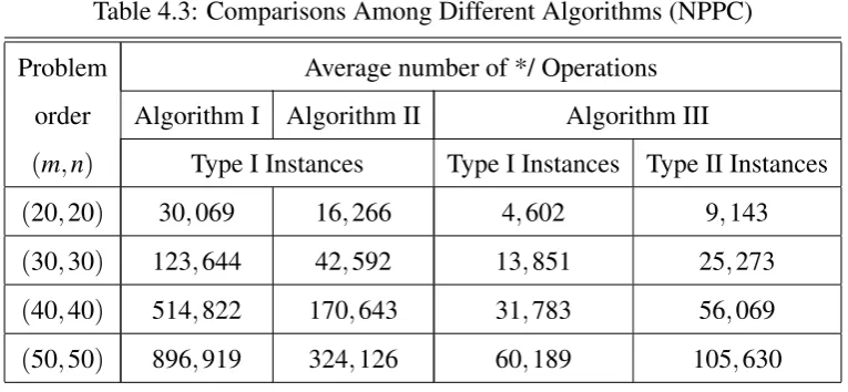
4.2.2 Number of basic operations . . . 59
4.2.3 Execution time . . . 62
4.3 Further Experiments . . . 69
4.3.1 Sparse matrices . . . 69
4.3.2 Numerical stability . . . 72
5 The Nearest Point Problem in A Polyhedral Set . . . 73
5.1 Methodology for Solving the Problem . . . 73
5.2 A Computational Experiment . . . 77
5.2.1 Data sets . . . 78
5.2.2 Results and observations . . . 79
6 Strictly Convex Quadratic Programming . . . 89
6.1 Methodology for Solving the Problem . . . 89
6.2 A Computational Experiment . . . 91
6.2.1 Data set . . . 91
6.2.2 Results and observations . . . 92
7 Conclusion and Future Research . . . 96
7.1 Overview of Accomplishments . . . 96
7.2 Future Research Directions . . . 97
LIST OF TABLES
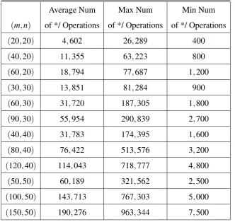
Table 4.1 Number of arithmetic operations for instances of type I (NPPC) . . . 56
Table 4.2 Number of arithmetic operations for instances of type II (NPPC) . . . 57
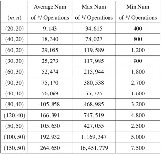
Table 4.3 Comparisons Among Different Algorithms (NPPC) . . . 59
Table 4.4 Number of basic operations for type I instances (NPPC) . . . 60
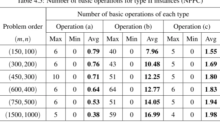
Table 4.5 Number of basic operations for type II instances (NPPC) . . . 61
Table 4.6 Comparison with Cplex 11 for type I instances of smaller size (NPPC) . . . . 63
Table 4.7 Comparison with Cplex 11 for type II instances of smaller size (NPPC) . . . 64
Table 4.8 Comparison with Cplex 11 for type I instances of larger size (NPPC) . . . 66
Table 4.9 Comparison with Cplex 11 for type II instances of larger size (NPPC) . . . 67
Table 4.10 Comparison with Cplex 11 for type I instances with sparse matricesd=0.2 (NPPC) . . . 70
Table 4.11 Comparison with Cplex 11 for type II instances with sparse matricesd=0.2 (NPPC) . . . 71
Table 5.1 Number of basic operations for type III instances (NPPS) . . . 80
Table 5.2 Number of basic operations for type IV instances (NPPS) . . . 81
Table 5.3 Comparison with Cplex 11 for type III instances of smaller size (NPPS) . . . 83
Table 5.4 Comparison with Cplex 11 for type IV instances of smaller size (NPPS) . . . 84
Table 5.6 Comparison with Cplex 11 for type IV instances of larger size (NPPS) . . . . 87
LIST OF FIGURES
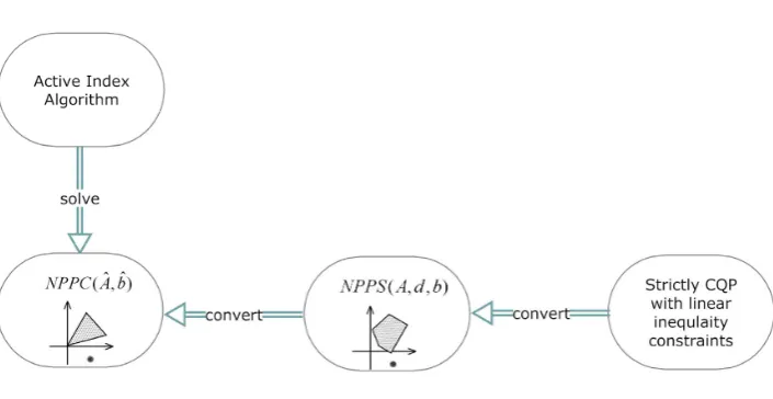
Figure 1.1 Application of the Active Index Algorithm . . . 3
Figure 1.2 The minimum distance between models . . . 8
Figure 3.1 Relationship betweenNPPC(A,b)and[b;pos(Γ)]. . . 32
Chapter 1
Introduction
In this dissertation we propose a new and efficient algorithm for solving the problem of finding the nearest point in a polyhedral cone to a given point inRn. Then we extend this algorithm to solve a similar problem in the context of a polyhedral set, and finally to solve the problem of minimizing any strictly convex quadratic objective function on a polyhedral set. We also carry out extensive computational experiments to demonstrate the effectiveness of our proposed algorithm for relatively large instances of the problems. Throughout this dissertation, for any matrixA, we denote itsithrow and jth column byAi· andA·j, respectively, and we useAT to denote its transpose.
1.1. Statement of the problem
minimize (x−b)T(x−b) subject to Ax≤0
(1.1)
We refer to this problem as the nearest point problem in a polyhedral cone, and denote it byNPPC(A,b).
If the rows of matrixAare linearly independent, the nearest point problem in a polyhe-dral coneNPPC(A,b)can be posed as a nearest point problem in a simplicial cone (as we shall discuss later in Section 3.2), and the critical index algorithm in [23] can be applied to solve the problem. If, however, the rows of matrixAare not linearly independent, then the problem is more difficult to solve.
Our focus in this research is to study the nearest point problem in a polyhedral cone NPPC(A,b) when the rows of matrix A are not (necessarily) linearly independent. We develop an efficient algorithm for solving the problem in this case, which we refer to as the active index algorithm.
Similarly, given anmbynmatrixA, a right hand side vectord∈Rm, and a pointb∈Rn, the problem of finding the nearest point in a polyhedral set P={x∈Rn:Ax≤d} to the given pointb, can be formulated as following CQP
minimize (x−b)T(x−b) subject to Ax≤d
(1.2)
We refer to this problem as the nearest point problem in a polyhedral set, and denote it by NPPS(A,d,b).
to convert an instance of the nearest point problem NPPS(A,d,b) into an instance of the nearest point problem NPPC(Aˆ,b), and then use our proposed active index algorithm toˆ solve this problem (as shown in Figure 1.1).
Finally we show that our proposed algorithm can be also used to solve any strictly convex quadratic programming problem with linear inequality constraints. To this end, we propose a methodology to convert an instance of the strictly convex quadratic programming problem into an instance of the nearest point problem NPPS(A,d,b), and then solve the problem using the methodology mentioned above (as shown in Figure 1.1).
1.2. Karush–Kuhn–Tucker conditions
Since the objective function in either problem,NPPC(A,b)orNPPS(A,d,b), is strictly convex, and the constraints are linear, it follows that the KKT conditions provide both necessary and sufficient conditions for optimality in either problem.
In (1.1), by dropping the constant term in the objective function of (1.1) and dividing it by 2, the problem is equivalent to
minimize 12xTx−bTx subject to Ax≤0
(1.3)
Then we can write the corresponding Lagrangian function as
g(u,x) = 1 2x
Tx+uTAx−bTx (1.4)
whereu∈Rm is the Lagrangian multiplier. Taking derivatives of the Lagrangian function (1.4) with respect tox, and setting that to zero, we have
x=b−ATu (1.5)
Substituting (1.5) into (1.4) and dropping the constant terms we have the following La-grangian dual of (1.3)
minimize 12uTAATu−bTATu subject to u≥0
(1.6)
x+ATu=b uTAx=0
Ax≤0 u≥0
(1.7)
We can rewrite these conditions as a linear complementarity problem as follows. Left-multiply the first equation of (1.7) by matrix−A, let−Ax=y, and substitute it into (1.7); then we have
y−AATu=−Ab uTy=0 u≥0,y≥0
(1.8)
(1.8) is a linear complementarity problem (LCP) with a special structure, in which the coefficient matrixAAT is positive semidefinite.
A similar development can also be done for the nearest point problem NPPS(A,d,b), leading to the following KKT conditions.
x+ATu=b uT(Ax−d) =0
Ax≤d u≥0
(1.9)
Again, the KKT conditions lead to the following LCP.
y−AATu=d−Ab uTy=0 u≥0,y≥0
On the other hand, since we can easily retrieve the solutions to the KKT conditions, (1.7) and (1.9), from the solutions to the LCPs, (1.8) and (1.10), respectively, it follows that existing algorithms for solving LCP can also be used to solve the nearest point problems NPPC(A,b) and NPPS(A,d,b). (Suppose (u∗,y∗) is a solution for either (1.8) or (1.10); then(u∗,x∗), wherex∗=b−ATu∗, is the corresponding solution to (1.7) or (1.9))
1.3. Applications of the problems
The nearest point problem in a polyhedral cone, the nearest point problem in a poly-hedral set, and the strictly convex quadratic programming problem with linear inequality constraints can arise in many contexts. Following are several specific applications of these problems.
1.3.1. Algorithm for Linear Programming Problem
In [25] a gravitational method that behaves like the interior point method for linear programming is proposed. In each iteration, it uses a new centering strategy that moves one interior feasible solution x0 to the center of the feasible region on the hyperplane of the objective function that passes through x0, before beginning the gravitational descent moves. The strategy makes the radius of the ball aroundx0 as large as possible. In [25], it is shown that this strategy leads to an algorithm for LP that terminates after a polynomial number of iterations.
1.3.2. Positive Linear Approximation Problems
LetΦbe a finite-dimensional function space, and letDbe the common domain of the functions inΦ. LetLbe a linear functional defined onΦ. For example,
L f =
Z
D
ω(x)f(x)dx, ω(x)≥0 (1.11)
where f ∈Φ. From [33], we know that there exist points x1,x2, ...,xN∗ inDand positive weightsλ1,λ2, ...,λN∗ so that
L f = N∗
∑
i=1
λif(xi) (1.12)
for all f ∈Φ. Given the linear functionalL, the positive linear approximation problem is to find such points and weights for (1.12).
Equation (1.12) is called a Tchakaloff representation for L. If T is a subset of D and there exists a Tchakaloff representation for L which uses points only in T, then T is called a Tchakaloff set. Letϕ1,ϕ2,...,ϕnbe a basis forΦ,M= (Lϕ1,Lϕ2, ...,Lϕn)T and e(x) = (ϕ1(x),ϕ2(x), ...,ϕn(x))T. Wilhelmsen [33] solves the positive linear approximation problem by solving the nearest point problem from the pointq=Mto the polyhedral cone generated by the point setE ={e(xi):xi∈T}, whereT is a finite Tchakaloff set. There is no assumption about the vectors in the setE, which means that the vectors inE may or may not be linearly independent. This problem is equivalent to the nearest point problem of the form (1.1) as we discuss later in Chapter 3 (Section 3.2).
1.3.3. Application in Robotics
of the shortest line segment between the objects (e.g. Figure 1.2). For non-convex objects, we can break each object into convex components and then determine the distance between those convex components ([28]).
Figure 1.2: The minimum distance between models
Consider the problem of finding the distance, d, between two compact and convex objects inRn,K1andK2. It follows thatdcan be written as following.
d=min{kzk ∈Rn:z∈K}, whereK=K1−K2 (1.13)
In Robotics,K1andK2are often two polytopes, denoted by
Kk={zk∈Rn:zk= Mk
∑
l=1
λlzkl,λl≥0,λ1+...+λl=1} (1.14) wherezkl, for k=1,2, andl=1,2, ...,Mk, are extreme points ofK1 andK2, respectively. Then it is easy to show thatK is the polytope
K={z∈Rn:z=
2
∑
k=1
Mk
∑
l=1
λklzkl,λkl≥0,
2
∑
k=1
Mk
∑
l=1
More details of this application can be found in [9].
1.3.4. Model Predictive Control
Consider a nonlinear dynamical system with control variables u, state variablesx, and outputsy, which is formulated as
dx
dt =φ(x,u) y=h(x,u)
(1.16)
The discrete time version of the above system can be written as
xt+1=xt+φ(xt,ut)∆t yt=h(xt,ut),t=1,2, ...,N
(1.17)
Given steady state pointsxs andus (i.e.φ(xs,us) =0), we linearize the nonlinear func-tionsφ andh; then the discrete time system can be written as
xt+1=xt+φx(xs,us)(xt−xs)∆t+φu(xs,us)(ut−us)∆t yt=h(xs,us) +hx(xs,us)(xt−xs)∆t+hu(xs,us)(ut−us)∆t t =1,2, ...,N
(1.18)
whereφxdenotes the Jacobian ofφ with respect tox, and so on.
In Model Predictive Control, the objective is to make the variables of the system track certain reference trajectories as closely as possible. Let Tty, Ttx, Ttu represent reference trajectories foryt,xt,ut, respectively, then we can formulate the objective as
min N
∑
t=1
yt−Tty
2 Wy+ N
∑
t=1kxt−Ttxk
2
Wx+ N
∑
t=1
kut−Ttuk
2
Wu (1.19)
kβkW =pβTWβ =
r
∑
i
wiiβi2 (1.20)
The diagonals of the weighting matrixW represent the relative weights of various objec-tives. In general, the weights are set such that the Hessian of the objective function, (1.19), is well conditioned and positive definite, i.e. there is unique optimal solution.
Normally, there are linear inequality constraints involving the variables, which can be expressed as
AU≤b (1.21)
whereU = [x1,y1,u1,x2,y2,u2, ...,xN,yN,uN]T.
Therefore, we can formulate the above Model Predictive Control problem as a strictly convex quadratic programming problem in the following form:
min 12UTHU+cTU s.t. AU ≤b
EU =r
(1.22)
where the equality constraints represent the linearized discrete time dynamical system, (1.18).
Let Z be a matrix whose columns form a basis of the null space ofE, and given any particular solution Up that satisfies EUp =r, then the general solution for the equality constraints can be written as
U =Up+Zx (1.23)
programming problem with only linear inequality constraints.
min p
1 2x
T(ZTHZ)x+ (c+HU p)TZx s.t. AZx≤b−AUp
(1.24)
More details of this application can be found in [6].
1.4. Contributions of This Research
In this research we propose an efficient algorithm to solve the nearest point problem in a polyhedral cone NPPC(A,b), and by extension to solve the nearest point problem in a polyhedral setNPPS(A,d,b), and the strictly convex quadratic programming problem with linear inequality constraints. In particular,
1. We show that the nearest point problemNPPC(A,b)is equivalent to a nearest point problem in a pos cone which is the polar cone (dual cone) of the polyhedral cone C={x∈Rn:Ax≤0}.
2. We show that if we know the index of an active constraint of the nearest point problem NPPC(A,b,d), the order (size) of the problem can be reduced by one.
3. We design a procedure to find the index of an active constraint of the nearest point problemNPPC(A,b).
4. We propose several strategies for efficient implementation of the algorithm.
6. We also extend our proposed algorithm to solve any strictly convex quadratic pro-gramming problem with linear inequality constraints.
7. We carry out an extensive computational study to show the efficiency of our proposed algorithm.
1.5. Outline of This Dissertation
The current chapter is followed by Chapter 2, in which we present a literature review on different methods for solving the nearest point problem in a polyhedral coneNPPC(A,b), the nearest point problem in a polyhedral setNPPS(A,d,b), and related problems, such as the convex quadratic programming problem and the linear complementarity problem.
In Chapter 3 we present our active index algorithm for solving the nearest point problem NPPC(A,b). First, we show that, given the index of one active constraint of problem (1.1), both the number of variables and the number of constraints can be reduced by one; Second, we show how to find the index of one active constraint of (1.1); Third, we propose several strategies for the efficient implementation of our algorithm.
In Chapter 4 we present the results of a computational experiment in which we evaluate the computational requirements of our proposed algorithm for the nearest point problem in a polyhedral coneNPPC(A,b).
In Chapter 5 and Chapter 6 we extend our proposed algorithm to solve the nearest point problem in a polyhedral set NPPS(A,d,b)and the strictly convex quadratic programming problem with linear inequality constraints, respectively. Computational results are also given in these two chapters to show the efficiency of our proposed algorithm.
Chapter 2
Literature Review
As we mentioned in Chapter 1, the nearest point problem in a polyhedral coneNPPC(A,b) and the nearest point problem in a polyhedral setNPPS(A,d,b)are special cases of the con-vex quadratic programming problem. There is a large body of literature that addresses the convex quadratic programming problem and a number of algorithms have been developed for solving this problem. In this chapter we give a brief review of the most prominent al-gorithms in this context that are applicable to the nearest point problems that we consider here. We divide these algorithms into three main categories.
1. Algorithms particularly designed for the nearest point problem in a polyhedral cone NPPC(A,b) and the nearest point problem in a polyhedral setNPPS(A,d,b)based on their special structures ([3], [23], [33], [35]).
2. Algorithms for the convex quadratic programming problem with linear constraints, such as active set methods ([16]), interior point methods ([21], [11], [2]), projection methods ([10], [12], [29]), and simplex methods ([32], [34]).
linear complementarity problems (LCP).
2.1. Special Algorithms
When row vectors of matrixAare linearly independent, from (1.8) we know that in this case the square matrixAAT in (1.8) is positive definite, and thus aP-matrix. In ([23]) Murty and Fathi propose an efficient algorithm for solving the nearest point problem in a given simplicial cone to a given point which is outside of the simplicial cone. They show that this problem is equivalent to an LCP with aP-matrix and propose a critical index algorithm for solving this problem. In particular, they consider the nearest point problem[Γ;b]in which Γ={A·1,A·2, ...,A·n}is a basis forRn,b∈Rnand it is required to find the nearest point in the simplicial conePos(Γ)tob(assumingb∈/Pos(Γ)).
Letx∗denote the nearest point inPos(Γ)tob, and letx∗= ∑n i=1
αiA·i. In [23] they define an indexito be acritical indexifαi>0. First, by using elementary row operations on the matrix of LCP, it is shown that given a single critical index of the LCP, the dimension of the problem can be reduced by one. Second, a subroutine is designed for finding a critical index by using the properties of the projection from a given point onto a simplicial cone.
Using the idea of polar cones that we describe in Section 3.2, we show that in this case the nearest point problem[Γ;b]is equivalent to a corresponding nearest point problem in a polyhedral coneNPPC(A,b)of the form that we consider. The key difference, however, is that the vectors by which the cone is generated may be linearly dependent in our algorithm, while they must be linearly independent in [23]. In our algorithm for finding the active index we also use the properties of the projection from a given point onto a cone which is similar to the simplicial cone.
origin to a polytope, which is the convex hull of a given point setP. The algorithm main-tains an affinely independent vector setQ, which is a subset ofP, and a pointX, which is in the convex hull ofQ. In each iteration, the algorithm updates the setQand the point X so that the distance from the origin toX is strictly reduced. The algorithm stops whenX =0 or the hyperplaneH(X) ={x:XT(X−x) =0}separatesPfrom the origin.
2.2. Convex Quadratic Programming
It is well known that the convex quadratic programming problem with linear constraints is inP(the class of problems solvable in polynomial time), and therefore there exist poly-nomial time algorithms that can be applied to solve this problem. Following is a brief description of four different polynomial algorithms for solving the convex quadratic prob-lem.
2.2.1. Active Set Methods
min q(x) = 12xTQx+bTx subject to aTi x=di,i∈E
aTi x≤di,i∈I
(2.1)
whereQis a symmetric positive semidefiniten×nmatrix, andE andI are finite sets of indices, which represent the equality constraints and inequality constraints, respectively. In iterationk, the primal active set methods find a moving direction, pk, fromxk toxk+1 by solving a quadratic subproblem, in which some of the inequality constraints of (2.1) and all the equality constraints are considered as equalities. This subset of constraints is referred to as aworking set. The gradientaiof the constraints in the working set are required to be linearly independent so that the equality-constrained quadratic subproblem can be easily solved by solving the KKT system. The process is continued until it finds xk that would minimize the quadratic subproblem over the subspace defined by the working set.
From the above description, we can see that the primal active set methods search for dual feasibility while maintaining primal feasibility and complementary slackness. In con-trast, the dual active set methods search for primal feasibility while maintaining dual feasi-bility and complementary slackness.
2.2.2. Interior Point Methods
Interior point (or barrier) methods are also known to be efficient for solving the convex quadratic programming problem, they are inspired by Karmarkar’s algorithm ([15]) for the linear programming problem. The basic idea of the interior point methods consists of a barrier function in the objective function to maintain strict feasibility of all iterations.
Monteiro and Adler ([21]) developed a primal-dual small-step path-following method for the convex quadratic programming problem which requires a total ofO(√nL)number of iterations and a total number of arithmetic operations of the order ofO(n3L), whereLis the input size. Each iteration updates a penalty parameter and finds an approximate Newton direction associated with the KKT system which characterizes a solution of the logarithmic barrier function problem.
Goldfarb and Liu ([11]) proposed a primal small-step logarithmic barrier method for the convex quadratic programming problem, which also requires a total ofO(√nL)number of iterations and a total number of arithmetic operations of the order ofO(n3L). This approach generates a sequence of problems each of which is approximately solved by taking a single Newton step.
Anstreicher, Hertog, Roos and Terlaky ([2]) proposed a long-step logarithmic barrier function method for the convex quadratic programming problem with linear equality con-straints. The total number of iterations isO(√nL)orO(nL), depending on how the barrier parameter is updated.
2.2.3. Projection-type Methods
within the linear complementarity and the variational inequality problems, of which the convex quadratic programming problem is a special case. These methods have a similar iterative scheme which solves a sequence of quadratic programming subproblems with the constraints of the original problem and an easy Hessian matrix.
Goldfarb and Idnani ([10]) presented a projection type dual algorithm for solving the convex quadratic programming problem. It uses the fact that the unconstrained minimum of the objective function can be also used as a starting point for the dual problem. A dual algorithm then iterates until primal feasibility is achieved, which is equivalent to solving the dual by a primal method. Numerical results show that the proposed dual algorithm is superior to primal algorithms when a primal feasible point is unavailable.
Han ([12]) proposed a successive projection method for finding the projection of a point on the intersection of a finite number of closed convex sets by a sequence of projections to the individual sets successively. The main feature of the method is to decompose the projection problem into several small ones.
2.2.4. Simplex Methods
In 1959, Wolfe ([34]) proposed the simplex method for the convex quadratic program-ming problem, which is inspired by the simplex method for the linear programprogram-ming prob-lem, and in 1960s interior point methods were discovered in the form of barrier function methods. In 1984, Karmarkar ([15]) formally proposed his interior point method for the linear programming problem. After that, interior point methods were much applied to non-linear programming models (including the quadratic programming problem), and few peo-ple focused on the simpeo-plex methods for the convex quadratic programming problem. Here, we briefly discussed the main ideas of Wolfe’s simplex methods for the convex quadratic programming problem.
Suppose that we consider the following convex quadratic programming problem,
min 12xTQx+bTx subject to Ax=d x≥0
(2.2)
whereQis symmetric positive semidefiniten×nmatrix, andd≥0. And then we can write the KKT conditions as the following.
Ax = d
Qx−v+ATu = −b
xTv = 0
x≥0,v≥0
(2.3)
Ax+w = d Qx−v+ATu+z1−z2 = −b x,v,z1,z2,w≥0
(2.4)
Sinced≥0, an initial basis for system (2.4) can be formed from the coefficients ofz1,z2,
andw. The method uses the simplex method for linear programming to minimize∑ i
wi(to zero), keepingvanduzeros. By discardingwand the unused components ofz1andz2, and
letting the remainingncomponents ofz1 andz2be denoted byZ and their coefficients by E, we have a basic solution of the system:
Ax = d
Qx−v+ATu+EZ = −b x,v,Z≥0
(2.5)
which also satisfies xTv=0. Given this basic solution to (2.5), the method makes one change of the basis in the simplex procedure for minimizing the linear function
n ∑ k=1
Zk, under the rule: ifxk is in the basis, do not admitvk, and ifvk is in the basis, do not admit xk. In this way, the method iteratively changes the basis of (2.5), until
n ∑ k=1
Zk=0, and then we have a solution to (2.3), which is also an optimal solution to (2.2).
2.3. GCPs and LCPs
Given a closed convex coneK ⊆Rn and its dual coneK∗={y∈Rn:yTx≥0, for all x∈K}, let f be a function from K toRn, the generalized complementarity problem is to find all solution vectorsxsuch that
x∈K, f(x)∈K∗ xT f(x) =0
(2.6)
To obtain (1.8), let K ={u∈Rn:u≥0}, and then K∗=K ={u∈Rn:u≥0}. Let f(u) =AATu−Ab, and then (1.8) can be considered as a special case of generalized com-plementarity problem in the form of (2.6). Similar development can also be applied to obtain (1.10).
In [7], Fang proposed an iterative method for solving the generalized complementarity problems, for which the linear complementarity problem is a special case. He proved that, under some conditions, the proposed iterative strategy generates a sequence of points which converges to the unique solution of the given generalized complementarity problem. Later in [8], he proposed a linearization method for solving the same set of problems.
Chapter 3
The Nearest Point Problem in A
Polyhedral Cone
In this chapter we propose a new algorithm for solving the nearest point problem in a polyhedral coneNPPC(A,b). We refer to this algorithm as the active index algorithm. To this end, we study the geometric structure ofNPPC(A,b)and its relationship with the near-est point problem in a pos cone, and employ this relationship at various levels in the design of our proposed algorithm. Finally we end this chapter by proposing several strategies for efficient implementation of the algorithm.
In Section 3.1 we describe a procedure by which we can reduce the order of the nearest point problem in a polyhedral coneNPPC(A,b)if we know an active index. In Section 3.2 we use the concept of polar cone to show that the nearest point problem in a polyhedral cone NPPC(A,b)is equivalent to an associated nearest point problem in a pos cone. In Section 3.3 we exploit this relationship to design a procedure to determine an active index, and in Section 3.4, we address the subject of efficient implementation of the proposed method.
3.1. Reducing the Order of the Problem
Consider the nearest point problem in a polyhedral coneNPPC(A,b), whereAis a given m×nmatrix andbis a given column vector of sizen. LetM={1, ...m}andN={1,2, ...,n}
represent the index sets of rows and columns of matrix A, respectively. LetAi· be the ith row of matrixAandx∗∈Rnbe the optimal solution for the problem. We refer to an index i∈M as an active indexifAi·x∗=0. The collection of all active indices is referred to as theactive setand it is denoted byI, i.e.,I={i∈M:Ai·x∗=0}.
For a given nearest point problem in a polyhedral coneNPPC(A,b)we define theorder of the problem as the size of matrixA, and denote it by(m,n).
The following theorem states that if we know one active index of the given nearest point problem in a polyhedral coneNPPC(A,b), we can reduce the order of the problem.
THEOREM3.1. If a single active index for the nearest point problem in a polyhedral cone NPPC(A,b)of order(m,n)is known, the problem can be reduced to another nearest point problem in a polyhedral cone of order(m−1,n−1).
we know thati∗is an active index, i.e.A
i∗·x∗=0. Without loss of generality, in the following discussion we assumei∗=1. Then we have
a11x∗1+a12x∗2+...+a1nx∗n=0. (3.1) We now make the following linear transformation.
x01=a11x1+a12x2+...+a1nxn x02=x2
.. . x0n=xn
(3.2)
By assumption there exists at least one index j∈N such thata1j6=0. Again without loss of generality we assumea116=0. Dividing both sides of the first equation bya11, we have
x1= a1
11x
0
1−
a12
a11x
0
2−...−
a1n a11x
0 n
x2=x02
.. . xn=x0n
(3.3)
In matrix form we can write (3.3) asx=Kx0, where
K= 1
a11 −
a12
a11 · · · −
a1n a11
0 1 · · · 0 ..
. ... . .. ... 0 0 · · · 1
is a nonsingular matrix. Substitutingx=Kx0into (1.1), we have minimize (b−Kx0)T(b−Kx0)
s.t x01 ≤0
a21(a1
11x
0
1−
a12
a11x
0
2−...−
a1n a11x
0
n) +a22x02 +... +a2nx0n ≤0 ..
. am1(a1
11x
0
1−
a12
a11x
0
2−...−
a1n a11x
0
n) +am2x02 +... +amnx0n ≤0
(3.4)
Note that(b−Kx0)T(b−Kx0) =bTb−2bTKx0+x0TKTKx0; by dropping the constant term, dividing it by 2, and writing it in matrix form, we conclude that (3.4) is equivalent to
minimize 12x0TJx0−b0Tx0
s.t. x01 ≤0
cx01+A(x¯ 02,x03, ...,x0n)T ≤0
(3.5)
whereb0=KTbis ann-vector,J=KTK is a square symmetric positive definite matrix of ordern,c= (a21
a11, ...,
am1
a11)
T is an (n−1)-vector, and
¯ A=
a22−a21a12
a11 · · · a2n−
a21a1n a11
..
. . .. ...
am2−ama111a12 · · · amn−ama111a1n
By assumption we know that at the optimal solution of problem (3.5) we have x01= 0. Substitutingx01=0 into (3.5), we observe that
x0TJx0=
h
0 x02 · · · x0n
i
j11 j12 · · · j1n j21 j22 · · · j2n
..
. ... . .. ... jn1 jn2 · · · jnn
0 x02
.. . x0n
and
b0Tx0=h b01 b02 · · · b0n
i 0 x02 .. . x0n
=b¯0Tx¯0 (3.7)
where ¯x0= (x02, ...,x0n)T and ¯b0=h b02 · · · b0n
iT
are (n−1)-vectors, and
¯ J=
j22 · · · j2n ..
. . .. ... jn2 · · · jnn
isn−1 byn−1 matrix. Therefore, given the fact that 1 is an active index, problem (1.1) is reduced to the following problem.
minimize 12x¯0TJ¯x¯0−b¯0Tx¯0 s.t. A¯x¯0≤0
(3.8)
SinceJ=KTK is symmetric positive definite matrix, it follows that ¯J is also a symmetric positive definite matrix. Hence there exists a nonsingular matrix ¯K such that ¯J =K¯TK¯ (For example, the Cholesky factor of ¯J)1. Lettingb00T =b¯0TK¯−1andx00=K¯x¯0we can now rewrite the objective function in (3.8) in the following equivalent form
min 12x¯0TJ¯x¯0−b¯0Tx¯0
⇔ min ¯x0TK¯TK¯x¯0−2b00TK¯x¯0+b00Tb00
⇔ min (b00−x00)T(b00−x00) Thus problem (3.8) is equivalent to
1In section 3.4 we propose an efficient procedure to determine the matrixKand its inverse using its special
minimize (b00−x00)T(b00−x00) s.t. A¯K¯−1x00≤0
(3.9)
It is clear that problem (3.9) has the structure of a nearest point problem in the polyhedral coneC00 ={x00 ∈Rn−1: ¯AK¯−1x00≤0}to the given point b00, which is of order(m−1,n−
1).
From the proof above it is evident that, if we have the optimal solution, say x00∗, to problem (3.9), the optimal solution to problem (1.1) is
x∗=K
0 ¯ K−1x00∗
(3.10)
In other words, we can retrieve the optimal solution to the nearest point problem (1.1) of order (m,n) given the optimal solution to the nearest point problem (3.9) of order (m−
1,n−1).
The following procedure summarizes the computational steps required to solve a given nearest point problem NPPC(A,b) of order (m,n), if we have an active index for this problem and a procedure to find the optimal solution of a corresponding problem of or-der(m−1,n−1).
Input: The data (A,b) and one active index of the nearest point problemNPPC(A,b), say i, 1≤i≤m.
Step one: Choose one nonzero element among the coefficients of the ith constraint, say that the jth element, 1≤ j ≤n; Go to step two. Without loss of generality, throughout the presentation we assume i=1 and j =1. Otherwise, we can rearrange the rows and columns of matrixAand the vectorbaccordingly.
step three.
Step three: Compute the matrix ¯K and its inverse; go to step four.
Step four: Compute b00 and solve the nearest point problem NPPC(A¯K¯−1,b00). Let the optimal solution bex00∗; go to step five.
Step five: Compute the optimal solution for the original problem according to (3.10). In step one, for reasons of numerical stability, if we have more than one nonzero ele-ments in the ith row, we always choose the nonzero element that has the largest absolute value.
Later in Section 3.4 we address the subjects of efficient implementation of these steps. In particular, we propose an efficient procedure to determine the matrix ¯K and its inverse using its special structure, and we discuss some issues related to the corresponding matrix multiplication operations.
3.2. The Polar Cone of the Polyhedral Cone
In the previous section we showed that given an active index, the order of the nearest point problem NPPC(A,b) can be reduced by one. In this section we show that finding an active index for the nearest point problemNPPC(A,b)is equivalent to finding acritical index(defined below) in a corresponding nearest point problem defined on apos conewhich is the polar coneof the polyhedral coneC={x∈Rn:Ax≤0}. To describe the method, we need to introduce a few definitions and lemmas.
DEFINITION 3.1. For any subset S⊆Rn, the polar cone of S, denoted by Sp, is the set
y∈Rn|yTx≤0, for all x∈S .
of rows of A. The pos cone generated by the rows of A, denoted by pos(Γ), is the set
{x∈Rn|x= ∑ i∈M
αiATi·,αi≥0}.
DEFINITION 3.3. Given a matrix A∈Rm×n and the corresponding collection of its rows Γ, the problem of finding the nearest point in pos(Γ) to a given point b is denoted by [b;pos(Γ)].
DEFINITION3.4. Let x∗be the optimal solution to the problem[b;pos(Γ)], an index i∈M is called a critical index in this context if Ai·(b−x∗) =0. In other words, i is a critical index if ATi· is orthogonal to b−x∗.
The following lemmas, taken from [30], establish the relationship between a polyhedral cone and its polar cone. We present these lemmas without proof.
LEMMA 3.1. The polyhedral cone C= {x ∈ Rn : Ax≤ 0} is equal to the polar cone (pos(Γ))p.
LEMMA 3.2. Given a cone K ⊆Rn, letK p represent its polar cone. Let b be a given point in Rn, x∗and x∗prepresent the nearest points inK andK p, respectively, to the given point b. Then x∗and x∗pare orthogonal to each other and b=x∗+x∗p.
From Lemma 3.1 and Lemma 3.2, we observe that if we can find the nearest point from bto pos(Γ), sayx∗p, then the nearest point frombto the the polyhedral coneC={x∈Rn: Ax≤0}, sayx∗, isb−x∗p, andx∗⊥x∗p.
we have the following proposition:
PROPOSITION3.1. Let the nearest point problem NPPC(A0,b0)be the subproblem of order (m−1,n−1) obtained from the nearest point problem NPPC(A,b) based on one active index, and letΓ0={A10T·,A02T·, ...,A0(m−T 1)·}. If b∈/ pos(Γ), then we have b0 ∈/ pos(Γ0).
Proof. Supposeb0 ∈pos(Γ0), it follows that the optimal solution of the nearest point prob-lemNPPC(A0,b0)is the 0. From (3.10), we know that the optimal solution of the nearest point problemNPPC(A,b)is also 0, and then we haveb∈pos(Γ), which is a contradiction. Therefore, given the fact thatbis not inpos(Γ),b0 cannot be inpos(Γ0)either.
Furthermore, based on Lemma 3.1 and Lemma 3.2, we have the following important result.
PROPOSITION 3.2. If index i is a critical index in the problem [b;pos(Γ)], then i is an active index in the corresponding nearest point problem NPPC(A,b).
Proof. Suppose the nearest points of the two problems[b;pos(Γ)]andNPPC(A,b)arex∗p andx∗respectively. From Lemma 3.1 and Lemma 3.2, we know that b=x∗p+x∗. Ifiis a critical index for the problem[b;pos(Γ)], thenb−x∗p is orthogonal toATi·. It follows that x∗=b−x∗pis also orthogonal toATi·, which implies thatAi·x∗=0, i.e.,iis an active index for the nearest point problemNPPC(A,b).
Proposition 3.2 shows us that, if we find a critical index for the problem [b;pos(Γ)], then we also find an active index for the nearest point problemNPPC(A,b). To make this clear, we give the following example, which is in two-dimensional space.
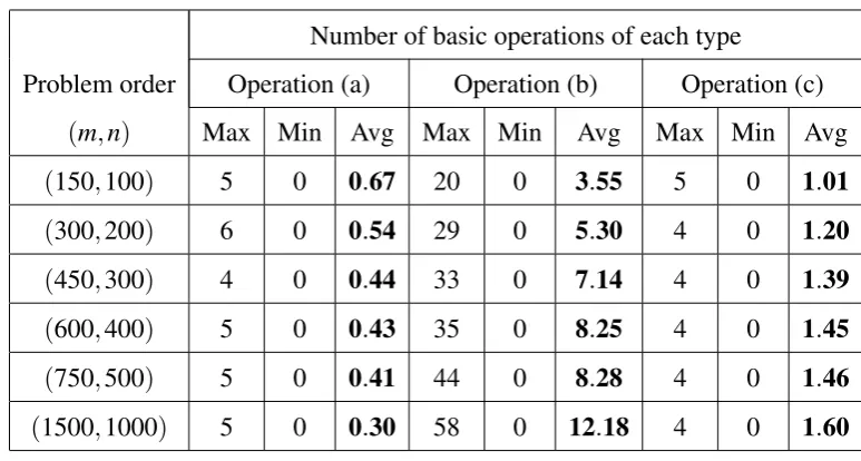
EXAMPLE3.1. In Figure 3.1, we have the polyhedral cone C={x∈R2:A1x≤0, A2x≤0}
Figure 3.1: Relationship betweenNPPC(A,b)and[b;pos(Γ)]
1. pos(Γ)is the polar cone of C.
2. x∗and x∗pare orthogonal to each other, and x∗+x∗p=b.
3. Index2is a critical index for the problem[b;pos(Γ)], and index2 is also an active index for the nearest point problem NPPC(A,b).
3.3. Finding a Critical Index for problem
[
b
;
pos
(
Γ
)]
assumed that the elements of the setΓare linearly independent, while here we remove this assumption and allow the elements ofΓ(i.e., rows of matrixA) to be linearly dependent.
Letting S= nATi
1·,A
T i2·, ...,A
T ir·
o
⊂Γ be a subset of the row vectors of matrix A, we define:
• I(S) =Index set ofS={i1,i2, ...,ir} • I(S) ={1,2, ...,m}\I(S)
• H(S) ={y:y= ∑ i∈I(S)
γiATi·;γireal number for alli∈I(S)}
• A(S) =Thenbyrmatrix whose columns areATi
1·,A
T i2·, ...,A
T ir·
• b(S) =The nearest point inH(S)tob.
Also let Smax be a maximal linearly independent subset of the vectors in S, ˆn be the cardinality ofSmax (obviously ˆn≤n), andA(Smax)be the corresponding nby ˆnmatrix of
these column vectors.
H(S) as defined above is the linear hull of S; Note that H(S) =H(Smax), and hence
b(S) =b(Smax). b(S)is known as the orthogonal projection ofbinH(S).
LetVibe the nearest point on the ray ofATi· tob. We have thatVi=0 ifAi·b≤0, and Vi=ATi·(Ai·b)/kAi·k2 ifAi·b>0. Also let l∈M={1,2, ...,m}be such thatVl−b
=
min{ Vi−b
:i∈M}.
Consider the hyperplaneT(b; ¯x) ={x:(x−x)¯ T(b−x) =¯ 0}. The open half space{x: (x−x)¯ T(b−x)¯ >0} is called the near side of T(b; ¯x), while the close half space {x: (x−x)¯ T(b−x)¯ ≤0} is called the far side of T(b; ¯x). If the point ¯x is chosen such that 0∈T(b; ¯x), then ¯xT(b−x) =¯ 0. Therefore, for such a point we have
• Near side ofT(b; ¯x) ={x:xT(b−x)¯ >0} • Far side ofT(b; ¯x) ={x:xT(b−x)¯ ≤0}
For ¯xsuch that 0∈T(b; ¯x), we defineN(x) =¯ {i:i∈MandAi·(b−x)¯ >0};N(x)¯ is the collection of indices of the vectors ATi· that are on the near side ofT(b; ¯x). The following results from [23] are used in the development of the procedure that we propose in this section.
LEMMA3.3. Let S be a subset of the rows of A, Smaxbe the maximum linearly independent
subset of S, and we assume that S6= /0. Then
b(S) =b(Smax) =A(Smax)(A(Smax)TA(Smax))−1A(Smax)Tb (3.11)
Note that the most efficient way to determine b(S) is to start multiplication from the right of the expression and proceed to the left. The corresponding computational require-ment is of orderO(nn).ˆ
LEMMA 3.4. If Vl=0, the nearest point in pos(Γ)to b is 0.
LEMMA 3.5. A pointx is the nearest point in pos(Γ)¯ to b if and only if 0∈T(b; ¯x) and Ai·(b−x)¯ ≤0, for all i∈M.
LEMMA 3.6. Letx¯∈ pos(Γ)be such that0∈T(b; ¯x). If there exists an index i∈M such that Aj·(b−x)¯ ≤0, for all j∈M\{i} and Ai·(b−x)¯ >0, then i is a critical index for problem[b;pos(Γ)].
LEMMA 3.7. Given 0 6=x¯∈ pos(Γ) satisfying 0∈T(b; ¯x), if for some i ∈M, we have Ai·(b−x)¯ >0andkb−x¯k ≤b−Vi
, where x and A¯ Ti· are linearly independent, then the
We are now prepared to describe our proposed procedure, which is called procedure CI, for finding a critical index of the nearest point problem[b;pos(Γ)]. Clearly, ifVl=0, the nearest point in pos(Γ)to bis just the origin. Therefore, in the following description we assume thatVl6=0. Throughout the procedure we maintain a nonempty subset ofΓcalled thecurrent set, denoted byS, and a maximum linearly independent subset ofS, denoted by Smax. The procedure also maintains a point called thecurrent point , denoted by ¯x; at all
time ¯x∈ pos(Smax). Following is a description of various steps of the procedure.
Procedure CI:
Initial step: Set ¯x=Vland computeN(x)¯ (See Remark 1). IfN(x) =¯ /0, then ¯xis the near-est point in pos(Γ)to b, by Lemma 3.2 we can easily determine the nearest point for the problemNPPC(A,b)and terminate this procedure. IfN(x)¯ is a singleton set, say k1, then k1is a critical index for the nearest point problem[b;pos(Γ)], by Proposition 3.2k1is also an active index for the nearest point problemNPPC(A,b), terminate this procedure. If the cardinality ofN(x)¯ is greater than or equal to 2, selectg∈N(x)¯ and compute the orthogonal projection, say ˆb, ofbonto the linear hull of{x¯,ATg·}. Replace ¯xby ˆb. SetS=Smax={ATl·,
ATg·}, compute the matrix(A(Smax)TA(Smax))−1, and go to step 1. (See Remark 2)
Step 1: ComputeN(x). If¯ N(x) =¯ /0, then ¯xis the nearest point in pos(Γ)tob; by Lemma 3.2 we can easily determine the nearest point for the problem NPPC(A,b) and terminate this procedure. IfN(x)¯ is a singleton set, sayk1, thenk1 is a critical index for the nearest point problem[b;pos(Γ)], hence k1 is also an active index for the nearest point problem NPPC(A,b), terminate this procedure. If the cardinality ofN(x)¯ is greater than or equal to 2, go to step 2 ifN(x)¯ ∩I(S)6= /0, or to step 3 ifN(x)¯ ∩I(S) =/0. (See Remark 3)
in Smax, replace Smax by Smax∪ {ATg·}, S by S∪ {ATg·}, and ¯x by ˆb, update the matrix (A(Smax)TA(Smax))−1 (See Remark5), and go back to step 1. If ATg· is linearly depen-dent with the vectors in Smax and ˆb∈ pos(Smax), Smax remains unchanged, replace S by
S∪ {ATg·}, and ¯x by ˆb, go back to step 1. Otherwise, if ATg· is linearly dependent with the vectors in Smax and ˆb∈/ pos(Smax), find a vectorATk· in Smax, such that the vectors in
{ATg·} ∪Smax\{ATk·}are linearly independent and ˆb∈pos({ATg·} ∪Smax\{ATk·}), replaceSmax
by{ATg·} ∪Smax\{ATk·},SbyS∪ {ATg·}, and ¯xby ˆb, update the matrix(A(Smax)TA(Smax))−1,
and go back to step 1. (See Remark 6)
Step 3: Computeb(Smax), the projection ofbonto the linear hull ofSmax. Go to step 4.
Step 4: Ifb(Smax) =bandb(Smax)∈pos(Smax), it follows thatb∈pos(Γ)and the
near-est point in pos(Γ) tobisbitself, terminate the algorithm. Ifb=6 b(Smax)andb(Smax)∈
pos(Smax), then b(Smax) is also in pos(S), replace ¯x byb(Smax)and go back to step 1. If
b(Smax)∈/ pos(Smax), go to step 5.
Step 5: Let the current point ¯x=∑(αjATj·: j∈I(Smax)), whereαj≥0 for all j∈I(Smax).
Letb(Smax) =∑(γjATj·: j∈I(Smax))(See Remark 7). Sinceb(Smax)∈/ pos(Smax), we have γj <0 for some j ∈I(Smax). Any point on the line segment joining ¯x to b(Smax)can be
written as
Q(λ) =
∑
[(1−λ)αj+λ γj]ATj·: j∈I(Smax),0≤λ ≤1Asλ increases from 0 to 1,Q(λ)moves from ¯xtob(Smax). Letλ be the largest value for
whichQ(λ)is in pos(Smax). So,Q(λ)is on the boundary of pos(Smax), and λ =max{λ :(1−λ)αj+λ γj≥0, for all j∈I(Smax)}
Letkbe such that(1−λ)αk+λ γk=0. If there is more than one index inI(Smax)with this
property, choose one of them arbitrarily. Then we haveQ(λ)∈pos(Smax\{ATk·}). Delete
ATk· from Smax and S, and update the matrix (A(Smax)TA(Smax))−1. Let ¯x=Q(λ). Test
vectors inSmax. If yes, let Smax={ATg·} ∪Smax, update the matrix(A(Smax)TA(Smax))−1,
and go back to step 4. Otherwise, go back to step 3. (See Remark 8)
REMARK 1. We computeN(x)¯ according to the definition, N(x) =¯ {i:i∈M andAi·(b−
¯
x)>0}. Every time that we update the current point ¯x,N(x)¯ is computed correspondingly. REMARK2. If termination does not occur in the initial step, after this step we havekb−x¯k<
b−Vl
and this property will continue to hold in all subsequent steps, sincekb−x¯knever
increases in the procedure.
REMARK 3. Every time the procedure visits step 1 we have 0 ∈ T(b; ¯x), and thus the conditions of Lemma 3.5 through Lemma 3.7 are satisfied.
REMARK4. The current point ¯xis always inpos(Smax)andkb−x¯knever increases. Since
Ag·T is always chosen fromN(x)¯ andkb−x¯k<kb−Vgk, by Lemma 3.7, it follows that the orthogonal projection of b on the linear hull of {ATg·,x¯} is also in the relative interior of pos({ATg·,x¯}).
REMARK 5. Every time the setSmaxis changed, we need to update the matrix
(A(Smax)TA(Smax))−1. Normally, the computational effort required to carry out this task
is of order O(nnˆ2), where ˆn=|Smax|. However, in Section 3.4.4 we propose an
updat-ing procedure to compute this inverse matrix based on the previous information, and the corresponding computational requirement is of orderO(nn).ˆ
REMARK6. In step 2, ifATg·is linearly dependent with the vectors inSmaxand ˆb∈/pos(Smax),
we can always choose an indexk∈I(Smax)such that{Ag·T} ∪Smax\{ATk·}is a set of linearly
independent vectors and ˆb∈ pos({ATg·} ∪Smax\{ATk·}). In Section 3.4.3 we address this issue and propose an efficient procedure to carry out the computation.
REMARK 8. In step 5, after ATk· is deleted from Smax and S, if we find an index g in I(S\Smax) such that ATg· is linearly independent with the vectors in Smax, the orthogonal projection of b on the linear hull of Smax, i.e., b(Smax), remains unchanged after ATg· is added to Smax, thus the procedure moves back to step 4. In this case, however, the coef-ficients γj of b(Smax) in terms of the vectors in Smax change (since the set of vectors in
Smaxis modified). We use the updated information of(A(Smax)TA(Smax))−1to computeγj according to (3.11).
Discussion:
Figure 3.2: Flow Chart of the Procedure CI
terminate after a finite number of steps. To see this we make the following observations.
1. The loop step 1→ step 2 → step 1 must terminate after at most m iterations and the procedure either terminates or moves to step 3, followed by step 4. At this step it either finds a projection face of pos(Γ) and moves back to step 1 or it moves to step 5. Every time the procedure goes to step 1 (either from step 2 or from step 4), the distance kb−x¯k strictly decreases, and at every other step this distance either decreases or remains the same.
2. Every time the procedure leaves step 5 the cardinality of the setS(and possibly the setSmax) decreases by 1. Thus the loop step 4→step 5→step 4 or step 4→step 5→
step 3→step 4 must terminate after at most|S| −2 visits to step 5, and the projection pointb(Smax)falls into the relative interior of pos(Smax), i.e., the procedure finds a
projection face of pos(Γ). This, in turn, leads the procedure back to step 1.
3. Since the cone pos(Γ)has only a finite number of projection faces (i.e., the setΓhas only a finite number of subsets), and since each projection face that we find in step 4 is strictly closer than all previous projection faces, it implies that the procedure must terminate after a finite number of steps.
3.4. Strategies for Efficient Implementation
In this section we propose several strategies for efficient implementation of the algo-rithm that we outlined above. These strategies are based on the mathematical properties and relationships among various entities, and we show that through these strategies the computational efficiency of the algorithm can be improved significantly. Note that|Smax|
and the number of variables are denoted by ˆnandn, respectively, and ˆn≤n.
3.4.1. Decomposition matrix
K
¯
and its inverse
In the context of Theorem 3.1, in order to construct a smaller nearest point problem of order (m−1,n−1), we need to construct a decomposition matrix ¯K(and its inverse) for the given (n−1)-dimensional square positive definite symmetric matrix ¯J such that ¯J=K¯TK.¯ The Cholesky decomposition method is an option to do this. However, the computational effort required to determine the Cholesky factor of ¯J is of order O(n3). In this section we propose an alternative method to compute the matrix ¯K and its inverse such that the computational requirement is of orderO(n2).
From (3.6) and the definition of the matrix K, it follows that ¯J=k¯k¯T +I, where I is the identity matrix of order (n−1), and ¯k= [k1,k2, ...kn−1]T = [−aa1211,· · ·,−aa111n]T. Our
proposed method is based on this special structure of the matrix ¯J.
Since ¯J is a symmetric positive definite matrix, there exists an orthogonal matrix P such that ¯J=PΛPT, whereΛis a diagonal matrix with all positive entries (eigenvalues of
¯
J) on the diagonal. Thus we have ¯J=PΛ12Λ12PT = (Λ12PT)T(Λ12PT), and it follows that
¯
K = (Λ12PT) and ¯K−1=PΛ− 1
2. In this section we show how to compute the orthogonal
LEMMA 3.8. The eigenvalues of the matrixJ¯=k¯k¯T+I areλ1=1with multiplicity n−2
andλ2=
n−1
∑ j=1
k2j+1with multiplicity1.
Proof. By assumption we have ¯k6=0, and thus the matrix ¯kk¯T is of order 1. It follows that|J¯−λ1I|=
k¯k¯T
=0, and the dimension of the null space of ¯kk¯T isn−1−1=n−2.
Therefore,λ1=1 is an eigenvalue of ¯J with multiplicity ofn−2. Furthermore, it is easy
to show that |J¯−λ2I|=0. Therefore, λ2 = n−∑1 j=1
k2j +1 is also an eigenvalue of ¯J with multiplicity of(n−1)−(n−2) =1.
Given the eigenvalues λ1 and λ2 as defined in Lemma 3.8, let the linearly
indepen-dent eigenvectors forλ1be{α1,α2, ...,αn−2}and the eigenvector forλ2be{αn−1}, where αi∈Rn−1 fori=1,2, ...,n−1. It follows that{α1,α2, ...,αn−2,αn−1}is a linearly
inde-pendent set andαn−1is orthogonal to all vectors in the set{α1,α2, ...,αn−2}. We can use
the Gram-Schmidt orthogonalization procedure on{α1,α2, ...,αn−2}to get a set of unit
or-thogonal vectors{β1,β2, ...,βn−2}and letβn−1= kααn−n−11k. ThenP= [β1,β2, ...,βn−2,βn−1]
is the orthogonal matrix we desire. However, the computational work of the general Gram-Schmidt procedure is of order O(n3). In the following we show how to choose the eigenvectors such that the computational requirement of the Gram-Schmidt proce-dure is of order O(n2). Without loss of generality, we assume that k1,k2, ...,ki 6=0 and ki+1=ki+2=...=kn−1=0, for somei, 1≤i≤n−1.
LEMMA 3.9. For j=1,2, ...,i−1, let αj be a vector of size n−1 such that its jth and (j+1)th elements are kj+1 and −kj, respectively, and all the other elements are zeros. For j =i,i+1, ...,n−2, let αj be such that its (j+1)th element is 1 and all the other elements are zeros. And let αn−1= [k1,k2, ...,kn−1]T. Thenαj, for j =1,2, ...,n−2, are linearly independent eigenvectors of J for¯ λ1 =1 and αn−1 is the eigenvector of J for¯ λ2=
n ∑ j=2
Proof. For j=1,2, ...,n−2, it is easy to show that(J¯−λ1I)αj=0 and theα0jsare linearly independent. Hence,α0js, for j=1,2, ...,n−2, are linearly independent eigenvectors of ¯J
for λ1=1. Furthermore, it is easy to show that(J¯−(
n−1
∑ j=1
k2j+1)I)αn−1=0. Therefore, αn−1is the eigenvector of ¯Jforλ2=
n ∑ j=2
k2j+1.
PROPOSITION3.3. The computational requirement of the Gram-Schmidt orthogonal pro-cedure on the vectors{α1,α2, ...,αn−2}defined in Lemma 3.9 is of order O(n2).
Proof. Note that, for j=1,2, ...,i−1,αjis orthogonal to all the other vectors in{α1,α2, ..., αn−2}exceptαj−1andαj+1, and for j=i, ...,n−2,αjis the unit vector and orthogonal to all the other vectors in{α1,α2, ...,αn−2}. Therefore, the Gram-Schmidt procedure is:
β1=kαα11k β2= β
0
2
kβ20k,whereβ
0
2=α2−(α2Tβ1)β1
.. .
βi−1=
βi−0 1
kβi−0 1k,whereβ
0
i−1=αi−1−(αi−T1βi−2)βi−2 βi=αi
βi+1=αi+1
.. .
βn−2=αn−2
(3.12)
From (3.12) we can see that the computational work for eachβj is of orderO(n), for j= 1,2, ...,i−1, and of orderO(1), for j=i,i+1, ...,n−2. Therefore, the total computational requirement of the Gram-Schmidt procedure is of orderO(n2).
¯
J=k¯k¯T +I=
5 −6 2 0
−6 10 −3 0
2 −3 2 0
0 0 0 1
First, according to Lemma 3.9, we have the corresponding eigenvectors of matrixJ,¯
α1 α2 α3 α4
−3 −2 0 0 0 1 3 0 0 0 0 1 2 −3 1 0
Next, according to Proposition 3.3, we use the Gram-Schmidt orthogonal procedure on the above eigenvectors, then we have
β1= kαα11k =
h
−0.8321 −0.5547 0 0
iT
β2=
β20
kβ20k =
h
−0.1482 0.2224 0.9636 0
iT
,whereβ20=α2−(α2Tβ1)β1
β3= α3 =
h
0 0 0 1
iT
β4= kαα44k =
h
0.5345 −0.8018 0.2673 0
iT
Then we have
P=
−0.8321 −0.1482 0 0.5345
−0.5547 0.2224 0 −0.8018 0 0.9636 0 0.2673
0 0 1 0
On the other hand, from Lemma 3.8, we know that the eigenvalues of J are¯ λ1=1 and λ2=15. Then we have the diagonal matrix Λ
1
2, the matrixK¯ = (Λ 1
2PT), and its inverse
¯
K−1=PΛ−12.
From Lemma 3.8, Lemma 3.9, and Proposition 3.3, the total computational requirement for computing the orthogonal matrixPis of orderO(n2), and hence the total computational work required to compute ¯K and ¯K−1 is also of order O(n2). The following is a detailed procedure for computing ¯Kand ¯K−1.
Input:k¯= [k1,k2, ...kn−1]T.
Step 1: Let the nonzero elements of{k1,k2, ...kn−1} be denoted by {kj1,kj2, ...,kji}, and let the zero elements be denoted by {kji+1,kji+2, ...,kjn−1}, where j1 < j2 < ... < ji and ji+1< ji+2< ... < jn−1, and j1,j2, ...,jn−1∈ {1,2, ...,n−1}. Construct the eigenvectors
of matrixI+k¯k¯T, denoted byα1,α2, ...,αn−1, as follows: Forr=1,2, ...,i−1,letαjr be a vector of sizen−1 such that the jthr element iskjr+1, the j
th
r+1element is−kjr and all the
other elements are zeros. Forr=i,i+1, ...,n−2, letαjr be such that the jthr+1element is 1
and all the other elements are zeros. Letαn−1= [k1,k2, ...kn−1]T.
βj1 =
αj1
kαj1k
βj2 =
β0j
2 β 0 j2
,whereβ0j
2 =αj2−(α
T
j2βj1)βj1
.. .
βji−1 =
β0ji−
1 β 0 ji−1
,whereβ0ji−1=αji−1−(α
T
ji−1βji−2)βji−2
βji =αji
βji+1 =αji+1
.. .
βjn−2=αjn−2
βn−1= kααn−1
n−1k
ThenP= [β1,β2, ...,βn−1].
From the procedure above, we can see that the primary computational effort of this procedure is in step 2, and by Proposition 3.3 this computational effort is of orderO(n2). Therefore, the total computational work required to compute ¯K and ¯K−1is of orderO(n2).
3.4.2. Matrix multiplication
By computational experiments we notice that one of the time-consuming operations of our proposed algorithm is matrix multiplication. Note that the only matrix multiplication appears in the order reduction step of our proposed algorithm, which is ¯AK¯−1in (3.9).
In (3.9), matrix ¯Acan be a full dense matrix, while, from the construction procedure of ¯
× × × · · · × × × × × · · · × ×
0 × × · · · × ×
0 0 × · · · × ×
..
. ... . .. ... ... ...
0 0 0 0 × ×
where×means nonzero element. Therefore, the computational requirement of the multi-plication between ¯Aand ¯K−1could be less than that of the multiplication between two full dense matrices. However, if we multiply ¯Aand ¯K−1 in a naive way (strictly according to the definition of matrix multiplication), this operation still takes a lot of time in our active index algorithm.
In the implementation of our active index algorithm, we use the Intel Math Kernel Li-brary (MKL) to carry out the matrix multiplications. The MKL contains the Basic Linear Algebra Subroutines, which reduce the computational requirements of matrix multiplica-tion fromO(n3)toO(n2.376). This results in some reduction in the execution time of our proposed algorithm.
3.4.3. Finding
A
Tk·in step 2 of procedure CI
In step 2 of procedure CI, if ATg· is linearly dependent with the vectors in Smax and
ˆ
b∈/pos(Smax), and we need to find an indexk∈I(Smax)such that{ATg·}∪Smax\{ATk·}is a set of linearly independent vectors and ˆb∈pos({ATg·}∪Smax\{ATk·}). In this section we propose an efficient method to find such an index. For ease of presentation, in the following two Lemmas we use the notationa1,a2, ...,anˆto represent the collection of linearly independent
earlier.
LEMMA 3.10. Given a collection of linearly independent vectors, a1,a2, ...,anˆ ∈Rn and
an+ˆ 1∈Rnsuch that
an+ˆ 1=α1a1+α2a2+...+αnˆanˆ (3.13)
whereα1,α2, ...,αnˆ∈R, ifαk6=0for some k∈ {1,2, ...,nˆ}, then the collection of the vectors a1,a2, ...,ak−1,ak+1, ....,anˆ,an+ˆ 1is linearly independent.
Proof. Suppose a1,a2, ...,ak−1,ak+1, ....,anˆ,an+ˆ 1 are linearly dependent, then there exist γ1,γ2, ...,γk−1,γk+1, ...,γn+ˆ 1not all zeros such that
γ1a1+γ2a2+...+γk−1ak−1+γk+1ak+1...+γnˆanˆ+γn+ˆ 1an+ˆ 1=0 (3.14)
andγn+ˆ 1must be nonzero (Otherwisea1,a2, ...,anˆ are linearly dependent). Dividing (3.14)
byγn+ˆ 1, it follows that
an+ˆ 1=β1a1+β2a2+...+βk−1ak−1+βk+1ak+1...+βnˆanˆ (3.15)
From (3.13) and (3.15), we have
(α1−β1)a1+ (α2−β2)a2+...+ (αk−1−βk−1)ak−1+
αkak+ (αk+1−βk+1)ak+1...+ (αnˆ−βnˆ)anˆ=0
(3.16)
Sinceαk6=0, (3.16) implies thata1,a2, ...,anˆ are linearly dependent, which is a
contradic-tion.
LEMMA 3.11. Given a collection of linearly independent vectors, a1,a2, ...,anˆ ∈Rn, and
a pointx¯∈ pos(a1,a2, ...,anˆ), suppose we have another vectoran+ˆ 1 ∈Rn such that an+ˆ 1
is linearly dependent witha1,a2, ...,anˆ, and the orthogonal projection of b onto the linear
hull of{x¯,an+ˆ 1}, denoted byb, is in pos(ˆ x¯,an+ˆ 1). Ifbˆ∈/ pos(a1,a2, ...,anˆ), then there exists
(i)a1,a2, ...,ak−1,ak+1, ....,anˆ,an+ˆ 1are linearly independent,
and
(ii)bˆ∈ pos(a1,a2, ...,ak−1,ak+1, ....,anˆ,an+ˆ 1).
Proof. First, given thatan+ˆ 1is linearly dependent witha1,a2, ...,anˆ, we have
an+ˆ 1=α1a1+α2a2+...+αnˆanˆ (3.17)
where α1,α2, ...,αnˆ ∈R. Second, we can always choose one index k such that αk 6=0. Dividing both sides of equation (3.17) byαkand rearranging the terms, it follows that
ak=−
α1
αk a1−
α2
αk
a2−...− αk−1
αk
ak−1− αk+1
αk
ak+1−...− αnˆ
αk anˆ+
1
αk
an+ˆ 1 (3.18)
From Lemma 3.10 we know thata1,a2, ...,ak−1,ak+1, ....,anˆ,an+ˆ 1are linearly independent.
Furthermore, since ¯x∈pos(a1,a2, ...,anˆ)and ˆb∈pos(x¯,an+ˆ 1), we have
¯
x=γ1a1+γ2a2+...+γnˆanˆ (3.19)
ˆ
b=θ1an+ˆ 1+θ2x¯ (3.20)
whereγi≥0 for alli, and θ1,θ2≥0. Then by substituting for ak from (3.18) into (3.19) and for ¯xfrom (3.19) into (3.20) we have
ˆ
b=θ2(γ1−αα1kγk)a1+θ2(γ2−αα2kγk)a2+...+θ2(γk−1−ααk−k1γk)ak−1
+θ2(γk+1−ααk+1k γk)ak+1+...+θ2(γnˆ−ααkjγk)anˆ+ (θ1+θ2αγkk)an+ˆ 1
(3.21)
Therefore, to guarantee that ˆb∈pos(a1,a2, ...,ak−1,ak+1, ....,anˆ,an+ˆ 1), we need to find an

![Figure 3.1: Relationship between NPPC(, A) b and [ b; pos() ] Γ](https://thumb-us.123doks.com/thumbv2/123dok_us/1599225.1197516/43.595.175.433.109.363/figure-relationship-nppc-b-b-pos-g.webp)