Abstract
WALKER, CARRIE L. Neutron Capture Measurements on 97Mo with the DANCE Array.
(Under the direction of Gary Mitchell and Undraa Agvaanluvsan.)
Neutron capture is a process that is crucial to understanding nucleosynthesis, reactors, and nuclear weapons. Precise knowledge of neutron capture cross-sections and level densities is necessary in order to model these high-flux environments. High-confidence spin and parity as-signments for neutron resonances are of critical importance to this end. For nuclei in the A=100 mass region, the p-wave neutron strength function is at a maximum, and the s-wave strength
function is at a minimum, producing up to six possible Jπ combinations. Parity
determina-tion becomes important to assigning spins in this mass region, and the large number of spin
groups adds complexity to the problem. In this work, spins and parities for 97Mo resonances
are assigned, and best fit models for photon strength function and level density are determined.
The neutron capture-cross section for97Mo is also determined, as are resonance parameters for
Neutron Capture Measurements on 97Mo with the DANCE Array
by
Carrie L. Walker
A dissertation submitted to the Graduate Faculty of North Carolina State University
in partial fulfillment of the requirements for the Degree of
Doctor of Philosophy
Physics
Raleigh, North Carolina
2013
APPROVED BY:
Gary Mitchell
Chair of Advisory Committee
Undraa Agvaanluvsan Co-chair of Advisory Committee
Mohammed Bourham Christopher Gould
Biography
Acknowledgements
First, I want to say thanks to all the other DANCE experimentalists who welcomed me into the group and gave me a place to learn. John Ullmann and Aaron Couture – you guys have been immensely helpful to me every step of the way. Thank you, Milan Krticka, for all your assistance with DICEBOX modeling. Your talents in this field are unparalleled, and I deeply appreciated the input and expertise you’ve offered.
A very special thanks to Bayar, who, over the course of several years, has been a constant guide and occasional sounding board in this long process. I believe that only google has fielded more question from me than you!
Another special thank you to Undraa, who took me under her wing and really went above and beyond to show me new opportunities and encourage my curiosity. I have always admired and been inspired by the passion for what you do and your ability to communicate it so enthu-siastically to others.
I also want to thank those people who have inspired and supported my education since it’s early days. Thanks, Mr. Reidy, for being the coolest stinking science teacher ever! Your knowledge, enthusiasm and candor lit up those long, boring days at OHS. Thank you, Dr. Maung, Dr. Mead, and Dr. Whitehead for guiding and pushing me in my study of physics at USM. You guys really never failed me, and I can’t begin to tell you how useful all your instruction has been! Dr. Gearba: thank you for taking time to introduce me to research. I made mistakes of all kinds, but you encouraged me to keep going. That meant a lot to me. I’d also like to express my deep gratitude to Dr. Hannelore Giles and the late Dr. William Giles, who supported my undergraduate education through their generous contributions to the USM Presidential Scholarship program.
On a very personal note, I’d like to thank all my special loved ones. My parents, who have always offered their unconditional love. Mary Alice, Lindsey, Nancy, Megan, Brittney, Paula, Kaycee, Georgina, for all your emotional support. Thanks, Toby and Sierra, for lifting my spirits in the worst of times. And especially Bryan, my best friend, my better half – thanks for letting me lean on you. I love you all!
Table of Contents
List of Tables . . . vi
List of Figures . . . vii
Chapter 1 Introduction . . . 1
Chapter 2 Theory. . . 3
2.1 Compound Nuclear Reactions . . . 3
2.2 R-Matrix Framework . . . 3
2.2.1 Resonance Reactions . . . 4
2.3 Statistical Models of Nuclear Reactions . . . 5
2.3.1 Hauser Feshbach Theory . . . 5
2.4 Level Density . . . 6
2.4.1 Constant Temperature Model . . . 6
2.4.2 Back-Shifted Fermi Gas Model . . . 7
2.5 Photon Strength Functions . . . 7
2.5.1 Single Particle Model . . . 8
2.5.2 Brink-Axel Model . . . 8
2.5.3 Kadmenskij, Markushev and Furman Model . . . 8
2.5.4 Generalized Lorentzian Model . . . 9
Chapter 3 Experimental Techniques and Data Processing . . . 10
3.1 The LANSCE Facility and DANCE . . . 10
3.2 Data Acquisition . . . 13
3.3 Data Reconstruction . . . 14
3.4 Background Subtraction . . . 16
Chapter 4 Spin and Parity Assignments . . . 23
4.1 Previous methods . . . 23
4.1.1 Average Multiplicity . . . 23
4.1.2 Oak Ridge Method . . . 25
4.1.3 Prague Method . . . 25
4.2 Method of Pattern Recognition . . . 26
4.2.1 Simple case: two spin groups . . . 27
4.2.2 Parity Assigments . . . 29
4.2.3 Results of s-wave resonances . . . 31
4.2.4 Generalization to p-wave case . . . 32
4.2.5 Results of p-wave resonances . . . 32
Chapter 5 Neutron Capture Cross-Section and Resonance Parameters . . . 37
5.1 Cross Section Calculation . . . 37
5.1.1 Neutron Flux . . . 37
5.1.3 Cross Section Results . . . 41
5.2 Resonance Parameters . . . 42
Chapter 6 Photon Strength Function and Level Density Parameters . . . 46
6.1 Simulation of γ-ray Cascades . . . 46
6.1.1 DICEBOX Code . . . 46
6.1.2 GEANT4 Simulations . . . 48
6.2 Previous Calculations . . . 48
6.3 Photon Strength Function for98Mo . . . 48
6.4 Level Density . . . 54
Chapter 7 Conclusions. . . 59
List of Tables
Table 3.1 Molybdenum Target: Isotopic Composition . . . 17
Table 4.1 Spins, Parities of Neutron Resonances . . . 33
Table 5.1 Resonance Parameters for97Mo as fit by SAMMY . . . 42
List of Figures
Figure 3.1 Layout of the Lujan Center and its flight paths. . . 10
Figure 3.2 Layout of flight path 14 and DANCE. . . 11
Figure 3.3 Neutron flux (neutrons/cm2/eV/To) at the DANCE detector. . . 12
Figure 3.4 A cross-sectional view of DANCE. . . 12
Figure 3.5 A waveform and its extracted parameters. . . 13
Figure 3.6 Timeline of a beam spill. . . 14
Figure 3.7 A contour plot of fast versus slow component integrals of signals. Integral units are arbitrary. Events inside the red gates are α particles. . . 15
Figure 3.8 Anαfit used forγ-ray energy calibrations for a single crystal. Histogram shows counts per energy bin, where the energy units are arbitrary. . . 16
Figure 3.9 Time card deviations over the duration of experiment for multiple crys-tals. Channel offsets in ns are plotted versus run number. . . 17
Figure 3.10 Capture counts per neutron energy bin, with and without summed-energy gate from 8.20 to 9.20 MeV, including multiplicies 3 and higher. . . 18
Figure 3.11 Summed energy spectra (MeV) sorted by multiplicity. . . 19
Figure 3.12 Multiplicity two summed energy spectra (MeV) from before (blue) and after (black) scattering subtraction. The iron data are shown in red. . . . 20
Figure 3.13 Multiplicity three summed energy spectra (MeV) from before (blue) and after (black) scattering subtraction. Iron data shown in red. . . 21
Figure 3.14 Counts per neutron energy bin before (black) and after (blue) scattering background subtraction using binwise estimation. . . 22
Figure 4.1 Average multiplicity of s-wave resonances. . . 24
Figure 4.2 Average multiplicity of p-wave resonances. . . 27
Figure 4.3 Two overlapping Gaussian distributions. . . 28
Figure 4.4 M5 vs M3 distributions for s-wave resonances . . . 29
Figure 4.5 Multiplicity twoγ-ray spectra for s- and p-wave resonances. . . 30
Figure 4.6 Capture yield contribution by spin group for some s-wave resonances. . . 31
Figure 4.7 Multiplicity 5 versus multiplicity 3 distributions for p-wave resonances. . . 32
Figure 4.8 Capture yield contribution by spin group for some p-wave resonances. . . 36
Figure 5.1 Cross Section of the197Au resonance used to normalize the neutron flux. . 38
Figure 5.2 Neutron flux measured at DANCE over the duration of the97Mo experi-ment. . . 39
Figure 5.3 Fractional effect of beam attenuation and target self-shielding as a func-tion of neutron energy. . . 40
Figure 5.4 Cross section determined for97Mo. . . 41
Figure 5.5 Experimental cross-section fit using SAMMY. . . 45
Figure 6.2 Comparison of the two E1 PSF parameterizations from the TLO model of Rusev et al. and that suggested by Berman. The curves are nearly indistinguishable. . . 49
Figure 6.3 Eγspectra from two nuclear realizations using the E1(GLO) and M1(SP+SF)
PSF model for a 2+ resonance. Multiplicities 1 through 7 are shown; the
last histogram is summed over all multiplicities. . . 50
Figure 6.4 Esumspectra from two nuclear realizations using the E1(GLO) and M1(SP+SF)
PSF model for a 2+ resonance. Multiplicities 1 through 7 are shown; the
last histogram is summed over all multiplicities. . . 51
Figure 6.5 Eγspectra from two nuclear realizations using the E1(GLO) and M1(SP+SF)
PSF model for a 2− resonance. Multiplicities 1 through 7 are shown; the
last histogram is summed over all multiplicities. . . 52
Figure 6.6 Esumspectra from two nuclear realizations using the E1(GLO) and M1(SP+SF)
PSF model for a 2− resonance. Multiplicities 1 through 7 are shown; the
last histogram is summed over all multiplicities. . . 53
Figure 6.7 Data from Oslo, Rossendorf and Saclay (“ 98Mo”, “ 98Mo
renormal-ized”) shown with parametrization from GLO, SLO, and Oslo models. The proposed GLO model agrees well with reasonably well with all but the Rossendorf data. . . 54
Figure 6.8 Comparison of experimental and simulated Eγ spectra for Jπ = 2+. The
BSFG (gray area) and CT (black lines) models are used. Multiplicities 1
through 7 are shown; the last histogram is summed over all multiplicities. 56
Figure 6.9 Comparison of experimental and simulated Eγ spectra for Jπ = 3+. The
BSFG (gray area) and CT (black lines) models are used. Multiplicities 1
through 7 are shown; the last histogram is summed over all multiplicities. 57
Figure 6.10 Comparison of experimental and simulated Eγ spectra for Jπ = 2−. The
BSFG (gray area) and CT (black lines) models are used. Multiplicities 1
Chapter 1
Introduction
The modeling of nuclear reactions for energy and defense applications requires knowledge of nuclear cross sections, some of which are difficult to measure experimentally. These must be calculated using theoretical models, such as those implementing Hauser-Feshbach theory. Both nuclear level densities and photon strength functions are key components of calculated cross sections for nuclear reactions, and they must be known for a broad range of isotopes and nuclear temperatures.
The calculation of nuclear level densities relies in part on high-confidence spin and parity assignments for neutron resonances. Spin determination for many nuclei can be problematic, particularly for those in the mass range of A = 100. The centrifugal potential barrier typically
suppresses the formation of resonances with angular momentum higher thanℓ= 0. However, for
nuclei in this mass region the p-wave neutron strength function is at a maximum, and the s-wave strength function is at a minimum. As a result, the expected number of p-wave resonances is
roughly equal to the number of s-wave resonances. There are then six possible Jπ combinations to
consider: s-wave resonances can have two different spin values, and p-wave resonances up to four spin values. Given this complication, determining the parity of resonances is also particularly important. The spins and parities of many documented resonances in this mass region are unknown, and current nuclear data libraries often disagree in cases where assignments do exist. Thus there is a need for spin and parity assignment methods that improve upon existing results. After neutron capture, an excited nucleus commonly decays to its ground state by
se-quentially emitting several γ rays. Parity and angular momentum must be conserved for each
transition, and the emitted radiation is primarily E1, M1, or E2, in accordance with Weisskopf estimates. The spin and parity of the capture state influences the cascade pattern, specifically the “multiplicity” of the cascade, or the number of transitions emitted to reach the ground state.
The multiplicity of γ rays for a nuclear cascade can then provide information as to the spin
well-suited for measuring multiplicity distributions and for assigning resonance spins. DANCE is a
highly segmented 4π γ-ray calorimeter array located at the Los Alamos Neutron Science Center
(LANSCE), which provides a white beam of spallation neutrons for experiments. At DANCE
the full Q-value of the reaction is detected with high efficiency, while detailedγ-ray multiplicity
information is preserved, as well as individual γ-ray energy and time-of-flight information.
Distinguishing s-wave resonances from p-wave resonances historically has proven proved to be a difficult task. Resonances whose strengths fall between the expected values for s- and p-waves are particularly hard to assign. This ambiguity in parity assignments is dealt with
using simulations of γ decay with the Monte Carlo code DICEBOX. Spectra from γ decay
are simulated using details from a combination of known nuclear levels and levels which are artificially generated from level density (LD) and photon strength function (PSF) models. The
γ-ray spectra from two-step cascades in particular can give strong indications of the parity of
the resonance.
Once the parities of resonances have been determined, a statistical approach is employed
to analyze γ-ray multiplicity distributions for spin assignments. For each resonance, the
nor-malized experimental yields for each multiplicity constitute an N-dimensional vector, where N is the total number of multiplicities considered. In this multi-dimensional “multiplicity space,” the vectors fall into localized clusters, one per spin group. Using the well-known method of pat-tern recognition, probability density functions (PDFs) are extracted to make spin assignments. This statistical approach offers many advantages over previous methods. This method offers im-proved sensitivity over those using only average multiplicities by utilizing all of the multiplicity distribution information. It even offers advantages over some newer methods by eliminating the need to rely on a prototype resonance to determine an ideal multiplicity distribution for each spin group. This feature allows for variations in distributions due to both Porter-Thomas fluctuations and experimental error. The explicit use of a PDF also provides quantification of the certainty of assignments.
Experimental data from 97Mo is examined, where six Jπ combinations for resonances are
possible. The task of separating p-wave spin groups pushes the limits of the computational capability of this method, but given large enough sample sizes, high-confidence spin assign-ments can be extracted for roughly half of the resonances. For the rest of the resonances, two possible spin values can be assigned. In addition, LD and PSF model parameters have been
determined. Experimentally obtained γ-ray spectra have a complex dependence on both the
LD and the PSFs. Recovering these parameters from experiment is not straightforward. Several combinations of both the LD and the PSFs are explored until optimum parameters from best
fit models are obtained. Additional resonance parameters such as Γγ and Γn are also extracted
Chapter 2
Theory
2.1
Compound Nuclear Reactions
The physical theory describing nuclear reactions varies with the type and energy of the particles involved. In general, reactions can be categorized as either direct or compound. In direct reac-tions, the incident neutron passes through nucleus for a short time, only long enough to interact with one or a few nucleons. In the case of a compound reaction, the impinging particle thermal-izes with the other nucleons of the target, creating a compound nucleus in an excited state. The compound nucleus has no “memory” of how it was formed; thus the mode of its formation and the mode of its decay are independet. This assumption is referred to as the Bohr hypothesis. Interaction times for compound reactions are much longer than those of direct reactions.
The excitation energy of the compound nucleus is equal to the neutron separation energy of the newly formed nucleus plus the kinetic energy of the incoming neutron. The compound nucleus may then decay by means of multiple channels available to it. In the absence of particle
emission or fission, the nucleus transitions to an intermediate state by emitting aγ ray. In this
way multipleγ rays may be emitted before the nucleus reaches its ground state. This series of
γ rays emitted is sometimes referred to as theγ-ray cascade.
2.2
R-Matrix Framework
R-Matrix theory is a convenient framework for dealing with many nuclear reactions. The as-sumptions underlying R-Matrix theory are as follows:
1. Nonrelativistic quantum mechanics are valid for the system, i.e., HΨ = EΨ, where the
2. All processes in which more than two product nuclei are formed are ignored.
3. All processes of creation or destruction are ignored (most importantly, the creation or destruction of photons.)
4. Any two nuclei can be separated by some finite distance ac beyond which neither nucleus
experiences any polarizing potential field from the other.
The collision matrix U is defined as the amplitude of the outgoing waves in channel c’ that results from the unit-sized flux of collision in channel c. The channel notation c specifies all the
particles in the channel, including all quantum numbers describing them. The cross sectionσcc′
is then proportional to |Uc′c|2.The U matrix is both unitary and symmetric,
U†U = 1 (2.1)
Up,q=U−q,−p =Uq,p (2.2)
following conservation of probability and time-reversal symmetry.
The matrix U depends on energy E. “External” interactions, or those in the regions of
incoming or outgoing channels, are represented by the diagonal matrices L and Ω.“Internal”
interactions, or those occuring inside the compound nucleus, are represented by the non-diagonal
matrix R. The division between these two regions is denoted by the nuclear radius ac. This
divison is justified because the nuclear radius is reasonably well defined due to the short range
of nuclear forces. The choice of ac imposes boundary conditions on the nuclear wave functions,
giving rise to resonances in the reaction cross section. The R-matrix is given by the equation
Rcc′ = X
λ
γλ,c′γλ,c
(Eλ−E)
, (2.3)
whereλdenotes a compound nuclear state or energy level.γl,λis the reduced width amplitude.
γ2
l,λ is referred to as the reduced width of the energy level Eλ. Neitherγλ nor Eλ depend on the
energy of the incoming or outgoing channels.
γ2l,λ= ¯h2/(2mR)[ul,λ(R)]2 (2.4)
2.2.1 Resonance Reactions
the Breit-Wigner formula
σcc′(E) =
π k2
α
ΓcλΓc′λ
(E−Eλ)2+ 1/4Γ2λ
, (2.5)
where E is the incident energy, Γc,λ and Γc′,λare partial widths of the resonance in the entrance
and exit channels, and Γλ is the total width, which is equal to the sum of the partial widths
over all channels:
Γλ =
N X
c=1
Γc,λ, (2.6)
If the level width Γ is larger than the level spacing D of the nucleus, then the levels will over-lap strongly. The R-matrix formalism is thus especially convenient when investigating neutron capture within energy regions containing well-isolated resonances.
2.3
Statistical Models of Nuclear Reactions
2.3.1 Hauser Feshbach Theory
When examining aspects of reactions that are not limited to well-isolated resonances, an ap-proach using transmission coefficients is convenient. Hauser-Feshbach theory provides this kind of formulation for reactions that involve contributions from a large number of compound nuclear states. Assuming that the Bohr assumption is still valid, the cross section for a reaction channel can be written as a product of its formation (or, fusion) cross-section and the probability that it will decay into the exit channel b
σab=σaPb. (2.7)
Assuming time-reversal invariance of the system, then the reaction cross section will satisfy the following relation
ka2σab =k2bσba, (2.8)
where σba is the cross section of the inverse reaction. This principle is often referred to as the
principle of detailed balance. By introducing the transmission coefficient
Ta= 1−|Uaa¯|2, (2.9)
then the compound reaction cross section in the spinless case may be written as
σabHF = π
k2
a
(2l+ 1)PTaTb γTγ
. (2.10)
be applied to account for the probability of the channel having a total spin of s given its constituents. The generalized cross section becomes
σabHF = π
k2
a X
J,π
(2J+ 1)
(2I+ 1)(2i+ 1)
TaTb
,
X
γ
Tγ, (2.11)
where I is the spin of the target nucleus, i is the spin of the projectile, and J is total angular
momentum sum of i+I+ℓ. When concerned with (n,γ) reactions, the transmission coefficients
are typically treated as the product of two components, the photon strength functionfXL(Eγ)
and the level density ρ(E, J).
2.4
Level Density
The level density of a nucleus, and in this case of the compound nucleus, is defined as the number of energy levels within a given interval of energy. Theoretically, the level density of the nucleus could be calculated if all the eigenvalues of its Hamiltonian were known. However, this is only possible for the simplest of nuclear models. In practice, nuclear level densities are determined experimentally. At low excitation energies, the energy levels of the nucleus are spaced at intervals much larger than the widths of the states themselves. As excitation energy increases, the number of levels increases, and eventually the nuclear levels are no longer well separated. This region is referred to as the continuum region, and the level density function
ρ(E) = dN(E)
dE (2.12)
can be described using various models, where N(E) is the cumulative number of levels below an excitation energy E.
2.4.1 Constant Temperature Model
One such model is the Constant Temperature Formula. In this model the nucleus is treated as a Fermi gas with a fixed temperature and chemical potential. In terms of the particle number A and system energy E, the level density takes the form
ρ(E, J) = f(J)
T e
(E−Eo)/T, (2.13)
where T is the nuclear temperature and Eo is the energy backshift. f(J) is a statistical spin
distribution factor that denotes the probability that a randomly chosen energy level has spin J
whereσc is the spin cutoff parameter. Based on empirical evidence, σc has the form
σc= 0.98A0.29, (2.15)
where A is the mass number of the nucleus.
2.4.2 Back-Shifted Fermi Gas Model
The constant temperature formula may be augmented by considering the fact that fermions
tend to form pairs. This pairing energy can be included by introducing a shift E1 in the nuclear
excitation energy. This model is referred to as the Back-Shifted Fermi Gas (BSFG) and alters the spin cutoff parameter in the following way
σc2= 0.0888A2/3pa(E−E1), (2.16)
where a and E1 are adjustable parameters that are fit using experimental level densities found
at low excitation energies for that nucleus.
Von Egidy [1] suggested simplifying the spin cutoff parameter to
σc2= 0.391A0.675(E−P a′)0.312. (2.17)
2.5
Photon Strength Functions
The other component of the transmission coefficient is the photon strength function, sometimes referred to as the radiative strength function. The photon strength function (PSF) is related to the average partial radiation width from an initial state i to a final state f
hΓXLγifi= fXL(Eγ)E
2L+1
γ )
ρ(Ei, Ji, πi)
, (2.18)
2.5.1 Single Particle Model
The simplest model for the E1 PSF is the single particle model. This model does not depend on energy
fESP1 =CA
2/3
Ds
, (2.19)
where C = 6.8 x 10⁻⁸ MeV−2 and D
s is the spacing of ℓ= 0 single particle states.
2.5.2 Brink-Axel Model
A more realistic model incorporates the existence of the giant electric dipole resonance (GEDR)
observed in (γ,n) experiments. The GEDR can be understood as being caused by the
collec-tive dipole vibration of proton and neutron fluids within the nucleus. Brink hypothesized that the nature of the resonance was independent of excitation energy. Consequently, any photon strength function would not be a function of excitation energy, only of the energy of the
transi-tion. Assuming this hypothesis holds true, the principle of detailed balance for (γ,n) and (n,γ)
reactions allows the PSF for the GEDR to be written
fE1(Eγ) =
1 3(π¯hc)2
σ0EγΓ2G
(E2
γ−EG2)2+Eγ2Γ2G
, (2.20)
where σ0 is the peak cross section of the GEDR, EG is the peak position of the GEDR, and
ΓG is its full width at half maximum. This model is referred to as either the Brink-Axel or the
standard Lorentzian model (SLO). It begins to fail at energies near the neutron binding energy and also at low energies (1 - 2 MeV.)
2.5.3 Kadmenskij, Markushev and Furman Model
Another PSF model was proposed by Kadmenskij, Markushev and Furman (KMF) which is based on the theory of Fermi liquids (i.e., strongly interacting fermions.) The PSF is given by
fKM FE1 (Eγ, T) =
1
3(π¯hc)2(0.7)
σ0EGΓGΓ(Eγ, T)
(E2
γ−EG2)2
. (2.21)
Unlike the SLO model, the KMF model is temperature dependent; the strength function
depends not only on the energy of theγ ray but also the excitation energy of the nucleus. This
2.5.4 Generalized Lorentzian Model
Introduced by Kopecky and Chrien [2], the generalized Lorentzian (GLO) model modifies the
KMF model by removing the divergence as Eγ→ EG.
fGLOE1 (Eγ, T) =
1
3(π¯hc)2(0.7)σ0ΓG
"
EGΓ(Eγ, T)
(E2
γ−EG2)2+Eγ2Γ2(Eγ, T)
+ (0.7)4π
2T2Γ
G
E2
G #
Chapter 3
Experimental Techniques and Data
Processing
3.1
The LANSCE Facility and DANCE
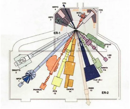
Figure 3.1: Layout of the Lujan Center and its flight paths.
Exper-iments (DANCE.) The center houses a linear accelerator which produces both positive and negative hydrogen ions and accelerates them to energies of up to 800 MeV. A proton storage ring (PSR) strips the ions and bunches them into 250 ns-wide pulses before they are injected into the Mark-III neutron spallation target at a rate of 20 Hz. The spallation target, located in the Lujan Center, is made of two cylinders of natural tungsten surrounded by light water and liquid hydrogen moderators. Each proton impinging on the target produces up to 17 neutrons. Beryllium reflectors push the neutron energy flux further into the thermal region. Neutrons then travel radially outward down various flight paths in the Lujan Center to be used for experiments (see Figure 3.1.)
Figure 3.2: Layout of flight path 14 and DANCE.
DANCE is located on flight path 14 (see Figure 3.2.) The flight path length for neutrons is approximately 20.3 m. Flight times of neutrons through the aluminum beam pipe range from hundreds of ns to 14 ms. Collimators are installed on FP14 to reduce the beam size to approximately 70 mm in diameter. The neutron flux at FP14 varies with accelerator operations and the performance of the spallation target. The typical flux distribution at DANCE is shown in Figure 3.3.
DANCE itself is a nearly 4π γ-ray calorimeter (see Figure 3.4.) The detector array comprises
160 BaF2 scintillator crystals forγ-ray detection, each crystal subtending an equal solid angle.
Each crystal is 15 cm long and 734 cm3 in volume. Holes in the sphere allow for the entry and
exit of the beam pipe. Targets are inserted via the beam pipe into the center of the array and kept under vacuum (0.05 torr) for the duration of data collection. Surrounding the beam pipe is
a 6 cm-thick shell of6LiH which serves to absorb scattered neutrons with minimal attenuation
of γ rays.
The high γ detection efficiency of BaF2 and the large solid angle coverage ensure that
essentially all γ rays from a nuclear cascade are detected. The total efficiency of DANCE for
Figure 3.3: Neutron flux (neutrons/cm2/eV/To) at the DANCE detector.
reliable measurement of the γ-ray multiplicity of the cascade. Scintillation signals from BaF2
contain a fast and a slow component, providing information on both event timing and the total
energy deposited. The energy resolution of BaF2 is less than that of other scintillators but is
suffient to distinguish individual γ rays and measure the summed energy of each cascade.
3.2
Data Acquisition
Each crystal’s light output is collected by its own PMT and split into two digitizer channels. The
digitizers are triggered by a To coming from the PSR beam burst plus a delay. Each channel
records event information from the crystal over a set timing window. Together the channels
typically cover 500 µs of looking time, corresponding to neutron energies of 8.5 eV to 2 MeV.
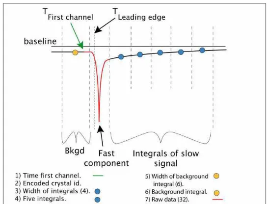
The digitizers are capable of sampling at 500 MHz with 8-bit resolution and have 128 kb of fast memory. Since full utilization of the sampling rate would lead to data rates exceeding hundreds of TB per day, only fundamental parameters of the waveforms are extracted and written from each beam burst (see Figure 3.5). A constant fraction discriminator is used to identify events in a crystal. The following quantities are then recorded for each crystal event: a 100 ns-wide integral of the background baseline before the event; 32 points at the maximum sampling rate covering the leading edge of the event (the fast component); five 200 ns-wide integrals of the slow component, giving total energy deposition information; and two time stamps, one relative
to a master clock and one relative to the beam pulse trigger To.
Figure 3.5: A waveform and its extracted parameters.
It takes about 40 ms to read out the digitizers, process the waveforms and write the com-pressed event information to a network RAID. The digitizers are rearmed in time for the next beam pulse, which comes every 50 ms. A time line of acquisition for each beam spill is shown in Figure 3.6.
Figure 3.6: Timeline of a beam spill.
schemes for data acquisition have been utilized at DANCE and have been described elsewhere. The double continuous mode was the only mode implemented for the experiments discussed in this work.
3.3
Data Reconstruction
During offline analysis, physics events from each beam spill are reconstructed from the com-pressed data. Time stamps from each crystal signal within a narrow coincidence window (50
ns) are identified as one physics event. γ-ray cascades alone are not responsible for all physics
events;α radiation originating in the crystals themselves is a significant source of background.
Since radium is a chemical homologue of barium, there are traces of it within the BaF2. Several
isotopes of radium are α emitters. α particle events are distinguishable from γ-ray events by
examining the relative amount of energy deposited in the fast component and slow component
integrals of the scintillation signal.α particles deposit a greater fraction of their energy in the
slow component of the signal than γ rays do. Also, the α-particles are emitted with discrete
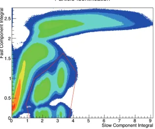
energies, while theγrays are emitted with a continuous distribution of energies (see Figure 3.7).
Thus a well-chosen gate on the ratio of the two components removesαparticle events from the
experimental data set.
Once only γ-ray events are left, the time stamp of the event relative to the trigger To
corresponds to the time-of-flight of the incident neutron. The energy of the neutron is calcu-lated using the estimated flight path length and later is fine-tuned by fitting the time-of-flight spectrum to existing resonance data.
Many crystals fire during one physics event. However, the number of crystals fired may far
Figure 3.7: A contour plot of fast versus slow component integrals of signals. Integral units are
arbitrary. Events inside the red gates areα particles.
in multiple adjacent crystals via Compton scattering. Thus the notion of cluster multiplicity is introduced. When multiple adjacent crystals fire within the same physics event, the energy
de-posited in the cluster is attributed to oneγ ray. The cluster multiplicity, not crystal multiplicity,
then serves as a more accurate measure of the γ-ray multiplicity of the cascade.
Energy calibrations of the crystals were made by using knowledge of the naturalα
radioac-tivity within the crystals. The α particles emitted originate from the 226Ra and 228Ra decay
chains and have well-known, discrete energies. The energy peaks measured from theα particles
were fit with a sum of five Gaussians. The resulting position of each gaussian’s center corre-spond to known energies. The correlation of the known energies to the signal integrals are fit with a simple linear relation using these points.
E(x) =a+b∗x (3.1)
These constants were generated for each crystal on a run-by-run basis. A sample of theseα
fits is provided in Figure 3.8.
Alpha_043
Entries 5867
Mean 1.839e+04
RMS 4445
10000 15000 20000 25000 30000
0 20 40 60 80 100 120 140 160 180
Alpha_043
Entries 5867
Mean 1.839e+04
RMS 4445
Alpha_043
Figure 3.8: An α fit used for γ-ray energy calibrations for a single crystal. Histogram shows
counts per energy bin, where the energy units are arbitrary.
digitizer channels are not perfectly aligned in time when data is recorded. Time stamps from each channel typically differ by less than 20 ns. In order to set a more narrow coincidence window and further reduce backgrounds, it is necessary to perform time calibrations for all the
channels. Time stamps from allγ-ray cascade events are collected within a run, and the average
time stamp was calculated. The deviation of each channel’s average from an arbitrarily chosen reference channel was calculated, and then applied as a corrective offset. The offsets for each channel are plotted in Figure 3.9 and illustrates how the channel timings are relatively stable over the course of the experiment.
3.4
Background Subtraction
The high total efficiency of the DANCE calorimeter allows selection of events with summed
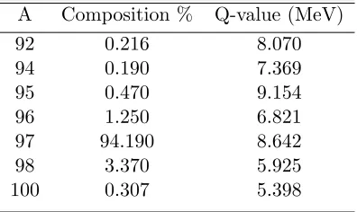
energies near the Q-value of the desired reaction. The Q-value of the 97Mo(n,γ) reaction is
8.642 MeV. The target used for capture measurements is a self-supporting foil of molybdenum
enriched to 94.190% in 97Mo. The isotopic composition of the target is shown in Table 3.1.
Those isotopes with significantly lower Q-values than that of 97Mo will not have large
contributions in the data as long as the summed energy threshold is set above those Q-values.
The only isotope that presents a problem in the analysis is95Mo, whose Q-value is only 512 keV
26380 26400 26420 26440 26460 26480 -30 -20 -10 0 10 20 30 Crys 60 Crys 61 Crys 62 Crys 63 Crys 64 Crys 65 Crys 66 Crys 67 Crys 68 Crys 69 Time Dev
26380 26400 26420 26440 26460 26480
-30 -20 -10 0 10 20 30 Crys 70 Crys 71 Crys 72 Crys 73 Crys 74 Crys 75 Crys 76 Crys 77 Crys 78 Crys 79 Time Dev
Figure 3.9: Time card deviations over the duration of experiment for multiple crystals. Channel offsets in ns are plotted versus run number.
Table 3.1: Molybdenum Target: Isotopic Composition
A Composition % Q-value (MeV)
92 0.216 8.070
94 0.190 7.369
95 0.470 9.154
96 1.250 6.821
97 94.190 8.642
98 3.370 5.925
100 0.307 5.398
95Mo cannot be separated by a Q-value gate alone. While95Mo makes up only a small fraction
of the target mass, its thermal cross section is approximately six times higher than that of
97Mo. Nonetheless, contributions from 95Mo should be largely negligible, except near strong
95Mo resonances. The strongest resonances from 95Mo are indeed visible in the capture data,
but only at energies far from the resonances of interest. By applying a summed-energy gate of 8.20 to 9.20 MeV, signal-to-noise is improved by a factor of 10 (see Figure 3.10).
Neutron Energy [eV]
20 40 60 80 100 120 140 160
Counts per bin
10
2
10
3
10
4
10
5
10
6
10
Counts per Neutron Energy Bin
M<=2, ungated M<=3, Q-gated
Figure 3.10: Capture counts per neutron energy bin, with and without summed-energy gate from 8.20 to 9.20 MeV, including multiplicies 3 and higher.
captured by barium. These events have multiple Q-value signatures corresponding to the various isotopes of barium present. The wide range of Q-values assures that scattering background is present regardless of where any summed-energy cut is placed.
Because the γ rays from scattered neutrons originate within the crystals themselves, these
events are highly localized within the detector, i.e., they have low cluster multiplicity. This is evident by examining the shape of Esum spectra for events of different multiplicities. As multiplicity increases, the portion of events above the 8.642 MeV Q-value decreases, so that by multiplicity three they are no longer a significant source of background. Because most real capture events have average multiplicities of 3 or 4, typically only contributions from
multi-plicities three and higher are considered in the analysis (see Figure 3.11). γ-ray spectra from
multiplicity two events are still useful for determining parities and resonance spins, as will be discussed in the next chapter.
Typically the contribution from scattering is estimated by comparing data from the target in question to data from a target with a high ratio of scattering to capture. In this experiment,
a target of 56Fe was used. Very few events result from capture on iron, leaving only events
due to scattered neutrons capturing in the crystals. This provides both summed energy and
γ-ray energy spectra while accurately reproducing the smooth behavior of the scattering cross
section over neutron energies of interest. By normalizing the56Fe data to the number of capture
Esum [MeV]
0 2 4 6 8 10
Counts per bin
0 20 40 60 80 100
3
10
×
Esum by Multiplicity
Multiplicities M=2 M=3 M=4 M=5 M=6 Multiplicities
M=2 M=3 M=4 M=5 M=6
Figure 3.11: Summed energy spectra (MeV) sorted by multiplicity.
scattering background. However, given the relatively high 97Mo(n,γ) Q-value and the limited
energy resolution of our system, there are few scattering events left to normalize to. Thus we suspect this method of subtraction may be unreliable for this case. The results of this method on the summed-energy spectrum are shown in Figure 3.12 and Figure 3.13.
Chapter 4
Spin and Parity Assignments
4.1
Previous methods
Determining the spins of resonances for odd-A nuclei can be problematic, as an impinging
neutron with orbital angular momentum ℓ=0 can form states of two different spin values.
Those with ℓ=1 (or, p-wave resonances) can form up to four different spin states. Several
methods for assigning spins have been utilized in the recent past. Methods to which DANCE lends its strengths are ones that utilize multiplicity information. Because parity and angular momentum must be conserved, and lower order electric and magnetic transitions are highly favored, capture states of different spins and parities exhibit different cascade patterns. By examining the multiplicity distribution of events within a resonance, one may deduce the spin. It is useful to define multiplicity yields for the purpose of explaining these methods. The total experimental yield can be written as a function of energy and broken down by multiplicity
Y(En) = Mmax
X
m=Mmin
Ym(En), (4.1)
where Ym(En) is the yield of multiplicity m at neutron energy En, and Mmin and Mmax
are the lowest and highest multiplicities considered, respectively. For data acquired at DANCE,
typicallyMmin= 3 andMmax= 7. For these purposes, any noted summation over multiplicities
implies these limits unless stated otherwise.
4.1.1 Average Multiplicity
hMi=X
m
m
Z Emax
Emin
ym(E), (4.2)
where Emin and Emax are the lower and upper bin edges (respectively) of the resonance,
and ym are normalized yields
ym=
Ym P
m
Ym
. (4.3)
When considering only s-wave capture, there are at most two spins that can be formed in
the capture state of the compound nucleus. In the case of97Mo, the average multiplicities from
many well-resolved, isolated resonances are plotted in Figure 4.1.
Resonance Number
2 4 6 8 10 12 14 16 18 20
A v e ra g e M u lt ip lic it y 3.6 3.7 3.8 3.9 4 4.1 4.2
Average Multiplicity of s-wave Resonances
Figure 4.1: Average multiplicity of s-wave resonances.
Two groups are clearly visible; those with higher average multiplicity correspond to the higher spin group, requiring on average more steps to reach the ground state of the product nucleus. Those with lower average multiplicities correspond to the lower spin group.
4.1.2 Oak Ridge Method
Another method was introducted by Koehler [3] which is based on the assumption that reso-nances of the same spin and parity will have the same multiplicity distribution. Two “prototype” resonances are selected, ones that are well isolated and whose spins are already known. The
functions Zi(J)(E) are introduced
Z1(1)(E) =X
m
Ym(1)(E)−N1
X
m
Ym(1)(E) = 0 (4.4)
Z2(2)(E) =X
m
Ym(2)(E)−N2
X
m
Ym(2)(E) = 0, (4.5)
where N1 and N2 are normalization constants, and the subscripts (1) and (2) each denote
a different spin group. Effectively, these prototypical multiplicity distributions are subtracted from the experimental distributions at each neutron energy, so that the residual yield function
Zi peaks only at energies of spin i resonances. The normalization constantsNi are calculated
to satisfy the equations above. The Zi functions then each act as spin filters when applied to
the experimental data.
This method’s effectiveness is also limited in the case of overlapping resonances, where both spins can yield non-zero residuals. The main drawback of this method is that it relies on the use of a prototype resonance to model all other resonances of that spin. The presence of Porter-Thomas fluctuations and experimental errors implies that multiplicity distributions for a spin group will vary from resonance to resonance.
4.1.3 Prague Method
An alternate method improves upon the Oak Ridge method by taking into account statistical uncertainty in the multiplicity distribution of resonances [4]. The method still relies on the choice of well-resolved prototype resonances and the assumption that all resonances of a given
spin will have the same multiplicity distribution. The normalized experimental yields ym at an
isolated resonance at neutron energyEn can be decomposed in the following way
ym(En) =q+(En)µ+m+q−(En)µ−m+δym(En), (4.6)
where q+and q− are normalized capture yields of spin value I+1/2 and I−1/2, respectively,
and µ+m and µ−
m are the probabilities for observing multiplicity m with the same spin values,
andδym(En) is the value of random perturbations due to counting statistics uncertainties. Thus
the sets of {µ±
X
m
µ±m = 1. (4.7)
It is assumed that the expectation value of δym(En) is
E[δym(En)] = 0 (4.8)
and the variance of δym(En) is
E[δy2m(En)] =σ2m(En). (4.9)
The quantities ν+
m and νm− are constructed so that the following conditions are satisfied:
X
m
ν+µ−=X
m
ν−µ+ = 0 (4.10)
and
X
m
(νm±)2 = 1. (4.11)
The goal of this method is to find the optimum sets of {ν±} for each E
n that lead to
conditional minima of the estimates of the variances of {q±}. A Monte Carlo based trial and
error approach is implemented, and further details can be found in the original literature [4]. A simpler version of the method simple utilizes the method of least squares, with the added
assumption that the variancesσ2mare knowna priori. The drawback of this simplified approach
is that it fails for cases of low counting statistics. The full method is far superior in this case, and succeeds in assigning weaker resonances and even close resonance doublets.
This method is an improvement over the Oak Ridge method as it does not rely on the
ad hoc choice of energy independent spin identifiers ν±; they are determined separately for
each neutron energy. However, this method still requires that µ+ and µ− do not vary among
resonances of the same spin and ignores the reality of statistical fluctuations from resonance to resonance.
4.2
Method of Pattern Recognition
rather than reducing the experimental data to a single average. This method maximizes on sensitivity to all the experimental data. In addition, the method determines a probability density function, which minimizes classification error and assigns a numerical degree of certainty to the spin assignment.
Consider the previous example using average multiplicities. While the s-wave resonances
may be clearly separated, the average multiplicities of p-wave resonances of97Mo, as shown in
Figure 4.2, do not separate into well-defined groups.
Resonance Number
5 10 15 20 25 30
A
v
e
ra
g
e
M
u
lt
ip
lic
it
y
3.2 3.4 3.6 3.8 4 4.2 4.4
Average Multiplicity of p-wave Resonances
Figure 4.2: Average multiplicity of p-wave resonances.
When considering resonances of only two spin groups, an histogram of the average multi-plicities can be reasonably fitted with the functions of two overlapping Gaussians, as is shown in Figure 4.3. The region between the two peaks represents space where data points from either spin group are likely to exist. In this region, our spin assignments would be unsure. By utilizing all variables available, we can maximize the distance between the centers of the two spin group distributions, and thus maximize the certainty in our assignments.
4.2.1 Simple case: two spin groups
For the case of s-wave capture on97Mo, two spin groups will exist (2+ and 3+.) The normalized
Figure 4.3: Two overlapping Gaussian distributions.
y(E) =
y1(E)
y2(E)
... ymax(E)
=α1(E)
ω11(E)
ω1
2(E)
... ωmax1 (E)
+α2(E)
ω21(E)
ω2
2(E)
... ω2max(E)
, (4.12)
whereα1 andα2 are the weighting factors for the contributions of spin 2 and 3, respectively.
Probability normalization then requires that
α1(E) +α2(E) = 1, (4.13)
so that for a well-isolated resonance of spin 2, for example, α2 = 1 and α3 = 0. The
experimental data from each neutron energy bin then constitute an N-dimensional vector in normalized multiplicity space, one dimension for each multiplicity considered. It is helpful to view a 2D slice of those vectors. For example, Figure 4.4 is a scatter plot showing the normalized M = 3 and M = 5 yields. Two clusters are clearly visible.
Normalized M3 Yield
0.24 0.26 0.28 0.3 0.32 0.34
N
o
rm
a
liz
e
d
M
5
Y
ie
ld
0.14 0.16 0.18 0.2 0.22 0.24 0.26
J=2
J=3 M5 vs M3 Distributions
Figure 4.4: M5 vs M3 distributions for s-wave resonances
h(y) =VTy(i) +v(o)
<0→ω2
>0→ω1.
(4.14)
A priori probablities must be assumed; the 2J+1 level density law provides these values. These probabilities can be fixed throughout the optimization or allowed to vary. This method is described in detail in [5].
4.2.2 Parity Assigments
In nuclei of this mass range, the s-wave strength function is near a minimum, and the p-wave strength function is at a near maximum. Therefore, both s- and p-wave resonances are visible. While s-wave resonances are still typically stronger than p-wave resonances, some strong p-wave resonances are roughly as strong as the weaker s-wave resonances. Thus strength alone cannot determine the parity of a resonance with certainty.
Spin assignments from different evaluated nuclear data libraries are compared. ENDF/B-VII.1, JENDL-4.0, and JEFF-3.1 assign resonance spins based on much of the same experi-mental data of Shwe [6], Weigmann [7], and Wang [8]. Strong s-wave resonances are easy to
identify; the strength of the resonance itself indicatesgΓnis large, and the strength also makes
from resonant and potential scattering. Assignments of s-wave resonances noted in libraries are thus claimed with a higher degree of certainty than most p-wave resonances.
-ray Energy [MeV] γ
0 1 2 3 4 5 6 7 8 9
% Yield
0 0.02 0.04 0.06 0.08
0.1 p-wave
s-wave p-wave
s-wave
M=2 Spectra
Figure 4.5: Multiplicity twoγ-ray spectra for s- and p-wave resonances.
Resonances whose strengths fall within the range of either s- or p-wave resonances are more difficult to assign. The shape of the resonance offers little information because the difference between the calculated shapes for s- and p-wave resonances is small. Previous studies have relied
on a calculation of gΓn alone to determine the parity of the resonance [6]. Other methods rely
on detecting p-wave resonances with strong E1 transition intensities [9]. In some experiments, p-wave resonances were identified by measuring strong transitions from capture states to low-lying states of positive parity. Given the limitations of these experiments, the number of p-wave resonances assigned in libraries is likely only a lower limit on the actual number of p-wave resonances [10]. According to the 2J+1 level density law, there should be twice as many p-wave resonances than s-wave resonances in the resonance region. However, it is expected that some p-wave resonances will be weaker than the detection limits of the experiment.
Parity assignments in this work were made by examining the M = 2 γ-ray spectra for each
resonance, when possible. Using the method introduced in [11], resonances were sorted based on
are positive parity and ℓ = 1 resonances are negative parity. Many resonances could not be clearly assigned in this manner, and are noted in Table 4.1 with parentheses. Many resonances also show spectral evidence of strongly preferred transitions, indicating a preference for decay through specific nuclear levels. Especially in the case of two-step cascades, these transitions can be used as indicators of the parity of the resonance.
We counted 21 measurable s-wave resonances and 32 p-wave resonances in the data, roughly 50% more p-wave resonances than s-wave resonances. The assignments are in good agreement with parity assignments claimed with certainty in other references. Only resonances with pre-viously tentative parity assignments are in disagreement.
4.2.3 Results of s-wave resonances
Neutron Energy [eV]
350 400 450 500 550 600 650 700 750 800
Y
ie
ld
-2000 0 2000 4000 6000 8000 10000 12000 14000 16000 18000
Spin Assignment Prototypes
J=2
J=3
Spin Assignment Prototypes
Figure 4.6: Capture yield contribution by spin group for some s-wave resonances.
2+ and 11 were assigned spin 3+. These values are roughly as expected from the 2J+1 level density law.
4.2.4 Generalization to p-wave case
In a nucleus such as 97Mo, p-wave resonances must be considered in addition to s-wave
res-onances. In this case there are four resulting Jπ combinations: (1−, 2−, 3−, 4−.) If pattern
recognition is to be helpful in this case, it must distinguish between four spin groups, as seen in Figure 4.7.
Multiplicity distributions for p-wave resonances overlap considerably. With the added dif-ficulty that most p-wave resonances are much weaker than s-wave resonances (and have lower statistics) determining p-wave resonance spins is a considerably more difficult challenge.
Normalized M3 Yield
0.15 0.2 0.25 0.3 0.35 0.4 0.45
N
o
rm
a
li
z
e
d
M
5
Y
ie
ld
0.05 0.1 0.15 0.2 0.25 0.3
M5 vs M3 Distributions
J=1 J=2 J=3 J=4
M5 vs M3 Distributions
Figure 4.7: Multiplicity 5 versus multiplicity 3 distributions for p-wave resonances.
4.2.5 Results of p-wave resonances
The results from analysis of p-wave resonances are dependent on the a prioriprobability
after 10 to 12 iterations. Tentative assignments were made for 10 p-wave resonances, and 22
were made with 90% certainty or greater. Of the 32 p-wave resonances, 2 were assigned as 1−, 5
as 2−, 11 as 3−, and 14 as 4−. While definite spin assignments were not achieved for all p-wave
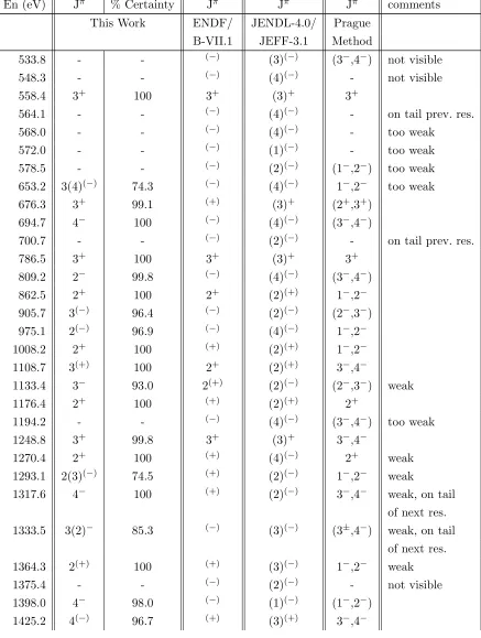
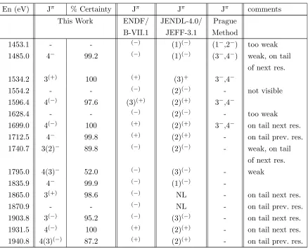
resonances, most resonances with sufficient statistics could be assigned two possible spin values. In Table 4.1, for resonances assigned spin with less than 90% certainty, the second most likely spin value is indicated in parentheses. DANCE data was also analyzed by collaborators using the Prague method. Results using the Prague method are in good agreement with those from this work, and are also shown in Table 4.1.
Table 4.1: Spins, Parities of Neutron Resonances
En (eV) Jπ % Certainty Jπ Jπ Jπ comments
This Work ENDF/ JENDL-4.0/ Prague
/B-VII.1 JEFF-3.1 Method
16.2 1− 99.6 NL (4)− 1−,2−
55.3 3(2)− 79.6 NL (3)− 3−,4−
70.9 2+ 100 2+ (2)+ 2+
79.6 3(−) 94.7 (−) (3)− (2±,3±) on tail prev. res.
109.6 1− 100 (−) (3)− 1−,2−
126.9 - - (−) (4)(−) 2−,3− too weak
136.3 3+ 100 (−) (3)(−) 3−,4−
210.0 2− 100 (−) (3)− 1−,2−
227.6 3+ 99.9 3(−) (3)(+) 3−,4−
233.3 2− 99.6 (−) (1)(−) 1−,2− weak
247.9 3(2)− 82.9 (−) (3)(−) (2−,3−)
268.0 3(+) 100 3+ (3)+ 3+
286.0 2+ 100 2+ (2)+ 2+
312.1 4− 100 3+ (3)+ (3−,4−)
321.1 3(4)− 89.8 (−) (4)(−) (3−,4−)
352.7 4− 100 (−) (2)(−) (3−,4−)
380.9 2+ 100 (−) (4)(−) (1−,2−) on tail next res.
397.2 3(+) 100 3+ (3)+ 3+
457.3 3(2)− 81.8 (−) (3)(−) (3−,4−)
505.5 2+ 100 (−) (3)+ 2+
Table 4.1: Continued
En (eV) Jπ % Certainty Jπ Jπ Jπ comments
This Work ENDF/ JENDL-4.0/ Prague
B-VII.1 JEFF-3.1 Method
533.8 - - (−) (3)(−) (3−,4−) not visible
548.3 - - (−) (4)(−) - not visible
558.4 3+ 100 3+ (3)+ 3+
564.1 - - (−) (4)(−) - on tail prev. res.
568.0 - - (−) (4)(−) - too weak
572.0 - - (−) (1)(−) - too weak
578.5 - - (−) (2)(−) (1−,2−) too weak
653.2 3(4)(−) 74.3 (−) (4)(−) 1−,2− too weak
676.3 3+ 99.1 (+) (3)+ (2+,3+)
694.7 4− 100 (−) (4)(−) (3−,4−)
700.7 - - (−) (2)(−) - on tail prev. res.
786.5 3+ 100 3+ (3)+ 3+
809.2 2− 99.8 (−) (4)(−) (3−,4−)
862.5 2+ 100 2+ (2)(+) 1−,2−
905.7 3(−) 96.4 (−) (2)(−) (2−,3−)
975.1 2(−) 96.9 (−) (4)(−) 1−,2−
1008.2 2+ 100 (+) (2)(+) 1−,2−
1108.7 3(+) 100 2+ (2)(+) 3−,4−
1133.4 3− 93.0 2(+) (2)(−) (2−,3−) weak
1176.4 2+ 100 (+) (2)(+) 2+
1194.2 - - (−) (4)(−) (3−,4−) too weak
1248.8 3+ 99.8 3+ (3)+ 3−,4−
1270.4 2+ 100 (+) (4)(−) 2+ weak
1293.1 2(3)(−) 74.5 (+) (2)(−) 1−,2− weak
1317.6 4− 100 (+) (2)(−) 3−,4− weak, on tail
of next res.
1333.5 3(2)− 85.3 (−) (3)(−) (3±,4−) weak, on tail
of next res.
1364.3 2(+) 100 (+) (3)(−) 1−,2− weak
1375.4 - - (−) (2)(−) - not visible
1398.0 4− 98.0 (−) (1)(−) (1−,2−)
Table 4.1: Continued
En (eV) Jπ % Certainty Jπ Jπ Jπ comments
This Work ENDF/ JENDL-4.0/ Prague
B-VII.1 JEFF-3.1 Method
1453.1 - - (−) (1)(−) (1−,2−) too weak
1485.0 4− 99.2 (−) (1)(−) (3−,4−) weak, on tail
of next res.
1534.2 3(+) 100 (+) (3)+ 3−,4−
1554.2 - - (−) (2)(−) - not visible
1596.4 4(−) 97.6 (3)(+) (2)(+) 3−,4−
1628.4 - - (−) (2)(−) - too weak
1699.0 4(−) 100 (+) (2)(+) 3−,4− on tail next res.
1712.5 4− 99.8 (+) (2)(+) - on tail prev. res.
1740.7 3(2)− 89.8 (−) (2)(−) - weak, on tail
of next res.
1795.0 4(3)− 52.0 (−) (3)(−) - weak
1835.9 4− 99.9 (−) (1)(−)
-1865.0 3(+) 98.6 (−) NL - on tail next res.
1870.9 - - (−) NL - on tail prev. res.
1903.8 3(−) 95.2 (−) (3)(−) - on tail next res.
1931.5 4(−) 100 (+) (2)(+) - on tail next res.
Neutron Energy [eV]
1300 1350 1400 1450 1500
Y
ie
ld
0 500 1000 1500 2000
J=1 J=2 J=3 J=4
Spin Assignment Prototypes
Chapter 5
Neutron Capture Cross-Section and
Resonance Parameters
5.1
Cross Section Calculation
The experimentally measured 97Mo(n,γ) cross section can be expressed as the product of the
components
σn,γ(En) =
M Nn,γ(En)
NAρ f Abeamǫn,γ(En) Φ(En)
, (5.1)
where M is the atomic mass of 97Mo (96.906 u), Nn,γ(En) is the number of capture events
at neutron energy En measured by DANCE, NA is Avogadro’s number (6.022x10²³), Abeam
is the area of the target illuminated by the beam (0.785 cm2), ρ is the areal density of the
molybdenum target (18.7 mg/cm2),ǫn,γ(En) is the total efficiency of DANCE for capturing the
event, and Φ(En) is the neutron flux incident on the target for a given En.
The quantity Nn,γ is measured by the DANCE array, the neutron flux Φ(En) is calculated
using measurements from the neutron beam monitors just downstream from DANCE, and the
efficiencyǫn,γ is calculated using known information.
5.1.1 Neutron Flux
The neutron flux Φ(En) is measured using neutron beam monitors located just past DANCE on
flight path 14. Three neutron monitors are installed: a 6Li silicon detector, a3He proportional
counter, and a 235U fission fragment chamber. Because the last collimator is located upstream
Φ =βΦmon. (5.2)
The absolute neutron flux at the DANCE target must be determined using additional
in-formation. A second target is chosen, one which is geometrically similar to the97Mo target and
isotopically pure, composed of an isotope whose capture cross-section is well determined. The
197Au nucleus fits these criterion well. A target of circular dimensions with a 2.0 cm diameter,
0.1 micron thick layer of gold deposited on a thin strip of mylar was used. The mylar makes a suitable backing material in this case because, as an organic molecule, all of its constituents have total cross sections much smaller than that of gold. DANCE data is collected for the Au target in much the same way as it was collected for the Mo target. The looking time window is shifted to slightly longer times in order to see the large Au resonance at 4.9 eV. The cross section at this resonance is very large (27,000 barns) and is known so precisely that it is often used as a standard for flux determination. Counts from all multiplicities are considered in the capture yield; the counts underneath the resonance are fit with a linear function and subtracted as background. The neutron monitor flux is normalized to this single resonance.
0 5000 10000 15000 20000 25000 30000
4.4 4.6 4.8 5 5.2 5.4 5.6
Cross Section (b)
Neutron Energy [eV]
197Au ENDF Cross Section 197
Au Experiment (normalized)
Figure 5.1: Cross Section of the197Au resonance used to normalize the neutron flux.
Neutron Energy (eV)
10 102 103 104
N e u tr o n F lu x ( n /c m ^ 2 /e V /T o ) -2 10 -1 10 1 10 2 10
Neutron Flux at DANCE
Figure 5.2: Neutron flux measured at DANCE over the duration of the 97Mo experiment.
calculate the effects of beam attenuation and self-shielding by the target. For a target of uniform thickness and composition, that is larger than the beam spot, and is oriented parallel to the incident beam, the beam attenuation is given by a simple formula
Φ(En) = Φo(En)∗e−σtot(En)t, (5.3)
where Φ and Φo are the final and incident beam fluxes, respectively, σtot is the total
cross-section of the target, and t is the target ”thickness” in atoms per barn. For the97Mo nucleus,σtot
is the sum of the capture and elastic cross-sections, and the thickness is 1.162 x10⁻⁴atoms/barn.
The effect of target self-shielding must also be accounted for. As neutrons pass through the target, some fraction are removed from the beam through either capture or scattering reactions. Thus the entire volume of the target is not illuminated with the same flux, resulting in a lower
measured capture yield at the back face of the target than at the front face. For the97Mo target
this reduced yield can be calculated as
Yn,γobs(En) =
Yn,γideal(En) h
1−σn,γ(En)
σtot(En)(1−e
σtot(En)t)
i. (5.4)
experiment.
Neutron Energy [eV]
2
10 103
F ra c ti o n a l E ff e c t -6 10 -5 10 -4 10 -3 10 -2 10 -1 10 1 Mo experiment 97
Effect of Beam Attenuation and Target Self-Shielding for the
Beam Attenuation Target Self-Shielding Beam Attenuation Target Self-Shielding Beam Attenuation Target Self-Shielding
Figure 5.3: Fractional effect of beam attenuation and target self-shielding as a function of neutron energy.
5.1.2 Detection Efficiency of DANCE
The total efficiency of DANCE can be written as the product ofǫo, the efficiency for detecting the
nuclear event andǫgated, the fraction of DANCE events which are included after the application
of multiplicity and summed energy gates
ǫn,γ=ǫoǫgated (5.5)
ǫgated =ǫo
7 X m=3 Ngated Nungated . (5.6)
The modeling of the detector response for DANCE using GEANT4 has been discussed in
great detail in several publications [12], [13]. Sampleγ-ray spectra for simulations were generated
results of DICEBOX for the 97Mo nucleus were used as input for the GEANT4 package. The resulting efficiency of DANCE for detecting a single cascade was 97%, and is comparable to values from other DANCE experiments.
The gated efficiency ǫgated was measured to be 66.0(2)% using counts from the strong
res-onance at 70 eV, where background is low. The total efficiency of DANCE was calculated to be
ǫn,γ = 0.64. (5.7)
5.1.3 Cross Section Results
Utilizing all of the information known concerning the neutron flux, the properties of the target,
and the efficency of DANCE, the neutron capture cross-section for 97Mo was determined to
within 5 percent uncertainty in most regions, and is presented in Figure 5.4. Because the
capture cross-section of 197Au is known very precisely, the 97Mo measurement may still be
called an absolute cross-section.
0.01 0.1 1 10 100 1000
100 1000
Cross Section [b]
Neutron Energy [eV] 97
Mo Experimental Cross Section