ABSTRACT
GAINES, BRIAN RAYMOND. Penalized Estimation in Statistics: Applications & Algorithms. (Under the direction of Eric Chi and Yichao Wu.)
Penalized estimation, also known as regularization, is a modeling framework that has
justifiably received a lot of attention in the statistics and machine learning literature over
the past twenty years. This modeling approach augments a loss function with a penalty
term that can be used to impose structure or prior knowledge on the solution. In this
dissertation, we focus on developing methods for two very different statistical tasks that
both fit into the penalization estimation framework, which highlights the framework’s
flexibility.
For the first method, we compare alternative computing strategies for solving the
constrained lasso problem. As its name suggests, the constrained lasso extends the
widely-used lasso to handle linear constraints, which provide an additional vehicle for
incorporating prior information into the model. In addition to quadratic programming,
we employ the alternating direction method of multipliers (ADMM) and also derive an
efficient solution path algorithm. Through both simulations and real data examples,
we compare the different algorithms and provide practical recommendations in terms of
efficiency and accuracy for various sizes of data. We also show that, for an arbitrary
penalty matrix, the generalized lasso can be transformed to a constrained lasso, while
the converse is not true. Thus, our methods can also be used for estimating a generalized
lasso, which has wide-ranging applications. Code for implementing the algorithms is
freely available in the Matlabtoolbox SparseReg.
The other main method focuses on a different area of statistics, clustering. Clustering
in a dataset. Biclustering extends clustering to two dimensions where both observations
and variables are grouped concurrently, such as simultaneously clustering cancerous
tu-mors and genes or documents and words. Triclustering is then the natural extension of
clustering to three dimensions where the data are organized in a three-dimensional
ar-ray, or tensor. We develop and study a convex formulation of the triclustering problem,
which is guaranteed to obtain a unique global minimum. Convex triclustering generates
an entire solution path of possible triclusters governed by one tuning parameter, and thus
alleviates the need to specify the number of clusters a priori. We extensively study our
©Copyright 2017 by Brian Raymond Gaines
Penalized Estimation in Statistics: Applications & Algorithms
by
Brian Raymond Gaines
A dissertation submitted to the Graduate Faculty of North Carolina State University
in partial fulfillment of the requirements for the Degree of
Doctor of Philosophy
Statistics
Raleigh, North Carolina
2017
APPROVED BY:
Eric Chi
Chair of Advisory Committee
Yichao Wu
Vice-Chair of Advisory Committee
DEDICATION
BIOGRAPHY
The author grew up in the small town of Ossian, Indiana. While Brian was
attend-ing nearby Norwell High School (class of 2002), the rural town had its third stop light
installed, which obviously made the front page of the local newspaper. After high school
Brian first attended college at IPFW, a local satellite campus of Indiana University, for
two years. However, Brian long had his sights set on attending the main Indiana
Uni-versity campus since he, like anyone raised well in Indiana, is a huge fan of the Indiana
Hoosiers. Brian spent three glorious years in Bloomington before graduating in 2007
with a Bachelor of Arts, double majoring in Economics and Political Science.
After college, Brian spent four amazing years working as a research assistant in the
Research Department at the Federal Reserve Bank of Richmond. Brian started working
there shortly before the asset-backed commercial paper market began to dry up, but as we
all know, correlation is not causation. Working as an RA at the Richmond Fed would have
been a great experience even in normal times, but it was especially interesting to be at the
Fed during the financial crisis and Great Recession. While at the Richmond Fed, Brian
also took several math classes at Virginia Commonwealth University to better prepare
himself for the rigors of graduate school. It was during this time that Brian realized his
interest in statistics since, in the words of John Tukey, he likes to “play in everyone’s
backyard.” Brian then spent the next six years studying statistics at North Carolina
State University. Brian was heavily involved in the Department of Statistics, including
a stint as the department’s Graduate Student Association president, the organizer of a
memorable ski trip, and a member of several sports teams, winning three championships.
Shortly after defending his dissertation on 7-27-17, Brian started working at SAS as a
R&D that focuses on increasing the point-and-click capabilities of SAS Studio to make
ACKNOWLEDGEMENTS
I would like to thank my two main advisors, Eric Chi and Hua Zhou, for all of their
guidance, knowledge, and understanding over the last few years. I would also like to
thank Yichao Wu and Donald Martin for serving on my committee. Dr. Zhou effectively
served as my main advisor for two years and as a co-advisor afterwards, but graduate
school policies constrain me from officially recognizing him as such. I am fortunate that
I have been able to continue working with him after he moved to UCLA. I very much
appreciate his emphasis on software development as well as both reproducibility and
professional development. I am also fortunate that Dr. Chi decided to join the NC State
faculty and later serve as my advisor. I actually helped recruit him to NCSU, as I felt
like he would make a nice addition to my committee, and sure enough, I was right. The
fact that he is a relatively young professor is nice because he can relate to what it is like
to be the advisee, and has a lot of “lessons learned” to pass along. Working with him
has definitely made me a more effective researcher.
There are numerous other current and former NC State staff and faculty members I
would like to thank for the knowledge and support they provided me during grad school. I
had the pleasure of teaching under Roger Woodard, Rene´e Moore, Kevin Gross, and Herle
McGowan, all of whom made me a better teacher. I was an instructor for Dr. Woodard
nine different times, so I would like to especially thank him for all of his help and advice,
as well as the help from the Undergraduate Program Assistant, Dana Derosier. I would
also like to acknowledge Dr. Moore, who has continued to be a friend and mentor even
after leaving NC State. Her advice and support were critical to my survival of graduate
school. I am grateful to Emily Griffith and Duncan X. Lascelles for the opportunity to
as the help and advice I received from Justin Post, David Dickey, and Jon Stallings while
in that position. Working as the lead statistician on a variety of projects was invaluable
for my development as a professional statistician. I would like to thank Pam Arroway,
Sujit Ghosh, Howard Bondell, Kim Weems, and Donald Martin for their help and support
while serving as co-directors of the graduate program. I also would like to thank Montse
Fuentes, Leonard Stefanski, and Dennis Boos for their leadership and contributions to
the department. Lastly, I want to thank Alison McCoy for all that she has done for me
and others while serving as a second mom to the graduate students.
The one thing that set NC State apart when I was choosing a graduate program was
the people, and I was not disappointed. As such, and especially given the size of the
program, there are a ton of current and former NCSU graduate students who deserve
recognition, including Todd Regh, Logan Lossing, Dana Lossing, Chad Brown, Kathleen
Brown, Joe Usset, Danny Modlin, Nick Meyer, Neal Grantham, Josh Day, Susheela Singh,
Ali Miller, Marcela Alfaro, So Young Park, Alfredo Farjat, Sarah Hale, Sam Morris, Luke
Smith, Brad Turnbull, Andy Beam, Ander Wilson, David Vock, Brian Naughton, Matt
Austin, Milo Page, and Andrew Wilcox. Todd Regh was my office mate during the first
2-3 years of the program. His advice, humor, and coffee maker helped me survive the first
two years while we logged long hours in the Bureau of Mines. I am also very thankful for
my girlfriend and partner in crime, Colleen McKendry, whose support has kept me afloat
during these final few years of grad school. She also deserves recognition for keeping me
alive when I had a bad case of mononucleosis during my fourth year.
There are several current and former employees of the Richmond Fed that I would like
to acknowledge: Alex Wolman, Roy Webb, Kartik Athreya, Jeff Lacker, Ned Prescott,
Arantxa Jarque, John Walter, Ray Owens, Bob Hetzel, Tanya Hockaday, Rita Franklin,
Sarah Watt, Mark House, Jake Blackwood, Devin Reilly, Sabrina Pellerin, Sonya Waddell,
Nick Haltom, and Renee Haltom. My arrival at the Richmond Fed could not have been
timed any better, not only in terms of being there during the financial crisis but also in
terms of the employees I overlapped with, many of whom are still good friends. I would
like to especially thank Alex Wolman for taking a chance and giving me the unbelievable
opportunity to work at the Fed. I am also especially grateful for Sabrina Pellerin, who
is like a long-lost fraternal twin, and among other things was instrumental in helping me
realize that NC State was the right place for me. She also helped renew my interest in
tennis, a hobby that has been crucial in helping an admitted workaholic take breaks from
school and maintain my sanity. It has also been a joy to watch her two awesome kids,
Holden and Alyana, grow up.
Last and most importantly, I truly believe that I would not be here without my
unbelievably amazing family and friends, whom I am immensely and eternally grateful
for. Above all, I would like to thank my parents, Allen and Susan Gaines, for all they
have done for me over the years. How they raised me has given me such a huge leg
up in life, and for that I will forever be grateful. Over the years I have been fortunate
to have been integrated into several families, which has meant the world to me: the
Wilsons, DBs, Deckers, Eckerts, and Wyatts. I would like to especially thank Clark and
Monica Eckert, Cody Griner, Caleb Decker, Bill Decker, Mark McAfee, Travis White,
and Brad Grear. As clich´e as it sounds, they are like brothers and sisters to me. I also
would like to thank Adam and Kylie McCartney, Keith Koch, Tom Koch, Tracy Koch,
David Stead, Josh Gerber, Dustin Weikel, Greg Bunn, Phil McAfee, John Feeney, Connie
and Wouter Bolte, Monica and Scott Van Arsdale, Brandie Dafforn, and Jamie Costello.
Clark, Monica, Cody, and David were intricate in making IU some of the best years of
Harper, and it has been really great to watch their kids grow up. More broadly, Monica’s
entire family deserves special recognition for the support they have provided me during
several family vacations and holidays, which was crucial for maintaining sanity during
grad school. Terri and George Eckert, as well as Bill and Karen Decker, have been second
(and third) parents to me. Caleb, Mark, Travis, and Brad have provided endless good
times and laughs over the years. I also would like to thank my Little League baseball
coach, Mark De La Garza, for instilling in me a strong work ethic that I have relied on
heavily to get to this point. Lastly, I would like to thank Paul Oakenfold, Sound Tribe
Sector 9, Michael Franti, Tool, Three 6 Mafia, Lil Wayne, and the Notorious B.I.G. for
TABLE OF CONTENTS
LIST OF TABLES . . . xi
LIST OF FIGURES . . . xii
Chapter 1 Introduction . . . 1
1.1 Penalized Estimation . . . 1
Chapter 2 Algorithms for Fitting the Constrained Lasso . . . 6
2.1 Introduction . . . 6
2.2 Connection to the Generalized Lasso . . . 10
2.3 Algorithms . . . 15
2.3.1 Quadratic Programming . . . 16
2.3.2 ADMM . . . 17
2.3.3 Path Algorithm . . . 19
2.4 Simulated Examples . . . 25
2.4.1 Sum-to-zero Constraints . . . 26
2.4.2 Non-negativity Constraints . . . 29
2.5 Real Data Applications . . . 31
2.5.1 Global Warming Data . . . 31
2.5.2 Brain Tumor Data . . . 32
2.5.3 Microbiome Data . . . 34
2.6 Conclusion . . . 37
Chapter 3 Generalized Convex Clustering. . . 39
3.1 Introduction . . . 39
3.2 Generalized Convex Clustering . . . 43
3.2.1 Motivation . . . 43
3.2.2 Formulation . . . 44
3.2.3 Results . . . 46
3.3 Discussion . . . 46
Chapter 4 Convex Triclustering . . . 48
4.1 Introduction . . . 48
4.2 Preliminaries: Tensor Background and Notation . . . 50
4.2.1 Tensor Basics . . . 50
4.2.2 Tensor Operations . . . 53
4.2.3 Tensor Decompositions . . . 55
4.3 Literature Review . . . 58
4.3.2 Multi-way Clustering . . . 62
4.3.3 Clustering Tensor Objects . . . 63
4.4 A Convex Formulation of Triclustering . . . 66
4.4.1 Formulation . . . 66
4.4.2 Properties . . . 69
4.4.3 Estimation . . . 70
4.5 Practical Considerations . . . 78
4.5.1 Specifying the Weights . . . 78
4.5.2 Choosing ρ . . . 80
4.6 Simulation Studies . . . 82
4.6.1 Cubical Tensors, Checkerbox Pattern . . . 85
4.6.2 Rectangular Tensors . . . 93
4.6.3 CANDECOMP/PARAFAC Model . . . 99
4.6.4 Importance of Good Weights . . . 101
4.7 Real Data Application . . . 103
4.8 Discussion . . . 108
References . . . 110
Appendices . . . 131
Appendix A Additional Constrained Lasso Derivations . . . 132
A.1 Constrained Lasso via Generalized Lasso . . . 132
A.1.1 Reparameterization . . . 132
A.1.2 Null-Space Method . . . 134
A.2 Subgradient Violations . . . 136
Appendix B Additional Convex Triclustering Simulation Results . . . 140
B.1 Checkerbox Pattern: Balanced Sizes and Homoskedasticity . . . 141
B.2 Checkerbox Pattern: Imbalanced Sizes and Homoskedasticity . . . . 147
B.3 Checkerbox Pattern: Balanced Sizes and Heteroskedasticity . . . 151
B.4 Different Clustering Structures . . . 155
B.5 Rectangular Tensors . . . 157
B.6 CP Model, Adjusted Rand Index . . . 163
LIST OF TABLES
Table 2.1 Solution Path Events . . . 22
LIST OF FIGURES
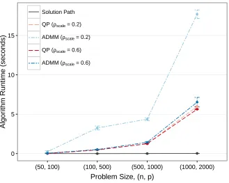
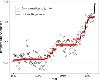
Figure 2.1 Global Warming Data. Annual temperature anomalies relative to the 1961-1990 average. . . 8 Figure 2.2 Simulation 1 Results: Algorithm Runtime. Average algorithm runtime
(seconds) plus/minus one standard error for a constrained lasso with sum-to-zero constraints on the coefficients. The solution path’s runtime is av-eraged across the number of kinks in the path to make the runtime more comparable to the other algorithms estimated at one value of the tuning parameter, ρ=ρscale·ρmax. . . 27
Figure 2.3 Simulation 1 Results: Algorithm Accuracy. Objective value error (per-cent) relative to quadratic programing (QP) for the solution path and ADMM at different values of ρscale =ρ/ρmax for (n, p) = (500,1000). The results are qualitatively the same for the other combinations of (n, p) con-sidered. . . 28 Figure 2.4 Simulation 2 Results: Algorithm Runtime. Average algorithm runtime
(seconds) plus/minus one standard error for a constrained lasso with non-negativity constraints on the parameters. The solution path’s runtime is averaged across the number of kinks in the path to make the runtime more comparable to the other algorithms which are estimated at one value of the tuning parameter, ρ=ρscale·ρmax. . . 30 Figure 2.5 Global Warming Data. Annual temperature anomalies relative to the
1961-1990 average, with trend estimates using isotonic regression and the constrained lasso. . . 32 Figure 2.6 Brain Tumor Data. Sparse fused lasso estimates on the brain tumor data
using both the generalized lasso and the constrained lasso. . . 35 Figure 2.7 Microbiome Data Solution Paths. Comparison of solution path coefficient
estimates on the microbiome dataset using both (a) zero-sum regression and (b) the constrained lasso. . . 37
Figure 4.1 Fibers of a Third-order Tensor. Source: Kolda & Bader (2009). . . 52 Figure 4.2 Slices of a Third-order Tensor. Source: Kolda & Bader (2009). . . 52 Figure 4.3 Rank-one Third-order Tensor. X =a◦b◦c, where the (i, j, k) element
is xijk =aibjck. Source: Kolda & Bader (2009). . . 55
Figure 4.4 CP Decomposition. The CP decomposition (4.7) of a third-order tensor. Source: Kolda & Bader (2009). . . 57 Figure 4.5 Tucker Decomposition. The Tucker decomposition (4.9) of a third-order
tensor. Source: Kolda & Bader (2009). . . 58 Figure 4.6 Tensor with Checkerbox Structure. Each mode has two clusters for a
Figure 4.7 Example Weights-Induced Edge Graph. A graph with positive weights for ωm,12, ωm,15, and ωm,34 and zero weights between all other nodes, cor-responding to the mode-m slices. Source: Chi & Lange (2015). . . 67 Figure 4.8 Checkerbox Simulation Results: Impact of Noise Level. Two balanced
clusters per mode across different levels of homoskedastic noise for I1 = I2 =I3 = 60. Average triclustering performance plus/minus one standard error. . . 87 Figure 4.9 Checkerbox Simulation Results: Impact of Cluster Size Imbalance.
Two imbalanced clusters per mode with either low or high homoskedastic noise for I1 =I2=I3 = 60. Average triclustering performance plus/minus one standard error for different degrees of cluster size imbalance. Low noise corresponds to σ = 3 (SNR = 13) while high noise refers to σ = 6 (SNR =
1
6). Size ratio = 0.5 corresponds to balanced clusters. . . 89
Figure 4.10 Checkerbox Simulation Results: Impact of Heteroskedasticity. Two balanced clusters per mode with either low or high heteroskedastic noise for I1 = I2 =I3 = 60. Average triclustering performance plus/minus one standard error for different levels of heteroskedasticity. Low noise corre-sponds to σ = 3 (SNR = 13) while high noise refers to σ = 6 (SNR = 16). Noise ratio = 1 corresponds to homoskedastic noise. . . 91 Figure 4.11 Checkerbox Simulation Results: Impact of Clustering Structure.
Dif-ferent number of balanced clusters per mode with either low or high ho-moskedastic noise for I1 = I2 = I3 = 60. Average triclustering perfor-mance plus/minus one standard error for different clustering structures, corresponding to either three clusters per mode or two, three, and four clusters along modes one, two, and three. Low noise corresponds to σ = 3 (SNR = 13) while high noise refers toσ= 6 (SNR = 16). . . 92 Figure 4.12 Checkerbox Simulation Results: Impact of Tensor Shape. Two
bal-anced clusters per mode with two levels of homoskedastic noise for a tensor with two short modes and one longer mode. Average adjusted rand index plus/minus one standard error for different noise levels and mode lengths. 95 Figure 4.13 Checkerbox Simulation Results: Impact of Tensor Shape. Two
bal-anced clusters per mode with two levels of homoskedastic noise for a tensor with one short modes and two longer modes. Average adjusted rand index plus/minus one standard error for different noise levels and mode lengths. 96 Figure 4.14 Checkerbox Simulation Results: Impact of Tensor Shape. Two
Figure 4.16 CP Model Simulation Results. Two balanced clusters per mode with low homoskedastic noise for I1 = I2 = I3 = 40. Average triclustering performance plus/minus one standard error for two different data generation approaches. “Bullseye” and “Half Moons” refer to the shape embedded in the factor matrices used to generate the true tensor (Figure 4.15). . . 101 Figure 4.17 Impact of Convex Triclustering Weights. Comparison of different weights
for convex triclustering for clustering a cubical tensor with two balanced clusters per mode and homoskedastic noise withI1=I2=I3= 60. Average triclustering performance plus/minus one standard error for different noise levels. TD1 refers to using a Tucker decomposition with the rank chosen using the SCORE algorithm (Section 4.5.1. Trueuses the true mean tensor
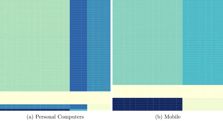
U to construct the weights, while Datauses the noisy data tensor X. . . 102 Figure 4.18 Advertisement and Publisher Click-Through Rate Biclusters for a
Ran-dom User. Advertisements are on the y-axis and publishers are on the x-axis. Darker blue corresponds to higher click-through rates for a given device. . . 108
Figure B.1 Checkerbox Simulation Results: Impact of Noise Level. Two balanced clusters per mode across different levels of homoskedastic noise for I1 = I2=I3= 40. Average adjusted rand index plus/minus one standard error. 141 Figure B.2 Checkerbox Simulation Results: Impact of Noise Level. Two balanced
clusters per mode across different levels of homoskedastic noise for I1 = I2 = I3 = 40. Average variation of information plus/minus one standard error. . . 142 Figure B.3 Checkerbox Simulation Results: Impact of Noise Level. Two balanced
clusters per mode across different levels of homoskedastic noise for I1 = I2=I3= 60. Average adjusted rand index plus/minus one standard error. 143
Figure B.4 Checkerbox Simulation Results: Impact of Noise Level. Two balanced clusters per mode across different levels of homoskedastic noise for I1 = I2 = I3 = 60. Average variation of information plus/minus one standard error. . . 144 Figure B.5 Checkerbox Simulation Results: Impact of Noise Level. Two balanced
clusters per mode across different levels of homoskedastic noise for I1 = I2=I3= 80. Average adjusted rand index plus/minus one standard error. 145 Figure B.6 Checkerbox Simulation Results: Impact of Noise Level. Two balanced
clusters per mode across different levels of homoskedastic noise for
Figure B.7 Checkerbox Simulation Results: Impact of Cluster Size Imbalance with Low Noise. Two imbalanced clusters per mode with low (σ = 3, SNR =
1
3) homoskedastic noise and I1 = I2 = I3 = 60. Average adjusted rand
index plus/minus one standard error for different degrees of cluster size imbalance. Size ratio = 0.5 corresponds to balanced clusters. . . 147 Figure B.8 Checkerbox Simulation Results: Impact of Cluster Size Imbalance with
Low Noise. Two imbalanced clusters per mode with low (σ = 3, SNR = 1
3) homoskedastic noise and I1 = I2 = I3 = 60. Average variation of information plus/minus one standard error for different degrees of cluster size imbalance. Size ratio = 0.5 corresponds to balanced clusters. . . 148 Figure B.9 Checkerbox Simulation Results: Impact of Cluster Size Imbalance with
High Noise. Two imbalanced clusters per mode with high (σ = 6, SNR = 16) homoskedastic noise and I1 = I2 =I3 = 60. Average adjusted rand index plus/minus one standard error for different degrees of cluster size imbalance. Size ratio = 0.5 corresponds to balanced clusters. . . 149 Figure B.10 Checkerbox Simulation Results: Impact of Cluster Size Imbalance with
High Noise. Two imbalanced clusters per mode with high (σ = 6, SNR = 16) homoskedastic noise and I1 = I2 = I3 = 60. Average variation of information plus/minus one standard error for different degrees of cluster size imbalance. Size ratio = 0.5 corresponds to balanced clusters. . . 150 Figure B.11 Checkerbox Simulation Results: Impact of Heteroskedasticity with
Low Noise. Two balanced clusters per mode with low (σ = 3, SNR = 1
3) heteroskedastic noise and I1=I2 =I3= 60. Average adjusted rand in-dex plus/minus one standard error for different levels of heteroskedasticity. Noise ratio = 1 corresponds to homoskedastic noise. . . 151 Figure B.12 Checkerbox Simulation Results: Impact of Heteroskedasticity with
Low Noise. Two balanced clusters per mode with low (σ = 3, SNR = 13) heteroskedastic noise and I1 =I2 =I3 = 60. Average variation of informa-tion plus/minus one standard error for different levels of heteroskedasticity. Noise ratio = 1 corresponds to homoskedastic noise. . . 152 Figure B.13 Checkerbox Simulation Results: Impact of Heteroskedasticity with
High Noise. Two balanced clusters per mode with high (σ = 6, SNR = 16) heteroskedastic noise and I1 =I2 =I3 = 60. Average adjusted rand index plus/minus one standard error for different levels of heteroskedastic-ity. Noise ratio = 1 corresponds to homoskedastic noise. . . 153 Figure B.14 Checkerbox Simulation Results: Impact of Heteroskedasticity with
Figure B.15 Checkerbox Simulation Results: Impact of Clustering Structure. Dif-ferent number of balanced clusters per mode with either low or high ho-moskedastic noise for I1 = I2 = I3 = 60. Average triclustering perfor-mance plus/minus one standard error for different clustering structures, corresponding to either three clusters per mode or two, three, and four clusters along modes one, two, and three. Low noise corresponds to σ = 3 (SNR = 13) while high noise refers toσ= 6 (SNR = 16). . . 155 Figure B.16 Checkerbox Simulation Results: Impact of Clustering Structure.
Dif-ferent number of balanced clusters per mode with either low or high ho-moskedastic noise for I1 = I2 = I3 = 60. Average variation of informa-tion plus/minus one standard error for different clustering structures, cor-responding to either three clusters per mode or two, three, and four clusters along modes one, two, and three. Low noise corresponds to σ= 3 (SNR =
1
3) while high noise refers to σ= 6 (SNR = 1
6). . . 156
Figure B.17 Checkerbox Simulation Results: Impact of Tensor Shape. Two bal-anced clusters per mode with two levels of homoskedastic noise for a tensor with two short modes and one longer mode. Average adjusted rand index plus/minus one standard error for different noise levels and mode lengths. 157 Figure B.18 Checkerbox Simulation Results: Impact of Tensor Shape. Two
bal-anced clusters per mode with two levels of homoskedastic noise for a tensor with two short modes and one longer mode. Average variation of infor-mation plus/minus one standard error for different noise levels and mode lengths.. . . 158 Figure B.19 Checkerbox Simulation Results: Impact of Tensor Shape. Two
bal-anced clusters per mode with two levels of homoskedastic noise for a tensor with one short mode and two longer modes. Average adjusted rand index plus/minus one standard error for different noise levels and mode lengths. 159 Figure B.20 Checkerbox Simulation Results: Impact of Tensor Shape. Two
bal-anced clusters per mode with two levels of homoskedastic noise for a tensor with one short mode and two longer modes. Average variation of infor-mation plus/minus one standard error for different noise levels and mode lengths. . . 160 Figure B.21 Checkerbox Simulation Results: Impact of Tensor Shape. Two
Figure B.22 Checkerbox Simulation Results: Impact of Tensor Shape. Two bal-anced clusters per mode with two levels of homoskedastic noise for a tensor with short, medium, and long mode lengths. Average variation of infor-mation plus/minus one standard error for different noise levels and mode lengths. . . 162 Figure B.23 CP Model Simulation Results. Two balanced clusters per mode with low
homoskedastic noise for I1 = I2 = I3 = 40. Average adjusted rand index plus/minus one standard error for two different data generation approaches. “Bullseye” and “Half Moons” refer to the shape embedded in the factor matrices used to generate the true tensor (Figure 4.15). . . 163 Figure B.24 CP Model Simulation Results. Two balanced clusters per mode with low
Chapter 1
Introduction
Variable selection and prediction are two fundamental goals in statistics and
ma-chine learning. Penalization, also referred to as regularization or shrinkage, is a flexible
framework that can be used to achieve either task. In this dissertation, we focus on two
methods that are used for very different statistical tasks but both fit into the penalized
estimation framework. This highlights the framework’s flexibility. In this chapter, we
first motivate penalization in the context of regression before discussing the general
pe-nalized estimation framework. For a more-detailed treatment of the subject, see Hastie
et al. (2009).
1.1
Penalized Estimation
Consider the standard linear regression model,
for i = 1, ..., n, where yi is the response or outcome variable for the ith observation,
xi ∈ Rp is a vector of predictor or feature variables (covariates) for the ith observation
whose jth element is xij, β ∈ Rp is the vector of unknown regression coefficients to
be estimated, and εi is an independently and identically distributed error term. Using
matrix notation, we can equivalently write the model (1.1) as
y=Xβ+ε, (1.2)
where
y=
y1
y2
.. .
yn
X =
x11 x12 · · · x1p
x21 x22 · · · x2p
..
. ... · · · ...
xn1 xn2 · · · xnp
ε=
ε1
ε2
.. .
εn
,
and β =
β1, β2, . . . , βp
T
. The typical approach to estimating the parameter vector β
is to perform ordinary least squares (OLS) by solving the minimization problem
ˆ
β = arg min
β
n
X
i=1
(yi − p
X
j=1
xijβj)2 (1.3)
= arg min
β
ky−Xβk2 2.
Assuming that the data (design) matrixX has full column rank, then (1.3) has the
well-known solution ˆβ = (XTX)−1XTy. Despite its wide use and elegant theory, the linear regression model has its shortcomings. Its prediction accuracy can often be improved
upon, it does not automatically perform variable selection, and its solution is not unique
One way to improve upon the linear model is to augment it with a penalty term,
ρJ(β), so the objective function becomes
ˆ
β(ρ) = arg min
β
ky−Xβk2
2+ρJ(β)
, (1.4)
where ρ ≥ 0 is the penalization parameter, also called the tuning or regularization
pa-rameter, and J(β) is a user-specified penalty function. Although it is common in the
statistical literature to denote the penalty parameter by λ, we instead use ρ since it
is common in constrained optimization to use λ to represent the Lagrange multipliers
(dual variables). The penalization parameter, ρ, controls the bias-variance trade-off by
governing how much weight is put on the penalty function when solving (1.4) for the
coefficient estimates. When ρ= 0, the penalty term drops out and the estimates match
the OLS estimates, but asρincreases, more emphasis is put on the penalty function. To
understand the role played by the penalty function J(β), consider using the`1 norm for
the penalty, so J(β) = kβk1 =
Pp
j=1|βj|. With this penalty function, the optimization
problem becomes
ˆ
β(ρ) = arg min
β
ky−Xβk22+ρkβk1
. (1.5)
The model (1.5) is known as the lasso, which stands for the Least Absolute Shrinkage
and Selection Operator and was proposed by Tibshirani (1996) in a seminal work. The
lasso (1.5) can equivalently be formulated as a constrained regression problem,
minimize
β ky−Xβk
2
2 (1.6)
where there is a one-to-one correspondence betweentandρfrom (1.5) (Tibshirani, 1996).
The constrained formulation (1.6) makes the role of the penalty function more clear,
as we can see that the constraint shrinks the magnitudes of the estimated regression
coefficients as t decreases. One benefit of using the `1 norm for the penalty is that,
due to the geometry of the absolute value function (a sharp kink at zero), the `1 norm
shrinks some coefficients to be exactly zero and thus simultaneously performs continuous
variable selection and estimation at the same time (Hastie et al., 2009). For this reason,
it is typically recommended to standardize the data matrixX in penalized regression to
put the predictors on the same scale so the penalization is done equitably.
More generally, given a data matrix X, the goal is to estimate a function f(X) to
model or predict the response of interest, y. The general penalization framework for
doing so is given by
minimize
f∈H
n X
i=1
L(yi, f(xi)) +ρJ(f)
, (1.7)
where L(yi, f(xi)) is a loss function, f is a function belonging to some space of
func-tions H, ρ ≥ 0 is a penalization parameter, and J(f) is a penalty functional (Hastie
et al., 2009). The loss function measures how well the estimated values fit the
ob-served values. The most commonly used loss function is the squared error loss function,
L(yi, f(xi)) = (yi −f(xi))2, which is used for OLS regression (1.3). Other loss
func-tions include absolute error, a negative log-likelihood for generalized linear models, and
the hinge loss for support vector machines (Hastie et al., 2009). One way to view the
penalty function is that it allows the user to incorporate prior knowledge or structure
into the estimation. For example, in the case of the lasso (1.5), the prior knowledge is
(Hastie et al., 2009). The lasso essentially spawned a new area of research devoted to
tweaking the penalization framework (1.7), typically by modifying the penalty term. As
such, several popular methods in statistics can fit into this framework, including ridge
regression (Hoerl & Kennard, 1970), the lasso (Tibshirani, 1996), adaptive lasso (Zou,
2006), group lasso (Yuan & Lin, 2006), graphical lasso (Yuan & Lin, 2007; Friedman
et al., 2008), generalized lasso (Tibshirani & Taylor, 2011), fused lasso (Tibshirani et al.,
2005), `1 trend filtering (Kim et al., 2009), elastic net (Zou & Hastie, 2005), smoothing
splines (O’Sullivan, 1986), convex clustering (Lindsten et al., 2011; Hocking et al., 2011),
Chapter 2
Algorithms for Fitting the
Constrained Lasso
2.1
Introduction
Our focus is on estimating the constrained lasso problem (James et al., 2013)
minimize 1
2ky−Xβk
2
2+ρkβk1 (2.1)
subject to Aβ =b and Cβ≤d,
where y ∈ Rn is the response vector, X ∈
Rn×p is the data matrix of predictors or covariates, β∈Rp is the vector of unknown regression coefficients, and ρ≥0 is a tuning
parameter that controls the amount of penalization. It is assumed that the constraint
matrices, AandC, both have full row rank. As its name suggests, the constrained lasso
augments the standard lasso (1.5) with linear equality and inequality constraints. While
estimates in terms of sparsity, the constraints provide an additional vehicle for prior
knowledge to be incorporated into the solution. For example, consider the annual data on
temperature anomalies given in Figure 2.1. As has been previously noted in the literature
on isotonic regression, temperature generally appears to increase monotonically over the
time period of 1850 to 2015 (Wu et al., 2001; Tibshirani et al., 2011). This monotonicity
can be imposed on the coefficient estimates using the constrained lasso with the inequality
constraint matrix
C=
1 −1
1 −1 . .. ...
1 −1
andd=0∈Rp−1. The lasso with a monotonic ordering of the coefficients was referred to
by Tibshirani & Suo (2016) as theordered lasso, and is a special case of the constrained
lasso (2.1).
Another example of the constrained lasso that has appeared in the literature is the
positive lasso. First mentioned in the seminal work of Efron et al. (2004), the positive
lasso requires the lasso coefficients to be non-negative. This variant of the lasso has seen
applications in areas such as vaccine design (Hu et al., 2015b), nuclear material detection
(Kump et al., 2012), document classification (El-Arini et al., 2013), and portfolio
manage-ment (Wu et al., 2014). The positive lasso is a special case of the constrained lasso (2.1)
withC =−Ip andd=0p. Additionally, there are several other examples throughout the
literature where the original lasso is augmented with additional information in the form
of linear equality or inequality constraints. Huang et al. (2013b) constrained the lasso
−0.4 0.0 0.4 0.8
1850 1900 1950 2000
Year
T
emper
ature Anomalies
Figure 2.1: Global Warming Data. Annual temperature anomalies relative to the 1961-1990 average.
with the presence of a certain protein in a cell or tissue. The lasso with a sum-to-zero
constraint on the coefficients has been used for regression (Shi et al., 2016) and variable
selection (Lin et al., 2014) with compositional data as covariates. Compositional data
are multivariate data that represent proportions of a whole and thus must sum to one,
and are seen in applications such as consumer spending in economics, topic consumption
of documents in machine learning, and the human microbiome (Lin et al., 2014). Lastly,
simplex constraints were utilized by Huang et al. (2013a) when using the lasso to estimate
edge weights in brain networks. Thus, the constrained lasso is a very flexible framework
for imposing additional knowledge and structure onto the lasso coefficient estimates.
He (2011) that also derived a solution path algorithm for solving the constrained lasso.
However, our approach to deriving the path algorithm is completely different and is more
in line with the literature on solution path algorithms (Rosset & Zhu, 2007), especially in
the presence of constraints (Zhou & Lange, 2013). Additionally, we address how our
al-gorithms can be adapted to work in the high-dimensional setting wheren < p, which was
not done by He (2011). Furthermore, the approach by He (2011) decomposes the
param-eter vector,β, into its positive and negative parts,β =β+−β−, thus doubling the size of the problem. On the other hand, we work directly with the original coefficient vector at
the benefit of computational efficiency and notational simplicity. Another important
con-tribution of our work is the implementation of our algorithms in theSparseRegMatlab
toolbox available on Github.
The constrained lasso was also studied by James et al. (2013) in an earlier version of
their manuscript on penalized and constrained (PAC) regression. The current PAC
re-gression framework extends (2.1) by using a negative log likelihood for the loss function to
also cover generalized linear models (GLMs), and thus is more general than the problem
we study. However, the increased generality of their method comes at the cost of
compu-tational efficiency. Furthermore, their path algorithm is not a traditional solution path
algorithm as it is fit on a pre-specified grid of tuning parameters, which is fundamentally
different from our path following strategy. Additionally, we believe the squared error loss
function merits additional attention given its widespread use with the `1 penalty, and
also since the constrained lasso is a natural approach to solving constrained least squares
problems in the increasingly common high-dimensional setting. Hu et al. (2015a) studied
the constrained generalized lasso, which reduces to the constrained lasso when no penalty
matrix is included (D=Ip). However, they do not derive a solution path algorithm but
The rest of the chapter is organized as follows. In Section 2.2, we demonstrate a new
connection between the constrained lasso and the generalized lasso, which shows that the
latter can always be transformed and solved as a constrained lasso, even when the penalty
matrix is rank deficient. Given the flexibility of the generalized lasso, this result greatly
extends the applicability of our algorithms and results. Various algorithms to solve
the constrained lasso, including quadratic programming (QP), the alternating direction
method of multipliers (ADMM), and a novel path following algorithm, are derived in
Section 2.3. Simulation results that compare the performance of the various algorithms
are presented in Section 2.4. The main result from the simulations is that, in terms of
runtime the solution path algorithm is more efficient than the other approaches when
the coefficient estimates are desired at more than a handful of values of the penalization
parameter. Real data examples that highlight the flexibility of the constrained lasso are
given in Section 2.5, while Section 2.6 concludes.
2.2
Connection to the Generalized Lasso
Another flexible lasso formulation is the generalized lasso (Tibshirani & Taylor, 2011)
minimize 1
2ky−Xβk
2
2+ρkDβk1, (2.2)
where D ∈ Rm×p is a fixed, user-specified regularization matrix. Certain choices of D
correspond to different versions of the lasso, including the original lasso, various forms of
the fused lasso, and trend filtering. It has been observed that (2.2) can be transformed
to a standard lasso when D has full row rank (Tibshirani & Taylor, 2011), and it can
be transformed to a constrained lasso whenD has full column rank (James et al., 2013).
lasso (2.1) for an arbitrary penalty matrix D.
Assume that rank(D) = r, and consider the singular value decomposition (SVD)
D=UΣVT =
U1,U2
Σ1 0
0 0
VT
1
V2T
=U1Σ1V
T
1 ,
where U1 ∈Rm×r, U2 ∈Rm×(m−r), Σ1 ∈Rr×r, V1 ∈Rp×r, and V2 ∈Rp×(p−r). We define
an augmented matrix
˜ D=
U1Σ1V1T
VT
2
=
U1Σ1 0
0 Ip−r
VT
1
VT
2
=
U1Σ1 0
0 Ip−r
V
T
and use the following change of variables
α
γ
= ˜Dβ =
U1Σ1V1T
V2T
β, (2.3)
where α ∈ Rm and γ ∈
Rp−r. Since the matrix V2T forms a basis for the nullspace of
D, N(D), it has rank p−r and its columns are linearly independent of the columns of
D. Thus, the augmented matrix ˜D has full column rank, and the new variables
α
γ
uniquely determine β via
β = ( ˜DTD˜)−1D˜T
α γ = V
Σ1U1T 0
0 Ip−r
U1Σ1 0
0 Ip−r
V T −1 ˜ DT α γ = V
Σ1U1TU1Σ1 0
0 Ip−r
V T −1 ˜ DT α γ = V
Σ21 0
0 Ip−r
V T −1 ˜ DT α γ = (V
T)−1
Σ21 0
0 Ip−r
−1
V−1
˜ DT α γ = V
Σ−12 0
0 Ip−r
V T ˜ DT α γ = V
Σ−12 0
0 Ip−r
V TV
Σ1U1T 0
0 Ip−r
α γ = V
Σ−12 0
0 Ip−r
Σ1U1T 0
0 Ip−r
α γ = V
Σ−12Σ1U1T 0
0 Ip−r
α γ =
V1 V2
Σ−11U1T 0
0 Ip−r
α γ
where D+ denotes the Moore-Penrose inverse of the matrix D. However, since the
original change of variables is
α
γ
= ˜Dβ, β is uniquely determined if and only if
α
γ
∈ C( ˜D) =C
U1Σ1 0
0 Ip−r
,
if and only if
α∈ C(U1Σ1) =C(U1) =C(D),
if and only if
U2Tα=0m−r,
where C(D) is the column space of the matrix D. Therefore, the generalized lasso
problem (2.2) is equivalent to a constrained lasso problem
minimize α,γ
1 2
y−XD+α−XV2γ
2
2+ρkαk1 (2.4)
subject to U2Tα=0m−r,
where γ remains unpenalized. There are three special cases of interest:
1. When D has full row rank, r = m, the matrix U2 is null and the constraint
U2Tα = 0m−r vanishes, reducing to a standard lasso as observed by Tibshirani &
Taylor (2011).
drops, resulting in a constrained lasso as observed by James et al. (2013).
3. When D does not have full rank, r < min(m, p), the above problem (2.4) can be
simplified to a constrained lasso problem only in α by noticing that minimizing
(2.4) with respect toγ yields
XV2γˆ = PXV2(y−XD +α)
for anyα, wherePXV2 is the orthogonal projection onto the column spaceC(XV2).
Thus, for an arbitrary penalty matrix D, using the change of variables (2.3) we
end up with a constrained lasso problem
minimize 1
2ky˜−Xα˜ k
2
2+ρkαk1
subject to U2Tα=0m−r,
where ˜y = (I−PXV2)y and ˜X = (I−PXV2)XD
+. The solution path ˆα(ρ) can
be translated back to that of the original generalized lasso problem via the affine
transform
ˆ
β(ρ) = V1Σ−11U
T
1 αˆ(ρ) +V2(V2TX
TXV
2)−V2TX
T[y−XD+αˆ(ρ)]
= [I−V2(V2TX
T
XV2)−V2TX
T
X]D+αˆ(ρ)
+V2(V2TX
TXV
2)−V2TX
Ty,
where X− denotes the generalized inverse of a matrix X.
Thus, any generalized lasso problem can be reformulated as a constrained lasso, so the
it is not always possible to transform a constrained lasso into a generalized lasso, as
detailed in Appendix A.1.
2.3
Algorithms
In this section, we derive three different algorithms for estimating the constrained
lasso (2.1). Throughout this section, we assume that X has full column rank, which
necessitates that n > p. For the increasingly prevalent high-dimensional case where
n < p, we follow the standard approach in the related literature (Tibshirani & Taylor,
2011; Hu et al., 2015a; Arnold & Tibshirani, 2016) and add a small ridge penalty to the
original objective function in (2.1). The problem then becomes
minimize 1
2ky−Xβk
2
2+ρkβk1+
ε
2kβk
2
2 (2.5)
subject to Aβ =b and Cβ≤d,
where ε is some small constant, such as 10−4. Note that the objective (2.5) can be re-arranged into standard constrained lasso form (2.1)
minimize 1 2ky
∗ −
(X∗)βk2
2+ρkβk1 (2.6)
subject to Aβ =b and Cβ≤d,
using the augmented data y∗ =
y
0
andX
∗ =
X √
εIp
. The augmented data matrix
has full column rank, so the following algorithms can then be applied to the augmented
form (2.6). As discussed by Tibshirani & Taylor (2011), this approach is attractive for
improve predictive accuracy.
Before deriving the algorithms, we first define some notation. For a vectorvand index
setS, let vS be the sub-vector of size |S| containing the elements of v corresponding to
the indices in S, where | · | denotes the cardinality or size of the index set. Similarly,
for a matrix M and another index set T, the matrix MST contains the rows from M
corresponding to the indices inS and the columns ofM from the indices inT. We use a
colon, :, when all indices along one of the dimensions are included. That is,MS:contains
the rows from M corresponding to S but all of the columns in M.
2.3.1
Quadratic Programming
Our first approach is to use quadratic programming to solve the constrained lasso
problem (2.1). The key is to decompose β into its positive and negative parts, β =
β+ −β−, as the relation |β| = β+ +β− handles the `1 penalty term. By plugging
these into (2.1) and adding the additional non-negativity constraints on β+ and β−, the constrained lasso is formulated as a standard quadratic program of 2p variables,
minimize 1 2
β+
β−
T
XTX −XTX
−XTX XTX
β+
β−
+
ρ12p−
XTy
−XTy
T
β+
β−
subject to
A −A
β+
β−
=b
C −C
β+
β−
≤d
β+≥0p, β
Matlab’s quadprog function is able to scale up to p ∼ 102-103, while the commercial
Gurobi Optimizer is able to scale up to p∼103-104.
2.3.2
ADMM
The next algorithm we apply to the constrained lasso problem (2.1) is the
alternat-ing direction method of multipliers (ADMM). The ADMM algorithm has experienced
renewed interest in statistics and machine learning applications in recent years as it can
solve a large class of problems, is often easy to implement, and is amenable to distributed
computing; see Boyd et al. (2011) for a recent survey. In general ADMM is an algorithm
to solve a problem that features a separable objective but coupling constraints,
minimize f(x) +g(z)
subject to M x+F z =c,
where f, g : Rp 7→
R∪ {∞} are closed proper convex functions. The idea is to employ block coordinate descent to the augmented Lagrangian function followed by an update
of the dual variables ν,
x(t+1) ← arg min
x
Lτ(x,z(t),ν(t))
z(t+1) ← arg min
z
Lτ(x(t+1),z,ν(t))
ν(t+1) ← ν(t)+τ(M x(t+1)+F z(t+1)−c),
where t is the iteration counter and the augmented Lagrangian is
Lτ(x,z,ν) = f(x) +g(z) +νT(M x+F z−c) + τ
2kM x+F z−ck
2
Often it is more convenient to work with the equivalent scaled form of ADMM, which
scales the dual variable and combines the linear and quadratic terms in the augmented
Lagrangian (2.7). The updates become
x(t+1) ← arg min
x
f(x) + τ
2kM x+F z
(t)−
c+u(t)k22
z(t+1) ← arg min
z
g(z) + τ 2kM x
(t+1)
+F z−c+u(t)k22
u(t+1) ← u(t)+M x(t+1)+F z(t+1)−c,
where u = ν/τ is the scaled dual variable. The scaled form is especially useful in the
case where M =F =I, as the updates can be rewritten as
x(t+1) ← proxτ f(z(t)−c+u(t))
z(t+1) ← proxτ g(x(t+1)−c+u(t))
u(t+1) ← u(t)+x(t+1)+z(t+1)−c,
where proxτ f is the proximal mapping of a function f with parameter τ > 0. Recall
that the proximal mapping is defined as
proxτ f(v) = argmin
x
f(x) + 1
2τkx−vk
2 2
.
One benefit of using the scaled form for ADMM is that, in many situations including the
constrained lasso, the proximal mappings have simple, closed form solutions, resulting in
straightforward ADMM updates. To apply ADMM to the constrained lasso, we identify
1 Initialize β(0) =z(0) =β0, u(0) =0p,τ > 0 ;
2 repeat
3 β(t+1) ←argmin12ky−Xβk22+21τkβ+z(t)+u(t)k22+ρkβk1; 4 z(t+1)←projC(β(t+1)+u(t));
5 u(t+1) ←u(t)+β(t+1)+z(t+1);
6 until convergence criterion is met;
Algorithm 1: ADMM for solving the constrained lasso (2.1).
Rp :Aβ =b,Cβ≤d},
g(β) = δC(β) =
∞ β∈ C/
0 β∈ C.
For the updates, proxτ f is a regular lasso problem and proxτ g is a projection onto the
affine spaceC (Algorithm 1). The projection onto convex sets is well-studied and, in many
applications, can be solved analytically (see Section 15.2 of Lange (2013) for several
examples). For situations where an explicit projection operator is not available, the
projection can be found by using quadratic programming to solve the dual problem,
which has a smaller number of variables.
2.3.3
Path Algorithm
In this section we derive a novel solution path algorithm for the constrained lasso
problem (2.1). According to the KKT conditions, the optimal pointβ(ρ) is characterized
by the stationarity condition
coupled with the linear constraints. Here s(ρ) is the subgradient∂kβk1 with elements
sj(ρ) =
1 βj(ρ)>0
[−1,1] βj(ρ) = 0
−1 βj(ρ)<0
, (2.8)
and µ satisfies the complementary slackness condition. That is, µl = 0 if cTl β < dl and
µl≥0 if cTl β=dl.
Along the path we need to keep track of two sets,
A := {j :βj 6= 0}, ZI := {l:cTl β =dl}.
The first set indexes the non-zero (active) coefficients and the second keeps track of the set
of (binding) inequality constraints on the boundary. Focusing on the active coefficients
for the time being, we have the (sub)vector equation
0|A| = −X:TA(y−X:AβA) +ρsA+AT:Aλ+CZTIAµZI (2.9)
b
dZI
=
A:A CZIA
βA,
involving dependent unknownsβA,λ, andµZI, and independent variableρ. Applying the implicit function theorem to the vector equation (2.9) yields the path following direction
d dρ
βA λ
µZI
=−
XT
:AX:A AT:A CZTIA A:A 0 0 CZIA 0 0
−1
sA
0
0
The right hand side is constant on a path segment as long as the sets A and ZI and the
signs of the active coefficients sA remain unchanged. This shows that the solution path of the constrained lasso is piecewise linear. The involved matrix is non-singular as long
asX:A has full column rank and the constraint matrix
A:A CZIA
has linearly independent
rows. The stationarity condition restricted to the inactive coefficients
−X:TAc[y−X:AβA(ρ)] +ρsAc(ρ) +AT:Acλ(ρ) +CZT
IAcµZI(ρ) = 0|Ac|
determines
ρsAc(ρ) =X:TAc[y−X:AβA(ρ)]−AT:Acλ(ρ)−CZT
IAcµZI(ρ). (2.11)
ThusρsAc moves linearly along the path via
d
dρ[ρsAc] =−
X:TAX:Ac A:Ac CZIAc
T
d dρ
βA λ
µZI
. (2.12)
The inequality residual rZc
I :=CZIcAβA−dZIc also moves linearly with gradient
d
dρrZcI =CZ c IA
d
dρβA. (2.13)
Together, equations (2.10), (2.12), and (2.13) are used to monitor changes to A and ZI,
which can potentially result in kinks in the solution path.
To recap, since the solution path is piecewise linear we only need to monitor the events
be interpolated. A summary of these events is given in the left-hand side of Table 2.1.
We perform path following in the decreasing direction fromρmax towardsρ= 0. Letβ(t)
denote the solution at kink t, then the next kink t+ 1 is identified by the smallest ∆ρ,
where ∆ρ > 0 is determined by the conditions listed in the right column of Table 2.1.
In addition to monitoring these events along the path, we also need to ensure that the
Table 2.1: Solution Path Events
Event Monitor
An active coefficient hits 0 β(At)−∆ρdρdβ(At) =0|A|
An inactive coefficient becomes active [ρ(t)s(At)c]−∆ρdρd[ρsAc] =±(ρ(t)−∆ρ)1|Ac|
A strict inequality constraint hits the boundary rZ(t)c I −∆ρ
d
dρrZIc =0|ZIc|
An inequality constraint escapes the boundary µ(Zt)
I −∆ρ
d
dρµZI =0|ZI|
subgradient conditions (2.8) remain satisfied. An issue arises when inactive coefficients
on the boundary of the subgradient interval are moving too slowly along the path such
that their subgradient would escape [-1, 1] at the next kink t+ 1. To handle this issue,
if an inactive coefficient βj, j ∈ Ac, with subgradient sj = ±1 is moving too slowly,
the coefficient is moved to the active set A and equation (2.10) is recalculated before
continuing the path algorithm. See Appendix A.2 for the explicit ranges of dρd[ρsAc] that need to be monitored and the corresponding derivations.
Initialization
Since we perform path following in the decreasing direction, a starting value for the
is given by
minimize kβk1 (2.14)
subject to Aβ =b and Cβ≤d,
which is a standard linear programming problem. We first solve (2.14) to obtain initial
coefficient estimates β0 and the corresponding sets A and ZI, as well as initial values
for the Lagrange multipliers λ0 and µ0. Following Rosset & Zhu (2007), path following
begins from
ρmax= max
xTj(y−Xβ0)−AT:jλ0−CZT
Ijµ
0
ZI
, (2.15)
and the subgradient is set according to (2.8) and (2.11). As noted by James et al.
(2013), this approach can fail when (2.14) does not have a unique solution. For example,
consider a constrained lasso with a sum-to-one constraint on the coefficients, P
jβj = 1.
Any elementary vector ej, which has a 1 for the jth element and 0 otherwise, satisfies
this constraint while also achieving the minimum`1 norm, resulting in multiple solutions
to (2.14). In this case, it is still possible to use (2.14) and (2.15) to identify ρmax, which
is then used in (2.1) to initialize β0, A, ZI, λ0, and µ0 via quadratic programming.
Termination
Another practical consideration for implementing the solution path algorithm is a
principled approach to terminating the algorithm. To this end, we derive a formula for
the degrees of freedom of the constrained lasso. The standard approach in the lasso
on the expression for degrees of freedom given by Stein (1981),
df(g) = E
" n X
i=1
∂gi ∂yi
#
, (2.16)
where g is a continuous and almost differentiable function, which with g(y) = ˆy =Xβˆ
is satisfied in our case (Hu et al., 2015a). In order to apply (2.16), we need to assume
that the response is normally distributed,
y∼N(µ, σ2In).
As before, we also assume that both constraint matrices, A and C, have full row rank,
and X has full column rank. Then, using the results in Hu et al. (2015a) withD =Ip,
for a fixed ρ≥0 the degrees of freedom are given by
df(Xβˆ(ρ)) = E [|A| −(q+|ZI|)], (2.17)
where |A| is the number of active predictors, q is the number of equality constraints,
and |ZI| is the number of binding inequality constraints. The unbiased estimator for
the degrees of freedom is then |A| −(q +|ZI|). This result is intuitive as the degrees
of freedom start out as the number of active predictors, and then one degree of freedom
is lost for each equality constraint and each binding inequality constraint. Additionally,
when there are no constraints, (2.1) becomes a standard lasso problem with degrees of
freedom equal to |A|, consistent with the result in Zou et al. (2007). The formula (2.17)
is also consistent with results for constrained estimation presented in Zhou & Lange
solution path algorithm, as the path terminates once the degrees of freedom equaln. The
number of degrees of freedom is also an important measure that is an input for several
metrics used for model assessment and selection, such as Mallows’Cp(Mallows, 1973), the
Akaike information criterion (AIC) (Akaike, 1974), or the Bayesian information criterion
(BIC) (Schwarz et al., 1978). Specifically, these criteria can be plotted along the path
as a function of ρ as a technique for selecting the optimal value for the penalization
parameter, as alternatives to cross-validation.
2.4
Simulated Examples
To investigate the performance of the various algorithms outlined in Section 2.3 for
solving a constrained lasso problem, we consider two simulated examples. For both
simulations, we used the three different algorithms discussed in Section 2.3 to solve (2.1).
As noted in Section 2.3.2, the ADMM algorithm includes an additional tuning parameter
τ, which we fix at 1/n based on initial experiments. Additionally, as pointed out in Boyd
et al. (2011), the performance of the ADMM method can be greatly impacted by the
choice of the algorithm’s stopping criteria, which we set to be 10−4 for both the absolute and relative error tolerances. We also used a user-defined function handle to solve the
subproblem of projecting onto the constraint set for ADMM as this improves efficiency.
Two factors of interest in the simulations are the size of the problem, (n, p), and the value
of the penalization tuning parameter,ρ. Four different levels were used for the size factor,
(n, p): (50, 100), (100, 500), (500, 1000), and (1000, 2000). For the latter factor, the
values ofρwere calculated as a fraction of the maximumρ. The fractions, or ρscale values
(i.e., ρ = ρscale ·ρmax) used in the simulations were 0.2, 0.4, 0.6, and 0.8, to investigate
how the degree of penalization impacts algorithm performance. Since the runtimes for
solution path algorithm is averaged across the number of kinks in the path to make the
results more comparable. To generate the data for both simulations, the covariates in
the data matrix, X, were generated as independent and identical (iid) standard normal
variables, and the response was generated as y = Xβ +ε where ε ∼ N(0n,In). Both
simulations used 20 replicates and were conducted in Matlab using the SparseReg toolbox on a computer with an Intel i7-6700 3.4 GHz processor and 32 GB memory.
Quadratic programming uses the Gurobi Optimizer via the Matlab interface, while
ADMM and the path algorithm are pure Matlab implementations.
2.4.1
Sum-to-zero Constraints
The first simulation involves a sum-to-zero constraint on the true parameter vector,
P
jβj = 0. Recently, this type of constraint on the lasso has seen increased interest as
it has been used in the analysis of compositional data as well as analyses involving any
biological measurement analyzed relative to a reference point (Lin et al., 2014; Shi et al.,
2016; Altenbuchinger et al., 2016). Written in the constrained lasso formulation (2.1),
this corresponds to A =1Tp and b = 0. For this simulation, the true parameter vector,
β, was defined such that the first 25% of the entries are 1, the next 25% of the entries are
-1, and the rest of the elements are 0. Thus the true parameter satisfies the sum-to-zero
constraint, which we can impose on the estimation using the constraints.
The main results of the simulation are given in Figure 2.2, which plots the average
al-gorithm runtime results across different problem sizes, (n, p). The results using quadratic
programing (QP) and ADMM are each graphed at two values ofρscale, 0.2 and 0.6. In the
graph we can see that the solution path algorithm was faster than the other methods,
and its relative performance is even more impressive as the problem size grows. The