©
DOI: 10.1534/genetics.104.035410
A Model Selection-Based Interval-Mapping Method for Autopolyploids
Dachuang Cao,* Bruce A. Craig* and R. W. Doerge*
,†,1*Department of Statistics, Purdue University, West Lafayette, Indiana 47907 and†Department of Agronomy, Purdue University, West Lafayette, Indiana 47907
Manuscript received August 24, 2004 Accepted for publication January 14, 2005
ABSTRACT
While extensive progress has been made in quantitative trait locus (QTL) mapping for diploid species, similar progress in QTL mapping for polyploids has been limited due to the complex genetic architecture of polyploids. To date, QTL mapping in polyploids has focused mainly on tetraploids with dominant and/or codominant markers. Here, we extend this view to include any even ploidy level under a dominant marker system. Our approach first selects the most likely chromosomal marker configurations using a Bayesian selection criterion and then fits an interval-mapping model to each candidate. Profiles of the likelihood-ratio test statistic and the maximum-likelihood estimates (MLEs) of parameters including QTL effects are obtained via the EM algorithm. Putative QTL are then detected using a resampling-based significance threshold, and the corresponding parental configuration is identified to be the underlying parental configuration from which the data are observed. Although presented via pseudo-doubled back-cross experiments, this approach can be readily extended to other breeding systems. Our method is ap-plied to single-dose restriction fragment autotetraploid alfalfa data, and the performance is investigated through simulation studies.
Q
UANTITATIVE trait loci (QTL) mapping detects polyploidrepresents species with homology in betweenand identifies the regions of a genome associated allopolyploids and autopolyploids (Suzukiet al.1989). with the variation of a quantitative trait of interest. Mo- For allopolyploids (or disomic polyploids), such as bread lecular markers have been used extensively to construct wheat and potato, meiosis is usually restricted to the genetic maps for diploid species (Koornneefet al.1983; pairing of ancestral parental homologs. Thus, the
genet-Dietrichet al.1996) and act as the foundation for QTL ics of allopolyploids are similar to those of diploids, and
analyses such as interval mapping (Lander and Bot- diploid QTL-mapping methods can be carried out by
stein1989;Knappet al.1990;HaleyandKnott1992), treating each of the two sets of homologous chromo-composite interval mapping (Zeng1993, 1994), and mul- somes from an ancestral genome as a diploid.
tiple-QTL mapping (Jansen1993). The statistical issues in- For autopolyploids (or polysomic polyploids), however, volved in diploid QTL mapping are reviewed inDoerge the high ploidy level and homology create
complica-et al.(1997),Broman(2001), andDoerge(2002). tions in interpreting the meiotic process. Unlike
dip-Polyploids are organisms having more than two com- loids whose two homologs always pair during meiosis, plete sets of chromosomes in a cell. Polyploidy is most autopolyploids may undergo either bivalent pairing common in plants, but also found in some insects, am- (two chromosomes pair) or multivalent pairing (more
phibians, and reptiles. Some 30–70% of today’s angio- than two chromosomes pair) (Muller1916;Newton
sperms and at least half of the flowering plants are and Darlington 1929; Darlington 1931; Sybenga
thought to be polyploid (SoltisandSoltis1999). Not 1995). Furthermore, the manner in which the paired only is polyploidy important in agriculture, but it is also chromosomes segregate during meiosis, especially for an important evolutionary force (Soltis and Soltis multivalent pairing, varies in different species (Mather
2000;Wolfe2001;Osbornet al.2003;Soltiset al.2003). 1938; RiesebergandDoyle 1989;Jacksonand Jack-To describe the current state of QTL mapping in poly- son1996). Finally, the marker genotypes in autopoly-ploids, they must first be classified according to their ho- ploids are not always identifiable (i.e., the banding mology. A polyploid with genomes all derived from the patterns are not unique since not all the alleles can be same species is called an autopolyploid. If the multiple differentiated by any one marker system). Even if we are sets of chromosomes are derived from different species, able to identify the different alleles of one locus, the the polyploid is called anallopolyploid. Asegmental
allo-number of copies (dosage) of each allele and the link-age phases (i.e., the arrangement of alleles on the infor-mative chromosomes) between loci remain unknown. 1Corresponding author:Department of Statistics, Purdue University,
There are two different approaches for dealing with
1399 Math Bldg., West Lafayette, IN 47907.
E-mail: [email protected] the multiple copies of one locus for autopolyploids.
With a dominant marker system, each locus is treated tal marker dosages, parental QTL configuration, and QTL effect. Initially, we estimate the parental marker as biallelic. For this case,Wuet al. (1992) estimated a
genetic map for autopolyploids with simplex markers, or dosages using progeny marker data to reduce the num-ber of potential parental configurations. On the basis single-dose restriction fragment (SDRF) markers, which
represent only one homolog and segregate 1:1 in the of each putative parental configuration, interval map-ping is performed to estimate QTL location and to cal-progeny. Ripol et al. (1999) extended the method of
Wuet al.(1992) to any dominant marker with an unob- culate maximum-likelihood estimates of QTL effect and
population variation that are obtained using the expec-servable dosage level. With codominant markers each
locus is treated as multiallelic (Luo et al. 2000, 2001; tation maximization (EM) algorithm (Dempster et al.
1977). We limit our approach to any even ploidy level
Hackett et al.2001). Each band observed on a gel is
viewed as a different allele for that locus. This approach with multiple-dose dominant markers since odd ploidy levels are often associated with high infertility. After is valid for some marker systems, such as simple sequence
repeats (SSRs) that do not require the use of DNA describing the methodology, our method is applied to
single-dose restriction fragment alfalfa data with an esti-digestion by restriction enzymes and whose motifs have
high variation in the number of repeat units. However, mated linkage map fromBrouwerandOsborn(1999). Several putative QTL have been identified as associated since the use of SSRs may be responsible for inaccurate
allele identification,RodzenandMay(2002) suggested with winter hardiness traits in bivalent tetraploid alfalfa and act as the basis of simulation studies that investigate scoring multiallelic SSR markers as individual dominant
markers, unless the markers’ underlying modes of in- the performance of our approach.
heritance are known, simply because different loci may have different inheritance patterns. Because the
avail-METHODS
ability of codominant markers for autopolyploids is
rela-tively rare, and dominant markers (e.g., SDRF markers) Our polyploid QTL-mapping methodology is devel-oped for organisms undergoing bivalent pairing during have the advantages of being rich in plants and easily
scored, the remainder of this article is based on the meiosis. Under the bivalent pairing assumption, the pairing of the chromosomes can range frompreferential
dominant marker system.
An additional advantage of using SDRF markers is that pairing(always pairing with the same homologous chro-mosome) torandom pairing(equally likely to pair with the only unknown factor is the linkage phase (coupling
or repulsion) between the SDRFs and this can be esti- any other homologous chromosome). The data analysis and simulation are based on random pairing.
mated by a goodness-of-fit test. In turn, the
maximum-likelihood estimate (MLE) of the recombination between Letndenote the number of progeny andkdenote the ploidy level. In what follows, for each locus, uppercase is SDRF markers can be calculated on the basis of the
estimated linkage phase. Using SDRFs, Brouwer and used to denote both the locus name and its dominant
allele, and lowercase represents the recessive allele (e.g.,
Osborn (1999) estimated the first composite genetic
map for tetraploid alfalfa. When considering multiple- M1andm1). The dosage of a locus refers to the number of copies of the dominant allele at that locus. For exam-dose markers,Ripolet al. (1999) first estimated marker
dosages and linkage phase and then constructed the ple, a locus dosage of two refers to two copies of the dominant allele at that locus. When a marker is ob-genetic map by computing the maximum-likelihood
estimate of recombination fraction on the basis of esti- served,at leastone copy of the dominant allele for that marker is present.
mated parental marker configurations.DoergeandCraig
(2000) extended polyploid QTL methodology by devel- Marker data (presence/absence) and the quantitative
trait data are measured on the F1progeny. These prog-oping an algorithmic model selection process for a
sin-gle-marker QTL analysis with dominant markers for eny are the result of a pseudo-doubled backcross
ex-periment (Figure 1), where an informative parent P1is autopolyploids with any even ploidy level. Recently,Luo
et al.(2004) addressed both bivalent and quadrivalent crossed with a noninformative parent P2. The dosage at
each locus in the parents is at least one for the informa-chromosomal pairing during meiosis by employing a
sta-tistical framework for the analysis of tetrasomic linkage. tive parent and zero for the noninformative parent. Furthermore, at most half of the chromosomes of the As a continuation of the work byDoergeandCraig
(2000), we propose an interval-mapping method by em- informative parent contain dominant alleles. Chromo-somes that contain dominant alleles in the informative ploying an available genetic map to increase the power
of detecting and estimating QTL locations within an parent are called informative chromosomes. The pseudo-doubled backcross design is equivalent to doubling the autopolyploid bivalent pairing framework. For
simplic-ity, and in keeping with this previous work, we base our half of the noninformative chromosomes of the infor-mative parent to produce the noninforinfor-mative parent work on a pseudo-doubled backcross experiment (
Grat-tapagliaandSederoff1994) and employ a model selec- and then crossing them to get F1. An example of a pseudo-doubled backcross experiment for a tetraploid (k⫽4) tion-based interval mapping to simultaneously estimate
Figure 2.—Possible parental marker configurations for a tetraploid with two marker loci (M1/m1andM2/m2) under a pseudo-doubled backcross design. (A) Double coupling. (B) Asymmetric coupling 12. (C) Asymmetric coupling 21. (D) Coupling. (E) Repulsion.
Figure1.—A pseudo-doubled backcross experiment for a all the dosages of QTL. The vector ⫽ ( ⫽ (0, 1, tetraploid with two loci. Each locus is assumed to be biallelic:
. . . ,k/2), ) is used to denote model parameters. At
M1/m1andM2/m2, whereM1andm1denote two alleles of the
any fixed putative position of the QTL the likelihood
first locus andM1is the dominant allele, and similarly forM2
andm2. For each locus, there are two copies of the dominant function of the trait is a mixture of normal distributions allele in the informative parent P1. P2is the noninformative (Equation 1) under the assumption of one QTL, doubled haploid produced by doubling a haploid of P1, which
contains only recessive alleles.
L(|x,c)⫽
兿
ni⫽1
兺
k/2j⫽0
P(dQ⫽ j|Ii,c)φ(yi;j,2)
䉭
⫽
兿
ni⫽1
兺
k/2j⫽0
j|iφ(yi;j,2), (1) In this case, the dosage for both markers is two in the
informative parent. A pseudo-doubled backcross
popu-lation can also be developed from diploids by choosing whereP(d
Q⫽j|Ii,c) ⫽ 䉭 j|iis the probability of theith two homozygous parents carrying different alleles,
dou-bling each of them to produce tetraploids, crossing progeny having dosageence statusI jof the QTL given marker pres-i, andφ(yi;j,2) denotes the normal den-them to produce an F1, and then crossing the F1to the sity function valued aty
iwith meanjand variance2.
parent containing recessive alleles. Thej
|i’s are a function of parental configurationc and
Interval mapping:Consider two flanking markers,M1 the recombination fractions between the QTL and
andM2, and one QTL,Q, with marker genetic distance markers.
or recombination fraction provided by an available ge- In the interval-mapping framework (Lander and
netic map. Once the parental configurationcis known, Botstein1989), the putative QTL is considered at in-interval mapping can be applied to locate QTL. A paren- cremental positions in an interval defined by adjacent tal configuration includes loci dosages and linkage markers, and a test statistic (commonly the log-likeli-phase. If the dominant alleles of two loci are on the hood ratio) is evaluated. LetR
h(h ⫽1, 2) denote the
same chromosome, they are in coupling phase; other- true recombination fractions between markerM
h and wise, they are in repulsion phase. On the basis of this, QTL. At each evaluation position, letr
h(h⫽1, 2) denote the five respective configurations for a tetraploid with the recombination fractions between markers defining
two markers under a pseudo-doubled backcross design the interval and the current QTL position. The
log-are called double coupling (Figure 2A), asymmetric cou- likelihood-ratio test statistic is calculated to test the hy-pling 12 (Figure 2B), asymmetric couhy-pling 21 (Figure 2C), pothesis
coupling (Figure 2D), and repulsion (Figure 2E).
Simi-H0: Rh⫽0.5,h ⫽1, 2 larly, there are three possible QTL configurations: (1)
one dose of the QTL located on the first informative H
a: Rh⫽rh,h⫽1, 2. chromosome, (2) one dose of the QTL on the second
The null hypothesis assumes that the QTL is present, informative chromosome, and (3) two doses of the QTL
but unlinked to both markers, while the alternative hy-on both informative chromosomes. In what follows, chy-on-
con-pothesis assumes that the QTL is present and linked to figurations A–E are used to denote a marker
configura-M1 and M2 with recombination fractions rh. The log-tion for a tetraploid as defined above. A marker
config-likelihood-ratio test statistic LRT is uration letter followed by a QTL configuration number
represents acompleteparental configuration, such as “A1,”
LRT⫽ ⫺2 ln L(ˆ0,R1⫽R2⫽0.5)
L(ˆa,R1⫽r1,R2⫽r2) , which represents a parental configuration with markers
in double coupling and one QTL on the first
informa-tive chromosome. whereˆ0andˆaare MLEs under the null and alternative
For theith individual, the observed data arexi⫽(yi, hypotheses, respectively. If the test statistic is significant
Ii), where yi is the trait value, and Ii is the indicator then the corresponding interval position with the largest vector for marker presence (i.e.,Iih⫽1 if markerMhis LRT statistic is considered as the estimated QTL posi-present and 0 otherwise). Assume for each QTL dosage tion. A permutation test can be performed to estimate levelj(j⫽0, 1, . . . ,k/2) that the traityhas a normal the significance threshold for the test statistic (
Because the summation format of the likelihood func- form the candidate parental configuration set. The joint method, on the other hand, takes a similar approach, tion (1) causes difficulty in finding the MLE of, the
complete likelihood function, containing both observ- but information on all markers is considered jointly. In this case, parental marker configuration posterior able and unobservable data, is considered,
probabilities are calculated directly, and candidate
pa-L(|x)⫽
兿
n
i⫽1
兿
k/2j⫽0
[j|iφ(yi;j,2)]zi j, (2) rental configurations are chosen using the same posterior probability rule as described for the marginal method. and the EM algorithm (Dempsteret al.1977) is employed Given the marginal marker presence/absence distri-to estimate. Here, the unobservable data {zi⫽(zi0, . . . , bution (Ripolet al.1999), the posterior probabilities for
zi,k/2)}ni⫽1, wherezij⫽1 if the QTL dosage for theith prog- parental marker dosages of each marker are calculated eny isjand 0 otherwise, are indicator vectors represent- using Bayes’ rule (Bayes1783). For one markerM, the
ing progeny QTL dosages. number of progeny withMabsent,n⭋, has a binomial
dis-To implement the EM algorithm, the E step and M tribution Bin(n,pdM), wheredMdenotes the marker dos-step are iterated until a convergence criterion of the age ofMin the informative parent. Under the pseudo-log-likelihood (e.g., logLt⫹1⫺logLt⬍10⫺6) is satisfied. double backcross design,
In the E step, the missing datazi jare estimated on the
basis of the observable data, and, in the M step, the p
dM⫽
冢
k⫺dM
k/2
冣
冒
冢
k k/2
冣
MLE ofare calculated using the estimatedzij. Aftertiterations, estimated values ofzi jt,t, andtare used at
for random pairing. Thus, given the informative parent stept⫹1 such that thezijt⫹1are estimated in the E step by
marker dosagedM,
zt⫹1
ij ⫽P(dQ⫽j|xi,c,t,t)
P(N⭋⫽n⭋|n,dM) ⫽䉭 Bin(n⭋;n,dM)⫽
冢
n n⭋冣
pn⭋
dM(1⫺pdM)
n⫺n⭋. ⫽ j|iexp{⫺1⁄2((yi ⫺ tj)/t)2}
兺
k/2l⫽0l|iexp{⫺1⁄2((yi⫺ tl)/t)2} .
Let denote the prior distribution of marker dosage Givenzijt⫹1, the MLE of⫽(,) is obtained (M step) dM. The posterior probability of each dosage level is by maximizing (2),
P(dM|n,n⭋)⫽
Bin(n⭋;n,pdM)(dM)
兺
k/2d⫽1Bin(n⭋;n,pd)(d) t⫹1
j ⫽
兺
n i⫽1ztij⫹1yi兺
ni⫽1ztij⫹1
, j⫽0, 1, . . . ,k/2;
⫽ p n⭋
dM(1⫺pdM)n⫺n⭋(dM)
兺
k/2 d⫽1pn⭋
d(1⫺pd)n⫺n⭋(d) . t⫹1 ⫽
冪
1n
兺
n
i⫽1
兺
k/2j⫽0
zt⫹1
ij (yi⫺ tj⫹1)2.
As an alternative method to the described marginal ap-proach, we use the joint marker information and genetic map to calculate the posterior probability of a parental Since the estimation procedure is based on a specific
parental configuration (model), the model space
ex-pands quickly as the marker number and/or ploidy marker configuration. Given markers M
1 and M2, all level increase. Enumerating each possible model for the progeny can be classified into four sets according to the purpose of exploring which is most likely to produce presence status of the two markers. Letn
obs⫽(n00,n01,
the observed data and then estimating parameters on n
10, n11) denote the observed frequency vector in the the basis of the most likely model(s) is computationally four sets, where the hth (h ⫽1, 2) subscript is 1 ifM
h challenging. For example, under a pseudo-doubled back- is present and 0 otherwise. Assuming no segregation cross design with two markers and one QTL, there are distortion and a parental configurationc, the distribu-14 possible parental configurations for a tetraploid, 91 tion ofn
obsfollows a multinomial distribution with proba-for a hexaploid (k⫽6), and 390 for an octaploid (k⫽ bility parameter vector pc⫽(pc
00,pc01,pc10,pc11). Table 1 8). To reduce these computations, we employ a model lists pc for a tetraploid. The probability of observing
reduction step prior to parameter estimation. n
obs⫽(n00,n01,n10,n11) is
Model reduction: To reduce the model space, one
can consider one of two approaches: either a marginal P(n
obs|n,c) ⫽䉭 Multinomial(nobs;n,c)⫽
n!
兿
1i,j⫽0nij!
兿
1i,j⫽0 {pc
ij}ni j. or a joint statistical method. Under the marginal method,
we calculate the posterior probability of dosages for
each marker individually. If one particular dosage level Letdenote the prior distribution of marker configu-has a posterior probability higher than a specified cut- ration c 僆 C. The posterior probability for a specific off, only that marker dosage is considered in candidate parental marker configurationc
0僆Cis parental configurations. Otherwise, we select the most
likely dosage levels until the sum of posterior probabili- P(c
0|n,nobs)⫽
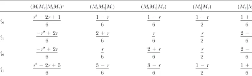
TABLE 1 Multinomial distribution probability parameterspc⫽(pc
00,pc01,pc10,pc11) in a tetraploid with
two markers under random pairing
(M1M2|M1M2)a (M1M2|M1) (M1M2|M2) (M1|M2) (M2|M1)
p00c
r2⫺2r⫹1 6
1⫺r 6
1⫺r 6
1⫺r 2
1⫹r 6
p01c
⫺r2⫹2r 6
2⫹r 6
r 6
r 2
2⫺r 6
p10c
⫺r2⫹2r 6
r 6
2⫹r 6
r 2
2⫺r 6
p11c
r2⫺2r⫹5 6
3⫺r 6
3⫺r 6
1⫺r 2
1⫹r 6
r, estimated recombination fraction between the two markers.
aOnly dominant alleles are shown for informative chromosomes, separated by |.
correct marker dosages for both marker loci, while for the joint method it refers to selecting the correct marker ⫽
兿
1
i,j⫽0{pcij0}ni j(c0)
兺
c僆C兿
1i,j⫽0{pijc}ni j(c).
configuration. The proportion of data sets for which a unique configuration was selected,puni, was also recorded Among the many criteria for assessing the worth of
as a measurement of the efficiency for reducing the model a model reduction method are ease of implementation,
space (Table 3). In general, both methods performed a high probability of selecting the correct model, and
better with a larger sample size and shorter marker efficiency in reducing the size of the candidate model
distances. With sample sizeⱖ100, bothpincandpuniwere
space. Even though the marginal method is easy to im- ⵑ
1.0 for all the simulation settings. With a small sample plement and less computationally expensive, the joint
size, the extra information from the genetic map added method directly estimates the posterior probability of
strength to the joint method both in selecting the cor-parental marker configurations. One might expect that
rect configuration and in reducing the model space. because there may be multiple marker configurations that
On the basis of the simulation results, the joint model have the same marker dosages, especially if the marker
reduction method is recommended for data analysis. dosages are low and ploidy high, the joint method will
Once the model reduction step is completed, the be more efficient in reducing the model space.
selected submodels are used to form the pool of candi-A simulation study was performed to compare the
date parental marker configurations by combining these performance of the marginal and joint methods for a
submodels with possible parental QTL configurations. tetraploid under random pairing. We chose two markers
After this, the likelihood function is constructed for each and marker genetic distance varied from 0.1 to 0.5 M
candidate parental configuration, and the EM algorithm with 0.1-M increments. Sample sizes ranged from 50 to
is applied to maximize the likelihood function and esti-500 with increments of 50. For each simulation setting,
mate parameters. The parental configuration that has 10,000 data sets were generated. The cutoff probability
the maximal likelihood is then identified as the parental was set to be 0.90 for both methods. Without any prior
configuration from which the observed data have arisen. information concerning the parental marker
configura-tion, we assumed all the possible parental marker config-urations to be equally likely (i.e., the prior for the joint
DATA ANALYSIS
method is discrete uniform). Under this assumption, the
The proposed approach was employed to analyze a prior distribution of a marker dosage is not uniform since
published alfalfa SDRF data set with traits related to a lower dosage is more frequent than a higher dosage.
winter hardiness (BrouwerandOsborn1999). Alfalfa Among the five possible parental marker configurations
is an autotetraploid that undergoes bivalent random (Figure 2, A–E) for a tetraploid, dosage 1 has a frequency of
pairing (BinghamandMcCoy1988;Caoet al.2004). 3/5 and dosage 2 has a frequency of 2/5 for each marker
Winter hardiness is a complex trait and one of the most locus. In turn, this frequency distribution was used as the
important adaptations for alfalfa. Because there is no prior of marker dosage for the marginal method.
direct measurement of winter hardiness, related traits The proportion of data sets for which the correct
con-including winter injury (WI), fall growth (FG), freezing figuration was included in the candidate configuration
injury (FI), and unifoliate internode length (UIL) were space, pinc, was recorded (Table 2) for both methods.
TABLE 2
Estimatedpinc, probability of selecting the correct configuration in the candidate configuration (model)
space, for a tetraploid with two markers, 10,000 simulated data sets, and a cutoff of 0.90 for both the marginal and joint model reduction methods under random pairing
n
50 100 150
0.1a 0.3 0.5 0.1 0.3 0.5 0.1 0.3 0.5
Marginal
(M1M2|M1M2) 1.000 1.000 1.000 1.000 1.000 1.000 1.000 1.000 1.000 (M1M2|m1M2) 0.992 0.992 0.991 0.999 0.999 0.999 1.000 1.000 0.999 (M1M2|M1m2) 0.992 0.992 0.993 0.999 0.999 0.999 1.000 0.999 0.999 (M1M2|m1m2) 0.988 0.987 0.985 0.998 0.999 0.999 1.000 0.999 1.000 (m1M2|M1m2) 0.983 0.987 0.987 0.998 0.998 0.997 0.999 0.999 0.999
Joint
(M1M2|M1M2) 0.999 0.999 0.999 1.000 1.000 1.000 1.000 1.000 1.000 (M1M2|m1M2) 0.999 0.999 0.998 1.000 1.000 1.000 1.000 1.000 1.000 (M1M2|M1m2) 1.000 0.999 0.998 1.000 1.000 0.999 1.000 1.000 1.000 (M1M2|m1m2) 0.999 0.998 0.988 1.000 1.000 0.999 1.000 1.000 0.999 (m1M2|M1m2) 0.999 0.999 0.992 1.000 0.999 0.999 1.000 1.000 0.999
n, sample size.
aMarker genetic distance expressed in morgans (M).
(SURV). SURV was measured by the percentage of each in 1995 and 1996; WI scaled 1–5 (1, no injury; 5, dead) was measured in 1996 and 1997; and UIL was measured plant that survived in the winter (0–100%). FG was
mea-sured by height of vertical regrowth in centimeters in for all seedlings. The histogram plots of these traits can be referred to Figure 1 inBrouwer et al.(2000). early October in two successive years, 1995 and 1996;
FI was measured by absorbance at 265 nm (ABS) and Two genotypes, B17 and P13, representing the
ex-tremes for each trait were crossed, and a single F1plant electrical conductivity per gram fresh weight (COND)
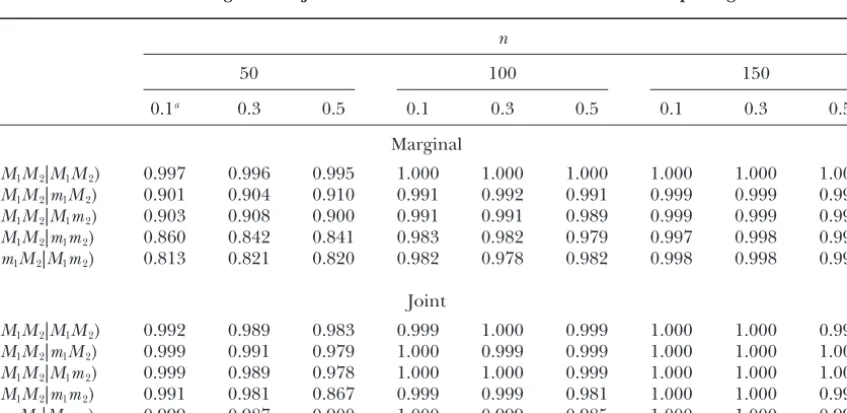
TABLE 3
Estimatedpuni, probability of selecting a unique configuration in the candidate configuration (model)
space, for a tetraploid with two markers, 10,000 simulated data sets, and a cutoff of 0.90 for both the marginal and joint model reduction methods under random pairing
n
50 100 150
0.1a 0.3 0.5 0.1 0.3 0.5 0.1 0.3 0.5
Marginal
(M1M2|M1M2) 0.997 0.996 0.995 1.000 1.000 1.000 1.000 1.000 1.000 (M1M2|m1M2) 0.901 0.904 0.910 0.991 0.992 0.991 0.999 0.999 0.999 (M1M2|M1m2) 0.903 0.908 0.900 0.991 0.991 0.989 0.999 0.999 0.999 (M1M2|m1m2) 0.860 0.842 0.841 0.983 0.982 0.979 0.997 0.998 0.998 (m1M2|M1m2) 0.813 0.821 0.820 0.982 0.978 0.982 0.998 0.998 0.998
Joint
(M1M2|M1M2) 0.992 0.989 0.983 0.999 1.000 0.999 1.000 1.000 0.999 (M1M2|m1M2) 0.999 0.991 0.979 1.000 0.999 0.999 1.000 1.000 1.000 (M1M2|M1m2) 0.999 0.989 0.978 1.000 1.000 0.999 1.000 1.000 1.000 (M1M2|m1m2) 0.991 0.981 0.867 0.999 0.999 0.981 1.000 1.000 0.997 (m1M2|M1m2) 0.999 0.987 0.900 1.000 0.999 0.985 1.000 1.000 0.997
n, sample size.
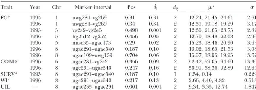
TABLE 4
Estimated locations and effects of QTL associated with winter hardiness and its related traits for autotetraploid alfalfa
Trait Year Chr Marker interval Pos dˆ1 dQ ˆa ˆ FGb 1995 1 uwg284–vg2b9 0.31 0.31 2 12.24, 21.45, 24.61 2.61
1996 1 uwg284–vg2b9 0.34 0.34 2 12.51, 19.18, 19.29 3.17 1995 5 vg2a2–vg2e5 0.498 0.001 2 12.30, 21.65, 23.75 2.82 1996 5 hg2b12–vg2a2 0.456 0.05 2 12.70, 18.48, 22.08 2.96 1996 5 mtsc35–ugac473 0.29 0.02 2 15.23, 18.46, 20.90 3.63 1996 8 ugac291–ugac540 0.187 0.10 2 13.02, 18.60, 21.53 3.08 1996 8 ugac109–uwg169 0.704 0.06 2 15.57, 18.95, 19.95 3.62 CONDc 1996 6 ugac281–vg2c2 0.356 0.09 2 52.42, 59.05, 94.60 13.30 1996 8 ugc291–ugac540 0.247 0.16 2 50.91, 58.36, 92.89 12.64 SURVd 1995 8 ugac291–ugac540 0.187 0.10 1 0.54, 0.14 0.229 WIe 1996 8 ugc291–ugac540 0.217 0.13 2 2.66, 4.40, 4.82 0.513 UIL — 8 ugac235–ugac291 0.001 0.001 2 9.34, 3.35, 12.74 1.847
Data are fromBrouwerandOsborn(1999). Significant QTL were detected by experiment-wise thresholds calculated from 1000 permutation tests at the 0.05 significance level. Chr, chromosome number; Pos, estimated composite map position of the QTL;dˆ1, genetic distance between the detected QTL and left end marker of the interval;dQ, estimated QTL dosage;, estimated common standard deviation of the trait. UIL, unifoliate internode length.
a ⫽(
0,1, . . . ,dQ) is the estimated mean vector.
bThe trait fall growth (FG) was measured by height of vertical regrowth in centimeters in early October in 2 successive years, 1995 and 1996.
cElectrical conductivity per gram fresh weight (COND) was measured in 1995 and 1996 to represent freezing injury (FI).
dWinter survival percentage of plants (SURV) was measured in 1995 and 1996 to represent winter hardiness. eWinter injury (WI) was scaled 1–5 (1, no injury; 5, dead) and was measured in 1996 and 1997.
was crossed to each parent to create two populations of were mapped on chromosome 1, three on
chromo-some 5, and two on chromochromo-some 8. Two pairs of QTL 101 individuals each. Both populations were scored for
82 SDRF loci and measured for each trait in 2 years were detected at close map positions across 2 years: on chromosome 1, one QTL was detected at 0.31 M for of replicated field trials. The composite map and the
original analysis of the trait data and marker data can the 1995 average and one at 0.34 M for the 1996 average; on chromosome 5, one QTL was detected at 0.498 M
be found inBrouwerandOsborn(1999) and
Brou-weret al.(2000). On the basis of the genetic map, seven for the 1995 average and one at 0.456 M for the 1996
average. Two QTL were detected on chromosomes 6 and linkage groups were identified and corresponded to
seven out of the eight chromosomes. As such in what 8 for freezing injury FI. One QTL was detected on chro-mosome 8 for SURV and WI. On chrochro-mosome 8, in the follows, the terms for chromosome and linkage group
are used interchangeably. region from 0.187 to 0.247 M, four QTL were detected
for multiple traits, fall growth (FG 1996), freezing injury Because only B17 markers were considered for the
P13⫻ F1 backcross population and similarly only P13 (COND 1996), winter hardiness (SURV 1995), and win-ter injury (1996); and two of them were at the same lo-markers for the B17 ⫻ F1 backcross, each backcross
population is equivalent to a pseudo-doubled backcross cation, 0.187 M. The one QTL for UIL in the P13 back-cross was at the top of chromosome 8. All of the detected population. Our approach was applied to identify
re-gions in the genome related to the previously described QTL were identified to have dosage two, except for the QTL for winter hardiness (SURV). In general, an addi-quantitative traits for both backcross populations based
on the composite map. The average over the replicates tional copy of a QTL was found to be associated with a higher quantitative trait mean, except for the QTL for in each year for each measurement was treated as a
quantitative trait, and the two averages were analyzed SURV and UIL.
Brouweret al. (2000) used a regression-based single-separately. A permutation test (ChurchillandDoerge
1994) with 1000 permutations for a 0.05 significance marker analysis to identify markers associated with the previously described quantitative traits. Multiple regres-level was used to detect a significant QTL.
Seven QTL were detected for FG, two for FI, one for sion analyses were performed using the same data for all 82 SDRFs to identify the best polygenic models for SURV, and one for WI in the backcross to B17; and
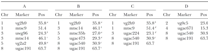
TABLE 5
Estimated locations of QTL affecting traits related to winter hardiness in Brouweret al. (2000): (A) fall growth (FG) 1995 average; (B) fall growth (FG) 1996 average; (C) freezing injury
(FI: COND) 1996 average; (D) winter injury (WI) 1996 average
A B C D
Chr Marker Pos Chr Marker Pos Chr Marker Pos Chr Marker Pos
1 vg2b9 35.8a 1 vg2b9 35.8a 1 vg2b9 35.8b 2 vg0c5 23.0c 1 mtsc9 51.4 3 mtsc14 46.1b 1 mtsc9 51.4d 4 ugac671 15.3 3 uwg96 24.3b 5 mtsc35b 27.0a 3 ugac224 23.1d 8 ugac540 30.9d 3 mtsc14 46.1c 5 ugac473 29.3a 8 ugac540 30.9c 8 ugac191 63.7 5 vg2a2 49.8a 8 ugac540 30.9c 8 ugac191 63.7
8 ugac191 63.7 8 ugac191 63.7c
Chr, chromosome; Pos, estimated composite map position of the QTL. aLocus close to the QTL identified by the interval-mapping method. bLRT at this locus is a peak close to the 0.05 threshold.
cLRT at this locus is higher than the 0.05 threshold, but not a peak. dLRT at this locus is a peak, not close to the 0.05 threshold.
clude six SDRFs for FG (1995), six for FG (1996), five for FI and four QTL for winter injury on chromosomes 1, 5, and 8. The specifics of theMaet al.(2002) method and (COND 1996), and four for WI (1996) [Table 5,
summa-rized fromBrouweret al.’s (2000) Table 2]. Among all analysis make a direct comparison between our results and their results difficult for the following reasons. First, the detected SDRFs, all but five are located on
chromo-somes 1, 5, and 8, which also contain most of QTL we it is assumed inMaet al.(2002) that the markers and QTL have the same dosage level and are in coupling, detected with the proposed method. Two loci for FG
(1995) and three for FG (1996) are also shared by our while most of our detected QTL were of dosage two. Second, there is some evidence that the preferential interval-mapping method. Among the other significant
marker loci, four had likelihood-ratio test statistics pairing factor estimation process provided byMa et al.
(2002) is flawed since in reality the genotypic infor-larger than the 0.05 experiment-wise threshold used in
our interval-mapping method, but were not local peaks. mation collected for across years should not change, yet their estimates of preferential factor do (Caoet al.
Five loci had likelihood-ratio test statistics being local
peaks, with two of them close to the 0.05 threshold. 2004). Finally, inMaet al.(2002) the critical value for the significance level 5% is calculated on the basis of 200 Using an experiment-wise threshold based on a
sig-nificance level 0.05, rather than an asymptotic-based permutation tests. For a 5% significance level (Churchill
and Doerge1994;Doergeand Churchill1996), 200 strict cutoff based on a significance level 0.05 or 0.005
for each marker (Brouwer et al. 2000), we detected permutations limit full exploration of the null space and may lead to the declaration of some QTL that are fewer QTL by controlling the type I error. The region
on chromosome 8 (from 0.187 to 0.247 M) that was actually not significant at the 5% level. identified by our method as being shared by multiple
traits was not detected by the regression method. This
SIMULATION
is most likely the direct result of more experimental
information being incorporated into the analysis (e.g., We used the framework provided by both the alfalfa experiment and analysis as a means to investigate the model selection, dosages, intermarker position). Since
single-marker analysis explores only the relationship be- reliability of the detected QTL via a simulation study. Data were simulated by treating the estimated parental tween the quantitative trait and marker loci, if the QTL
is very close to a marker locus, the estimated effect for configuration and related parameters as the true values. For this purpose, 5 of the 12 QTL that we detected were that marker locus could be interpreted as the effect of
the QTL, under the assumption that the QTL is also of chosen to provide a range for the flanking marker ge-netic distance and configuration, QTL dosage and con-a single dose con-and in coupling with the mcon-arker. However,
most of the QTL that were detected using our method figuration, QTL effect, and QTL position (Table 6). The flanking marker distances were 0.358, 0.358, 0.098, 0.222, were of dosage two; therefore, it is not appropriate to
compare the QTL effects estimated by Brouweret al. and 0.087 M for the five intervals (Table 6). The flanking markers in the first two intervals were in repulsion, and (2000) with our method.
Ma et al. (2002) analyzed the same alfalfa data for the others were in coupling. The estimated QTL dosage
was one for the fourth interval and two for the other two traits, WI and fall injury (FI: COND). They identified
TABLE 6
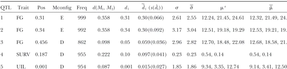
Estimated QTL location and effect for data simulated from five intervals containing detected QTL as indicated by alfalfa data and analysis
QTL Trait Pos Mconfig Freq d(M1,M2) d1 dˆ1(s(dˆ1)) ˆ a ˆ 1 FG 0.31 E 999 0.358 0.31 0.30(0.066) 2.61 2.55 12.24, 21.45, 24.61 12.32, 21.49, 24.54
2 FG 0.34 E 992 0.358 0.34 0.30(0.092) 3.17 3.04 12.51, 19.18, 19.29 12.53, 19.21, 19.29
3 FG 0.456 D 862 0.098 0.05 0.059(0.036) 2.96 2.82 12.70, 18.48, 22.08 12.68, 18.58, 21.89
4 SURV 0.187 D 955 0.222 0.10 0.097(0.041) 0.23 0.23 0.54, 0.14 0.54, 0.14
5 UIL 0.001 D 954 0.087 0.001 0.015(0.027) 1.85 1.86 9.34, 3.35, 12.74 9.14, 3.41, 12.50
For each interval, 1000 data sets of sample size 100 were simulated. Pos, position of the detected QTL on the composite genetic map; Mconfig, marker configuration (D is coupling and E is repulsion);d1, distance between the QTL and the left end marker;, common standard deviation of the trait for all QTL dosage levels; Freq, frequency of selecting the correct parental configuration out of 1000 data sets;dˆ1, average of the 1000 estimated QTL locations from the 1000 simulated data sets;s(dˆ1), sample standard deviation of the 1000 estimated QTL locations from the 1000 simulated data sets;ˆ, average of population standard deviation estimates;ˆ , average of population mean vector estimates.
a ⫽(
0,1, . . . ,dQ) is the mean vector of the trait corresponding to QTL dosages.
was similar to that of the first interval. We included the QTL can be provided by this extra copy of the QTL. This, in turn, makes it difficult to choose between the second interval in our simulation because we were
inter-ested in investigating whether our method is able to configurations with one copy and two copies of the QTL. On the other hand, with markers in repulsion, both identify the small increment from1to2, where⫽
(0, 1, 2) ⫽ (12.51, 19.18, 19.29) is the estimated copies of the QTL provide information about recombi-nation between markers and QTL. The effect of this dif-mean vector for the corresponding QTL in that interval.
The five interval settings were studied separately. For ference is easily illustrated by comparing the second interval with the third interval used for this simulation. each interval, 1000 data sets with a sample size of 100
(i.e., similar to the alfalfa data) were simulated and ana- Although the increment in trait means from QTL dose 1 to dose 2 is only 0.035for case 2 and 1.22for case 3, lyzed, with results summarized in Table 6. Using the joint
model selection method, the correct parental marker con- case 2 still outperformed case 3. On the basis of this, repulsion is not necessarily the worst-case scenario for figuration was included in the candidate parental marker
configuration pool 100% of the time for all five cases. QTL mapping in tetraploids with simplex markers, as was once thought.
The overall parental configuration pool is then formed
by the combination of candidate parental marker config- Since the above simulation was mainly focused on pa-rental marker configurations formed by simplex mark-urations and possible QTL configmark-urations. After fitting our
interval-mapping model to each possible parental con- ers, another simulation study was performed to serve as the basis of investigation for how, in general, QTL or figuration, the one having the maximal test statistic
pro-vides the estimated QTL location and marker and QTL marker dosages and their respective linkage phase af-fect the performance of our algorithm. Under a pseudo-configuration, as well as the parameter estimates. The
cor-rect configuration was identified at least 95% of the time doubled backcross experiment, two markers (M1/m1and
M2/m2) and one QTL (Q/q) were used with marker with markers in coupling and at least 99% of the time with
markers in repulsion, except for the third interval where distance 0.10 M and a sample size 100. The location of the QTL was 0.01, 0.03, or 0.05 M. The trait mean the correct configuration was selected 86% of the time.
Given the correct configuration, the estimated parame- was (10.0, 12.0) if QTL dosage was 1 or (10.0, 12.0, 14.0) if QTL dosage was 2, and was 1.0. One thou-ters were close to the true values used for simulation.
The fact that our method performed better with re- sand data sets were simulated for each combination of the parameter settings and each of the following con-pulsion than with coupling is due to the difference
between these two configurations. This can be demon- figurations: double coupling (A1, A3), asymmetric cou-pling 12 (B1, B2, B3), coucou-pling (D1, D2, D3), and repul-strated by considering an example where two copies of
the QTL are on both informative chromosomes. When sion (E1, E2, E3).
Our simulation results illustrate that when the correct the markers are in coupling, one copy of the QTL is
located on a chromosome containing no dominant parental configuration was identified, the parameter
estimate averages were close to the true value. The abil-marker alleles. Thus, not much extra information with
de-mizing the disequilibrium in pairing. However, with ran-dom pairing, one-third of the time one informative chro-mosome pairs with another informative chrochro-mosome to provide less, or even no, information, if two chromo-somes are homozygous. Using similar reasoning it can be demonstrated that random pairing is more informa-tive than preferential pairing for markers in repulsion.
DISCUSSION
One of the largest challenges when mapping QTL in polyploids is the incomplete parental configuration (model) information. This is compounded by the dra-matic increase in the size of the model space as the number of markers and/or ploidy level increase. To
Figure3.—The proportion identifying the correct parental
(marker and QTL) configuration for a tetraploid under a combat these challenges in autopolyploid QTL
map-pseudo-doubled backcross experiment. The trait mean is ping, our interval-mapping algorithm takes one of two (10.0, 12.0) if QTL dosage is 1 or (10.0, 12.0, 14.0) if QTL approaches. The size of the model space is addressed dosage is 2. Population standard deviationis 1.0. With
sam-using Bayesian model selection by first identifying
po-ple size 100, 1000 data sets are simulated under 11 parental
tential parental marker dosages using a marginal
ap-configurations corresponding to numbers 1–11 on the
hori-zontal axis: A1, A3, B1, B2, B3, D1, D2, D3, E1, E2, and E3. proach or marker configurations based on a joint
ap-The letters denote the marker configurations: (A) double proach. We have demonstrated that both methods are coupling, (B) asymmetric coupling 12, (D) coupling, and (E) effective in reducing the model space, but that the joint repulsion. The numbers denote the QTL configurations: (1)
method is more efficient due to the fact that it
incorpo-one dose of QTL present on the first informative chromosome,
rates the genetic map information. From the reduced
(2) one dose of QTL present on the second informative
chro-mosome, and (3) two doses of QTL present on both informa- model space, the candidate parental configuration pool
tive chromosomes.d(M1,Q) is the genetic distance between is formed by combining each potential parental marker the QTL and the left end-flanking marker. configuration with a possible QTL configuration. For
each potential parental configuration, profiles of MLEs of QTL effects, as well as population variation and likeli-pended on the underlying parental configuration. The hood-ratio test statistics, are produced at each evalua-worst-case scenario was when markers were in coupling tion point of a grid search across the genome. Putative on the first informative chromosome with one copy of QTL are detected using a resampling-based significance
the QTL on the second informative chromosome (D2). threshold. The corresponding parental configuration
For this case the identified correct configuration pro- (and related parameter estimates) is then taken as the portion ranged from 63 to 66% (Figure 3). This is not underlying model from which the data are produced. surprising since with D2 under random pairing, only Our simulation studies have demonstrated that if the one-third of the pairings provide information concern- correct parental configuration is identified, our
interval-ing the recombination between marker and QTL. On mapping method provides parameter estimates close
the other hand, the best situation was when two markers to true values. However, the chance of identifying the were in repulsion, where the correct parental configu- correct configuration depends on the true parental con-ration was almost 100% regardless of the QTL configu- figuration, chromosome pairing system, and genetic dis-ration or location. Most of the other configudis-rations ob- tance between markers and the QTL. This helps us
tained a proportion of at least 95% (Figure 3). address a question raised inDoergeandCraig(2000,
It is worth noting that in our earlier work (Caoet al. p. 7956), “for which situation is the linkage mostly
af-2003), repulsion did not outperform configurations with fected?” Comparatively, among these factors, the true higher dosages of loci, such as double coupling and asym- parental configuration is the most influential one. Since metric coupling. The difference in results comes from a configuration consists of both loci dosages and linkage the difference in the assumed chromosome-pairing mech- phase, the influence of one cannot be considered with-anism. Our earlier work (Caoet al.2003) investigated out considering the effect of the other. For example, a
the performance of our interval-mapping method un- configuration with higher marker/QTL dosages does
maxi-tive to the chromosome-pairing system and thus con- sumption does not hold, we can simply change the upper
sistently provides high power for detecting QTL. bound for the QTL dosage to the ploidy level. This
Our simulation results also help to answer some of the change will result in more candidate QTL configura-remaining questions presented byDoerge andCraig tions to choose from, but the method and the procedure (2000, p. 7956). First, “If a molecular marker is found remain the same. Similarly, if the breeding design is
to be tightly linked to a QTL, should the dosage of altered from a pseudo-doubled backcross design, our
the marker agree with the dosage of the QTL?” Not approach can be adapted. Also, if codominant markers
necessarily. There is no causal relationship between the are considered, they can be easily incorporated in the dosages of the QTL and the flanking markers. Although model by including parameters such as allelic effect and as discussed previously a configuration with the marker interaction.
and QTL having the same dosage often has a higher The effect of the assumptions we place on the genetic
disequilibrium and thus a higher power of detecting map that is used for QTL mapping in polyploids is one QTL. Second, “Should the models which are controlled area of research that remains unaddressed. When the by dosage levels be weighted for the purpose of repre- genetic map is estimated, the most likely parental marker senting more realistic results?” Weighting the candidate configuration in turn has to be estimated since recombi-models may be a better way than depending solely on nation requires a parental marker configuration. Be-the one “best” model, when Be-the uncertainty about pa- cause of this, the parental marker configuration used rental configuration is high. However, even configura- for estimating the genetic map should be consistent tions with the same marker dosage levels could differ with the one used to locate QTL. However, if the most to a greater extent biologically; therefore, further inves- likely parental marker configuration is not the correct tigation is needed to find a both statistically and biologi- configuration, the reliability of the map and the mapped cally sound weighting scheme. Finally, “Would models QTL are affected. By selecting the pool of potential pa-with dosage levels more similar to each other be more rental configurations on the basis of observed progeny likely, especially with close linkage (short genetic dis- data, our method can serve as a further verification for tance)?” This answer depends on the linkage phase the estimated genetic map. A framework is currently under since it is possible for two models with exactly the same development to allow variability or uncertainty in estimat-dosage levels and genetic association to be biologically ing the map to be considered when mapping QTL. different due to different linkage phases, and therefore
We thank Tom Osborn for providing the data set and continued
they are different in likelihood. work in this area, and we thank Gary Churchill for his comments on
We applied our approach to a published alfalfa data this work.
set for quantitative traits that are related to winter hardi-ness. Our analysis confirms several putative QTL identi-fied by a regression-based single-marker analysis (
Brou-LITERATURE CITED
weret al.2000), and it also identified a new region on
Bayes, T., 1783 An essay towards solving a problem in the doctrine
chromosome 8 that was shared by several traits. Our
of chances. Philos. Trans. R. Soc. Lond.53:370–418.
analysis results demonstrate that for a majority of the
Bingham, E. T., andT. J. McCoy, 1988 Cytology and cytogenetics
detected QTL, there is a positive or negative correlation of alfalfa, pp. 737–776 inAlfalfa and Alfalfa Improvement, edited by A. A.Hanson, D. K.Barnesand R. R.Hill, Jr. American
between the quantitative trait mean and QTL dosage
Society of Agronomy, Madison, WI.
level;i.e.,0ⱕ 1ⱕ. . .ⱕ dQor0ⱖ 1ⱖ. . .ⱖ dQ.
Broman, K. W., 2001 Review of statistical methods for qtl mapping
If such an ordering of means is available before analysis, in experimental crosses. Lab Anim.30(7): 44–52.
Brouwer, D., andT. Osborn, 1999 A molecular marker linkage
an order-restricted version of interval mapping can be
map of tetraploid alfalfa. Theor. Appl. Genet.99:1194–1200.
performed to improve power of detection. With an
or-Brouwer, D. J., S. H. Dukeand T. C. Osborn, 2000 Mapping
der constraint, the problem falls into the category of genetic factors associated with winter hardiness, fall growth, and
freezing injury in autotetraploid alfalfa. Crop Sci.40:1387–1396.
isotonic regression and it can be computed using the
Cao, D., B. A. CraigandR. W. Doerge, 2003 Interval mapping for
pool-adjacent-violator algorithm (Robertsonet al.1988).
autopolyploids, pp. 60–72 inProceedings of the 15th Annual Kansas We have performed simulations (not shown) to com- State University Conference on Applied Statistics in Agriculture, edited pare the power between an order restriction and without by G.Milliken. Kansas State University, Manhattan, KS.
Cao, D., T. C. OsbornandR. W. Doerge, 2004 Correct estimation
one. In fact, even when the only information is that the
of preferential chromosome pairing in autotetraploids. Genome
means are ordered, and the direction remains un- Res.14:459–462.
known, there is a slight improvement in the perfor- Churchill, G. A., and R. W. Doerge, 1994 Empirical threshold values for quantitative trait mapping. Genetics138:963–971.
mance. The improvement is most evident when the order
Darlington, C. D., 1931 Meiosis in diploid and tetraploid primula
of the means is increasing or decreasing with respect to sinensis. J. Genet.24:65–98.
the QTL dosage and is knowna priori. Dempster, A. P., N. M. LairdandD. B. Rubin, 1977 Maximum
likelihood from imcomplete data via the em algorithm. J. R. Stat.
Thus far it has been assumed that the QTL dosage
Soc. Ser. B39(1): 1–38.
is at most half the ploidy level, which is a reasonable
Dietrich, W. F., J. Miller, R. Steen,M. A. Merchant, D. Damron-assumption given the pseudo-doubled backcross experi- Boleset al., 1996 A comprehensive genetic map of the mouse
genome. Nature380:149–152.
as-Doerge, R. W., 2002 Mapping and analysis of quantitative trait loci Ma, C.-X., G. Casella, Z.-J. Shen, T. C. OsbornandR. Wu, 2002 A unified framework for mapping quantitative trait loci in bivalent in experimental populations. Nat. Rev. Genet.3:43–52.
tetraploids using single-dose restriction fragments: a case study
Doerge, R. W., andG. A. Churchill, 1996 Permutation tests for
from alfalfa. Genome Res.12:1974–1981. multiple loci affecting a quantitative character. Genetics142:285–294.
Mather, K., 1938 Crossing-over. Biol. Rev.13:252–292.
Doerge, R. W., andB. A. Craig, 2000 Model selection for
quantita-Muller, H. J., 1916 The mechanism of crossing-over. Am. Nat.50
tive trait locus analysis in polyploids. Proc. Natl. Acad. Sci. USA
(592): 193–221, 284–305, 350–366, 421–434.
97(14): 7951–7956.
Newton, W. C. F., andC. D. Darlington, 1929 Meiosis in
poly-Doerge, R. W., Z-B. ZengandB. S. Weir, 1997 Statistical issues in
ploids. J. Genet.21:1–56. the search for genes affecting quantitative traits in experimental
Osborn, T., J. Pires, J. Birchler,D. L. Auger, Z. J. Chenet al., populations. Stat. Sci.12(3): 195–219.
2003 Understanding mechanisms of novel gene expression in
Grattapaglia, D., andR. Sederoff, 1994 Genetic linkage maps
polyploids. Trends Genet.19(3): 141–147. of eucalyptus grandis and eucalyptus urophylla using a
pseudo-Rieseberg, L. H., andM. F. Doyle, 1989 Tetrasomic segregation testcross: mapping strategy and RAPD markers. Genetics137:
in the naturally occurring autotetraploidallium nevii(aliaceae). 1121–1137.
Hereditas111:31–36.
Hackett, C. A., J. E. BradshawandJ. W. McNicol, 2001 Interval
Ripol, M., G. Churchill, J. da SilvaandM. Sorrells, 1999 Statisti-mapping of quantitative trait loci in autotetraploid species.
Genet-cal aspects of genetic mapping in autopolyploids. Gene 235:
ics159:1819–1832. 31–41.
Haley, C. S., andS. A. Knott, 1992 A simple regression method Robertson, T., F. T. WrightandR. L. Dykstra, 1988 Order Re-for mapping quantitative trait loci in line crosses using flanking stricted Statistical Inference, Ed. 1. Wiley, New York.
markers. Heredity69:315–324. Rodzen, J. A., andB. May, 2002 Inheritance of microsatellite loci
Jackson, R. C., andJ. W. Jackson, 1996 Gene segregation in auto- in the white sturgeonacipenser transmontanus.Genome45:1064–1076. tetraploids: prediction from meiotic configurations. Am. J. Bot. Soltis, D. E., andP. S. Soltis, 1999 Polyploidy: recurrent formation
83(6): 673–678. and genome evolution. Trends Ecol. Evol.14(9): 348–352.
Jansen, R. C., 1993 Interval mapping of multiple quantitative trait Soltis, D. E., P. E. SoltisandJ. A. Tate, 2003 Advances in the study loci. Genetics135:205–211. of polyploidy since plant speciation. New Phytol.161:173–191.
Knapp, S. J., J. W. C. BridgesandD. Brikes, 1990 Mapping quantita- Soltis, P. S., andD. E. Soltis, 2000 The role of genetic and genomic attributes in the success of polyploids. Proc. Natl. Acad. Sci. USA tive trait loci using molecular marker linkage maps. Theor. Appl.
97(13): 7051–7057. Genet.79:583–592.
Suzuki, D. T., A. J. F. Griffiths, J. H. MillerandR. C. Lewontin,
Koornneef, M., J. van Eden, C. J. Hanhart,P. Stam, F. J. Braaksma
1989. Introduction to Genetics, Ed. 4. W. H. Freeman, New York.
et al., 1983 Linkage map ofarabidopsis thaliana.J. Hered.74:
Sybenga, J., 1995 Meiotic pairing in autohexaploidlathyrus: a math-265–272.
ematical model. Heredity75:343–350.
Lander, E. S., andD. Botstein, 1989 Mapping Mendelian factors
Wolfe, K. H., 2001 Yesterday’s polyploids and the mystery of dip-underlying quantitative traits using RFLP linkage maps. Genetics
loidization. Nat. Rev. Genet.2:333–341.
121:185–199.
Wu, K. K., W. Burnquist, M. Sorrells, T. L. Tew, P. H. Mooreet al.,
Luo, Z. W., C. A. Hackett, J. E. Bradshaw, J. W. McNicoland
1992 The detection and estimation of linkage in polyploids
D. Milbourne, 2000 Predicting parental genotypes and gene
using single-dose restriction fragments. Theor. Appl. Genet.83:
segregation for tetrasomic inheritance. Theor. Appl. Genet.100:
294–300. 1067–1073.
Zeng, Z-B., 1993 Theoretical basis for separation of multiple linked
Luo, Z. W., C. A. Hackett, J. E. Bradshaw, J. W. McNicolandD. Mil- gene effects in mapping quantitative trait loci. Proc. Natl. Acad. bourne, 2001 Construction of a genetic linkage map in tetraploid Sci. USA90(23): 10972–10976.
species using molecular markers. Genetics157:1369–1385. Zeng, Z-B., 1994 Precision mapping of quantitative trait loci.
Genet-Luo, Z. W., R. ZhangandM. J. Kearsey, 2004 Theoretical basis ics136:1457–1468. for genetic linkage analysis in autotetraploid species. Proc. Natl.