R E S E A R C H
Open Access
Two species competitive model with the
Allee effect
Ann Brett and Mustafa RS Kulenovi´c
**Correspondence:
kulenm@math.uri.edu Department of Mathematics, University of Rhode Island, Kingston, RI 02881-0816, USA
Abstract
We consider the following system of difference equations:xn+1= ax 2 n 1+x2n+cyn, yn+1= by
2 n
1+yn2+dxn,n= 0, 1,. . ., wherea,b,c,dare positive constants andx0,y0≥0 are
initial conditions. This system has interesting dynamics and can have up to nine equilibrium points. The most complex and perhaps most interesting case is the case of nine equilibrium points, four of which are local attractors, four of which are saddle points, and one of which is a repeller. Using recent results of Kulenovi´c and Merino we are able to characterize the basins of attractions of all local attractors and thus to describe the global dynamics of this system. This case can be considered as a two-dimensional version of the Allee effect for competitive systems.
MSC: 39A10; 39A30; 37G35
Keywords: Allee effect; basin; competition; difference equation; global asymptotic stability; invariant manifold; stable manifold
1 Introduction
The following difference equation is known as the Beverton-Holt model:
xn+= axn
+xn
, n= , , . . . , ()
wherea> is the rate of change (growth or decay) andxnis the size of the population at
thenth generation.
This model was introduced by Beverton and Holt in . It depicts density depen-dent recruitment of a population with limited resources which are not shared equally.
The model assumes that theper capitanumber of offspring is inversely proportional to a
linearly increasing function of the number of adults. In other words () can be considered as an equation of the form
xn+=xnf(xn), n= , , . . . , ()
wheref(u) =a/( +u) is inversely proportional to the linear functionA+Bu,A,B> ,
which can be normalized to be +u.
The Beverton-Holt model is well studied and understood. It exhibits the following prop-erties.
Theorem Equation()has the two equilibrium pointsand a– when a> .
(a) All solutions of()are monotonic(increasing or decreasing)sequences.
(b) Ifa≤,then the zero equilibrium is a global attractor,that is,limn→∞xn= ,for all x≥.
(c) Ifa> ,then the equilibrium pointa– is a global attractor,that is,
limn→∞xn=a– ,for allx> .
(d) Both equilibrium points are globally asymptotically stable in the corresponding regions of parametersa≤anda> ,that is,they are global attractors with the property that small changes of initial conditionxresult in small changes of the corresponding solution{xn}.
Furthermore, () can be solved explicitly and has the following solution:
xn=
/(a– ) + (/x– /(a– ))/an
ifa= ,
xn=
n+ /x
ifa= ,
()
which can be used to prove all the preceding properties. See [–].
The Allee effect is a phenomenon in biology characterized by a positive correlation
be-tween population density andper capitagrowth rate. The Allee effect was first written on
extensively by its namesake Warder Clyde Allee. The general idea of the Allee effect is that for smaller populations, the reproduction and survival rates of individuals decrease. This effect usually saturates or disappears as populations get larger. The Allee effect has been detected in a number of discrete models; see [–].
The effect may be due to any number of causes. In some species, reproduction (finding a mate in particular) may be increasingly difficult as the population density decreases.
In mathematics, when the basin of attraction of the zero equilibrium of a system contains an open set, we consider the system to exhibit the Allee effect. See [, ].
In view of Theorem the Beverton-Holt model does not exhibit the Allee effect.
1.1 Beverton-Holt type model that exhibits the Allee effect The difference equation
xn+= axn
+x n
, n= , , . . . , ()
which was introduced by Thompson [] as a depensatory generalization of the Beverton-Holt stock-recruitment relationship, was used to develop a set of constraints designed to safeguard against overfishing. This model has been used in the study of fish population dynamics, particularly when overfishing is present; see [] for further references. In view of the sigmoid shape of the functionf(u) =+uau, () is called the sigmoid Beverton-Holt
model. A very important feature of the sigmoid Beverton-Holt model is that it exhibits the Allee effect. We can see this from the following result, the proof of which is an immediate consequence of a stair-step diagram analysis.
(a) Equation()has only a zero equilibrium whena< .
(b) Equation()has a zero equilibrium and the positive equilibriumx¯= /,whena= . (c) There exists a zero equilibrium and two positive equilibria,x¯–andx¯+,whena> .
(d) All solutions of()are monotonic(increasing or decreasing)sequences.
(e) Ifa< ,then the equilibrium pointis a global attractor,that is,limn→∞xn= for allx≥.
(f ) Ifa= ,then the equilibrium pointis a global attractor,with the basin of attraction B() = (,x¯)andx¯= /is a non-hyperbolic equilibrium point with the basin of attractionB(x¯) = [x¯,∞).
(g) Ifa> ,then we have zero equilibrium andx¯+are locally asymptotically stable,while ¯
x–is a repeller and the basins of attraction of the equilibrium points are given as
B() ={x: ≤x<x¯–},
B(x¯+) ={x:x¯–<x<∞}.
In other words,the smaller positive equilibrium serves as the boundary between two basins of attraction.The zero equilibrium has the basin of attractionB()and the model exhibits the Allee effect.
(h) The equilibrium pointsandx¯+are globally asymptotically stable in the corresponding basins of attractionsB()andB(x¯+).
1.2 Competitive model in two dimensions that exhibits the Allee effect
We will now consider the two-dimensional analog of () which is the uncoupled system
xn+= ax
n
+x n
,
yn+= by
n
+y n
, n= , , . . . ,
()
where aandbare positive parameters. System () can have at most nine nonnegative
equilibrium points:
E(, ), E¯y–(,y¯–), E¯y+(,y¯+),
E¯x–(x¯–, ), E¯x+(x¯+, ), E–(x¯–,y¯–),
E–+(x¯–,y¯+), E+–(x¯+,y¯–), E+(x¯+,y¯+).
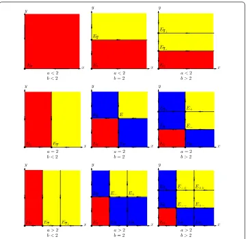
The dynamics of system () is partially described in the following theorem, with com-plete visual interpretation in Figure can be derived from Theorem . Since there are three dynamics scenarios for each of two equations in (), there are nine dynamic scenarios for system (), which are visualized in Figure .
Theorem System()has the following properties:
(a) All solutions(xn,yn)of system()are component-wise monotonic and bounded,that is,both sequences{xn}and{yn}are monotonic and bounded.
Figure 1 Global dynamics of uncoupled two-dimensional model()with nine dynamics scenarios.
(c) Ifa< ,b> ,then the basins of attraction of the equilibrium points are given as BE(, )
=(x,y) : ≤x<∞, ≤y<y¯–
,
BE¯y+(,y¯+)
=(x,y) : ≤x<∞,y¯–<y<∞
.
(d) Ifa> ,b< ,then the basins of attraction of the equilibrium points are given as BE(, )
=(x,y) : ≤x<x¯–, ≤y<∞
,
BE¯x+(x¯+, )
=(x,y) :x¯–<x<∞, ≤y<∞
.
(e) Ifa> ,b> ,then the basins of attraction of the equilibrium points are given as BE(, )
=(x,y) : ≤x<x¯–, ≤y<y¯–
,
BE¯x+(x¯+, )
=(x,y) :x¯–<x<∞, ≤y<y¯–
,
BE¯y+(,y¯+)
=(x,y) : ≤x<x¯–,y¯–<y<∞
,
BE++(x¯+,¯y+)
=(x,y) :x¯–<x<∞,y¯–<y<∞
,
BE¯x–(x¯–, )
=(x¯–,y) : ≤y<¯y–
BE¯y–(,y¯–)
Two species can interact in several different ways through competition, cooperation, or predator-prey interactions. For each of these interactions, we obtain variations of system (), all of which may require a different mathematical analysis.
equilibrium points in the hyperbolic case and two, four, six or eight equilibrium points in the non-hyperbolic case. In each of these cases we will show that the Allee effect is present and we will precisely describe the basins of attraction of all equilibrium points. We will show that the boundaries of the basins of attraction of the equilibrium points are the global stable manifolds of the saddle or the non-hyperbolic equilibrium points. See [–] for related results. An interesting feature of our results is that the size of the basin of attraction of the zero equilibrium decreases as a function of the number of the equilibrium points. The biological interpretation of our results is given in [, ] and a similar system is treated in []. However, no details of the proofs are provided in [, ] and non-hyperbolic cases were not treated there. Here we give the detailed proofs of all dynamic scenarios and provide the explicit algebraic conditions for the existence of one through nine equilibrium points, which was also missing in [, ]. A specific feature of our results is that no equilibrium point in the interior of the first quadrant is computable and so our analysis is based on the geometry of the equilibrium curves.
2 Preliminaries
Our proofs use some recent general results for competitive systems of difference equations of the form
xn+=f(xn,yn), yn+=g(xn,yn),
()
where f and g are continuous functions and f(x,y) is non-decreasing in x and
non-increasing inyandg(x,y) is non-increasing inxand non-decreasing inyin some domainA. Competitive systems of the form () were studied by many authors in [, , –] and others.
Here we give some basic notions as regards monotonic maps in a plane.
We define apartial orderseonR(the so-called southeast ordering) so that the positive
cone is the fourth quadrant,i.e., this partial order is defined by
Similarly, we define northeast ordering as
A mapFis calledcompetitiveif it is non-decreasing with respect tose, that is, if the
ForS⊂R
+letS◦denote theinteriorofS.
The following definition is from [].
Definition LetRbe a nonempty subset ofR. A competitive mapT:R→Ris said to
satisfy condition (O+) if for everyx,yinR,T(x)neT(y) impliesxney, andT is said to satisfy condition (O–) if for everyx,yinR,T(x)neT(y) impliesynex.
The following theorem was proved by de Mottoni-Schiaffino [] for the Poincaré map of a periodic competitive Lotka-Volterra system of differential equations. Smith general-ized the proof to competitive and cooperative maps [, ].
Theorem Let R be a nonempty subset ofR.If T is a competitive map for which(O+)
holds then for all x∈R,{Tn(x)}is eventually component-wise monotone.If the orbit of x has compact closure,then it converges to a fixed point of T.If instead(O–)holds,then for all x∈R,{Tn}is eventually component-wise monotone.If the orbit of x has compact closure in R,then its omega limit set is either a period-two orbit or a fixed point.
It is well known that a stable period-two orbit and a stable fixed point may coexist; see Hess [].
A non-hyperbolic equilibrium pointEof a competitive or cooperative mapTis called
non-hyperbolic point of stable type (resp. of unstable type) if the second characteristic value of the Jacobian matrixJT(E) is in interval (–, ) (resp. outside of interval [–, ]).
The following result is from [], with the domain of the map specialized to be the
Carte-sian product of intervals of real numbers. It gives a sufficient condition for conditions (O+)
and (O–).
Theorem Let R⊂Rbe the Cartesian product of two intervals inR.Let T:R→R be a Ccompetitive map.If T is injective anddetJT(x) > for all x∈R then T satisfies(O+).If T is injective anddetJT(x) < for all x∈R then T satisfies(O–).
Theorems and are quite applicable as we have shown in [], in the case of compet-itive systems in the plane consisting of linear fractional equations.
The following result is from [], which generalizes the corresponding result for hyper-bolic case from []. Related results have been obtained by Smith in [].
Theorem LetRbe a rectangular subset ofRand let T be a competitive map onR.Let ¯
x∈Rbe a fixed point of T such that(Q(x¯)∪Q(x¯))∩Rhas nonempty interior(i.e.,x is¯ not the NW or SE vertex ofR).
Suppose that the following statements are true.
(a) The mapTis strongly competitive onint((Q(x¯)∪Q(x¯))∩R).
(b) TisCon a relative neighborhood ofx¯.
(c) The Jacobian ofT atx¯has real eigenvaluesλ,μsuch that|λ|<μ,whereλis stable and the eigenspaceEλassociated withλis not a coordinate axis.
(d) Eitherλ≥and
T(x)=x¯ and T(x)=x for allx∈intQ(x¯)∪Q(x¯)
orλ< and
T(x)=x for allx∈intQ(x¯)∪Q(x¯)
∩R.
Then there exists a curveCinRsuch that:
(i) Cis invariant and a subset ofWs(x¯).
(ii) The endpoints ofClie on∂R. (iii) x¯∈C.
(iv) Cthe graph of a strictly increasing continuous function of the first variable. (v) Cis differentiable atx¯ifx¯∈int(R)or one sided differentiable ifx¯∈∂R,and in all
casesCis tangential toEλatx¯.
(vi) CseparatesRinto two connected components,namely
W–:={x∈R:∃y∈Cwithxy}
and
W+:={x∈R:∃y∈Cwithyx}.
(vii) W–is invariant,anddist(Tn(x),Q(x¯))→asn→ ∞for everyx∈W–.
(viii) W+is invariant,anddist(Tn(x),Q(x¯))→asn→ ∞for everyx∈W+.
The next results from [] give the existence and uniqueness of invariant curves ema-nating from a non-hyperbolic point of unstable type, that is, a non-hyperbolic point where the second eigenvalue is outside the interval [–, ]. See also [].
Theorem LetR= (a,a)×(b,b),and let T:R→Rbe a strongly competitive map with a unique fixed pointx¯∈R,and such that T is continuously differentiable in a neigh-borhood ofx.¯ Assume further that at the pointx¯the map T has associated characteristic valuesμandνsatisfying <μand–μ<ν<μ.
Then there exist curvesC,CinRand there existp,p∈∂Rwithpsex¯sepsuch that:
(i) For= , ,Cis invariant,northeast strongly linearly ordered,such thatx¯∈Cand C⊂Q(x)¯ ∪Q(x)¯ ;the endpointsq,rofC,whereqner,belong to the
boundary ofR.For,j∈ {, }with=j,Cis a subset of the closure of one of the
components ofR\Cj.BothCandCare tangential atx¯to the eigenspace associated withν.
(ii) For= , ,letBbe the component ofR\Cwhose closure containsp.ThenBis
invariant.Also,forx∈B,Tn(x)accumulates onQ(p)∩∂R,and forx∈B, Tn(x)accumulates onQ
(p)∩∂R.
(iii) LetD:=Q(x)¯ ∩R\(B∪B)andD:=Q(x)¯ ∩R\(B∪B).ThenD∪Dis invariant.
Corollary Let a map T with fixed pointx¯be as in Theorem.LetD,Dbe the sets as in Theorem.If T satisfies(O+),then for= , ,Dis invariant,and for everyx∈D,the
3 Main results
The main results of this paper depend on the number of interior equilibrium points of system (). So first we give the explicit algebraic conditions in terms of the parameters for system () to have zero-five interior equilibrium points. Next, we present the local stability analysis of the equilibrium points and then the results on the global dynamics. It is interesting to note that the local stability analysis is the most difficult part of our analysis.
3.1 Equilibrium points
The equilibrium points of system () satisfy the following system of equations:
¯
x= ax¯
+x¯+cy¯,
¯
y= by¯
+y¯+dx¯, n= , , . . . .
()
All solutions of system () with at least one zero component are given asE(, ),E¯x(x¯, )
where x¯= ,E¯y(,y¯) where y¯= ,E¯x±(,x±¯ ) where x±¯ = a± √
a–
, and E¯y±(,y±¯ ) where ¯
y±=b±
√ b–
.E(, ) exists in all cases.E¯x(x¯, ) andE¯y(,y¯) exist whena= andb= ,
respectively.E¯x±(,x±¯ ) andE¯y±(,y±¯) exist whena> andb> , respectively.
The equilibrium points with strictly positive coordinates satisfy the following system of equations:
–ax+cy+x+ = ,
–by+dx+y+ = .
()
From () one can see that all positive solutions of system () satisfy the quartic equation:
x– ax+xa+bc+ +xcd–a(bc+ )+bc+c+ = . ()
Lemma Let
= –a
b– d–a– bc+a– – b– c
– acda– (bc+ )+ da(bc+ ) –acb(bc+ ) – c+
– (bc+ )b– c– bc–
+b– a– a(bc+ ) + c(b+c) + – cd, ()
=
b– a– bc– – ada– bc– – cd ()
and
=a– bc– .
Then the following holds:
(a) If> ,> ,and> ,then()has four simple real roots.
(b) If> and≤∨(> ∧≤)then()has no real roots.
(d) If= and< then()has one real double root.
(e) If= and> then()has two real simple roots and one real double root.
(f ) If= ,= and> then()has two real double roots.
(g) If= ,= and< then()has no real roots.
(h) If= ,= and= then()has one real root of multiplicity four. Proof The discrimination matrix [] off˜andf˜is given by
Discr(f˜)
=
⎛ ⎜ ⎜ ⎜ ⎜ ⎜ ⎜ ⎜ ⎜ ⎜ ⎜ ⎝
–a a+bc+ cd–a(bc+ ) c+bc+
–a (a+bc+ ) cd–a(bc+ )
–a a+bc+ cd–a(bc+ ) c+bc+
–a (a+bc+ ) cd–a(bc+ )
–a a+bc+ cd–a(bc+ ) c+bc+
–a (a+bc+ ) cd–a(bc+ )
–a a+bc+ cd–a(bc+ ) c+bc+
–a (a+bc+ ) cd–a(bc+ )
⎞ ⎟ ⎟ ⎟ ⎟ ⎟ ⎟ ⎟ ⎟ ⎟ ⎟ ⎠ ,
where
˜
f(x) =x– ax+xa+bc+ +xcd–a(bc+ )+bc+c+ .
LetDkdenote the determinant of the submatrix ofDiscr(f˜), formed by the first krows
and the first kcolumns, fork= , , , . So, by straightforward calculation one can see
thatD= ,D= ,D= c, andD=c. The rest of the proof follows in view of
[, Theorem ].
3.2 Local stability of equilibrium points
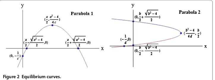
Geometrically the solutions of system () are intersections of two orthogonal parabolas that satisfy the equations
y= –
c
x–a
+a
–
c ,
x= –
d
y–b
+b
–
d ,
()
with respective vertices (a,ac–) and (bd–,b). See Figure .
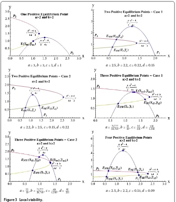
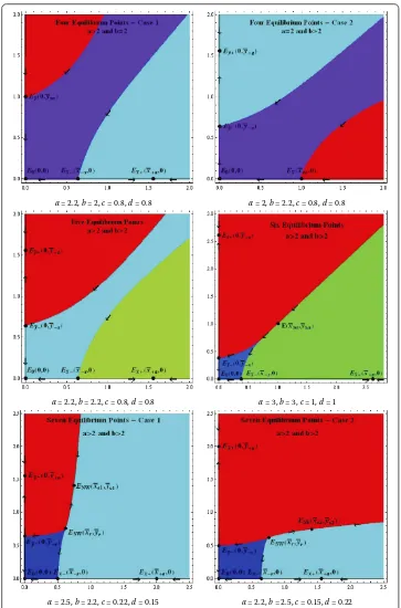
Consequently whena> andb> , in addition to the five equilibrium points on the axes, system () may have one, two, three or four positive equilibrium points. We will refer to these equilibrium points asESW(x¯,y¯) (southwest),ESE(x¯,y¯) (southeast),ENW(x¯,¯y)
(northwest), andENE(x¯,y¯) (northeast) where
ENWseENEseESE, ESWneENW.
When a positive equilibrium point is non-hyperbolic we will refer to it asEN(x¯,y¯).
The map associated with system () has the form
T
The Jacobian matrix ofT is
JT(x,y) =
The Jacobian matrix ofT evaluated at an equilibriumE(x¯,y¯) with positive coordinates
has the form
The determinant and trace of () are
detJT(x¯,y¯) =
Using the equilibrium condition (), we may rewrite the determinant and trace as
detJT(x¯,y¯) = The characteristic equation of the matrix () is
λ–trJT(x¯,y¯)λ+detJT(x¯,y¯) = , ()
of which the solutions are the eigenvalues
The eigenvalues of () are therefore
Using the equilibrium condition (), we may rewrite the eigenvalues and eigenvectors as
We will now consider two lemmas that will be used to prove the local stability char-acter of the positive equilibrium points of system (). The nonzero coordinates, (x¯,y¯), of
all equilibrium points will subsequently be designated with the subscripts:r(repeller),
a(attractor),s,s,s (saddle point),ns,ns (non-hyperbolic of the stable type), andnu
(non-hyperbolic of the unstable type).
Lemma The following conditions hold for the coordinates of the positive equilibrium
(iii) ForENE(x¯a,y¯a), a
<x¯<
b–
d and
b
<y¯<
a–
c . ()
(iv) ForESE(x¯s,¯ys), a
<x¯<
b–
d and y¯<
b
<
a–
c . ()
(v) ForEN(x¯ns,y¯ns)andEN(x¯ns,y¯ns), a
≤ ¯x<
b–
d and
b
<y¯≤
a–
c . ()
(vi) ForEN(x¯nu,y¯nu),
¯ x<b
–
d < a
and y¯<
a–
c < b
. ()
Proof This is clear from the geometry. See Figure .
Lemma The following conditions hold for the coordinates of the positive equilibrium points,E(x¯,¯y),of system().
(i) ForESW(x¯r,y¯r)andENW(x¯s,y¯s),
cd< (a– x¯)(b– y¯). ()
(ii) ForENE(x¯a,y¯a)andESE(x¯s,y¯s),
cd> (a– x¯)(b– y¯). ()
(iii) ForEN(x¯ns,y¯ns),EN(x¯ns,¯yns),andEN(x¯nu,y¯nu),
cd= (a– x¯)(b– y¯). ()
Proof (i) LetmPbe the slope of the tangent line to parabolaPatE(x¯,y¯) =ESW(x¯r,¯yr) and
letmPbe the slope of the tangent line to parabolaP atE(x¯,y¯) =ESW(x¯r,y¯r). It is clear
from the geometry that
mP>mP> .
See Figure . It follows that
dy dx P
(x¯,y¯) >dx
dy P
(x¯,y¯) >
and in turn
a– x¯ c >
a= ,b= ,c= ,d= a= .,b= .,c= .,d= .
a= .,b= .,c= .,d= . a=, ,,b=
,c=
,d=
,
a= ,b=
, ,,c=
,,d=
a= .,b= .,c= .,d= .
Figure 3 Local stability.
Therefore
cd< (a– x¯)(b– y¯).
The proofs for cases (ii) and (iii) are similar and will be omitted.
Theorem The following conditions hold for the equilibrium points E(x¯,y¯)of system().
(i) E(, )is locally asymptotically stable.
(ii) E¯x(x¯ns, )andEy¯(,y¯ns)are non-hyperbolic of the stable type.
(iii) E¯x+(x¯+a, )is locally asymptotically stable andEx¯–(x¯–s, )is a saddle point.
(iv) E¯y+(,y¯+a)is locally asymptotically stable andE¯y–(,y¯–s)is a saddle point.
(v) ESW(x¯r,y¯r)is a repeller.
(vi) ENW(x¯s,y¯s)andESE(x¯s,¯ys)are saddle points.
(vii) ENE(x¯a,y¯a)is locally asymptotically stable.
(ix) EN(x¯nu,y¯nu)is non-hyperbolic of the unstable type.
It can be shown that
–a√a– –a– + a– a= aa– –
In both cases, the conclusion follows.
(iv) The eigenvalues of (), evaluated atE¯y+(,y¯+a) andE¯y–(,y¯–s), respectively, areλ=
The proof of (iv) is similar to the proof of (iii) and will be omitted.
By () again we have
By (), we haveλ< . The conclusion follows.
(ix) The proof of (ix) is similar to the proof of (viii) and will be omitted.
3.3 Global results
In this section we combine the results from Sections and . to prove the global results
for system (). First, we prove that the mapTwhich corresponds to system () is injective
and it satisfies (O+).
Theorem The map T which corresponds to system()is injective.
Second, assumex<x. Thenxy<xy, which impliesy>yandyx–yx< and xy·y<xy·y, which is equivalent toxy<xyandxy>xxy>xy. In view of
() we obtainx>x, which is a contradiction.
Thusx=xandTis injective.
Theorem The map T which corresponds to system()satisfies(O+).All solutions of system()converge to an equilibrium point.
Proof Assume that
T
x y
≤neT
x y
⇔ ⎛ ⎝
ax +x+cy
by +y+dx
⎞ ⎠≤
⎛ ⎝
ax +x+cy
by +y+dx
⎞ ⎠.
The last inequality is equivalent to
x–x≤cxy–xy
,
y–y≤dyx–yx
.
First we prove thatx≤x. Otherwisex>x.
Then
xy>xy, ()
which implies y >y⇒yx–yx> , which is equivalent toxy·y–xy·y>
and impliesxy>xy, which in turn impliesxy>xxy>xy, which contradicts ().
Consequentlyx≤x.
Next we prove thaty≤y. Otherwisey>y.
Thenxy>xy, which impliesx>x, which is impossible in view ofx≤x.
Thusyx≤neyx.
Thus we conclude that all solutions of () are eventually monotonic for all values of parameters. Furthermore it is clear that all solutions are bounded. Indeed every solution of () satisfies
xn≤a, yn≤b, n= , , . . . . ()
Consequently, all solutions converge to an equilibrium point.
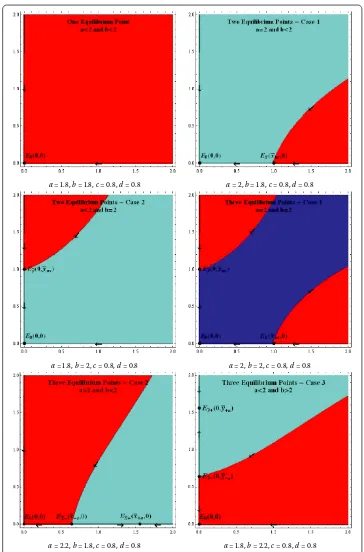
Theorem Assume that a< and b< .Then the zero equilibrium of()is globally asymptotically stable.
Proof It follows immediately from Theorem .
Theorem
attraction of the two equilibrium points are given as
whereWs(E)denotes the global stable manifold guaranteed by Theorem.
(b) Similarly,ifa< ,b= ,the basins of attraction of the equilibrium points are given as BE(, )
Proof We will present the proof of (a) since the proof of (b) uses analogous arguments. Lo-cal stability of the equilibrium points follows from Theorem . Furthermore, the existence
of the stable manifoldWs(E
¯
x) follows from Theorem . By immediate checking one can
see that ifx>x¯thenTn(x, )→Exasn→ ∞and ifx<x¯thenTn(x, )→Easn→
Another proof of this result follows from Theorem , which guarantees the existence
and uniqueness ofWs(E
¯
x) and the invariance of the regions below and aboveWs(Ex¯) and
Theorem , which guarantees that all solutions converge to an equilibrium point.
Theorem
(a) Ifa< ,b> ,then system()has three equilibrium points,E,E¯y+,E¯y–,where the first two are locally stable and the third is a saddle point.The basins of attraction of the three equilibrium points are given as
BE(, )
whereWs(E)denotes the global stable manifold guaranteed by Theorem.
attraction of three equilibrium points are given as
whereWs(E)denotes corresponding global stable manifold.
Proof We present the proof in case (a) only. The proof in case (b) is similar. Local stability of the equilibrium points follows from Theorem .
In view of Theorem all solutions converge to an equilibrium solution. Furthermore, all conditions of Theorem are satisfied, which guarantee the existence of the manifold Ws(E¯
y–), which is the graph of a continuous increasing function and such that both
re-gions, below and above it are invariant. In addition the basin of attraction ofEy¯–is exactly
Ws(E ¯
y–). Thus, both regions, below and aboveWs(Ey¯–) are invariant and contain exactly
one equilibrium point and all solutions there are convergent. Consequently the conclusion of the theorem follows.
Let us consider case (c). The existence and the properties of the manifoldsWs(E
¯
x) contains only one equilibrium point in view of Theorem all solutions that start
in those regions converge toE¯yandE¯x, respectively.
Now, let (x,y) be an arbitrary point betweenWs(Ey¯) andWs(Ex¯). First assume that
See Figure for visual illustration of Theorems -.
Theorem
(a) Ifa> ,b= ,then system()has four equilibrium points,E,E¯x+,E¯x–,E¯y,where the first two are locally asymptotically stable,the third is a saddle point and the fourth is non-hyperbolic of the stable type.The basins of attraction of the four equilibrium points are given as
a= .,b= .,c= .,d= . a= ,b= .,c= .,d= .
a= .,b= ,c= .,d= . a= ,b= ,c= .,d= .
a= .,b= .,c= .,d= . a= .,b= .,c= .,d= .
(b) Similarly,ifa= ,b> ,then system()has four equilibrium pointsE,Ey¯+,Ey¯–,Ex¯, where the first two are locally asymptotically stable,the third is a saddle point and the fourth one is non-hyperbolic of the stable type.The basins of attraction are given as
B(E) =
Proof We present the proof in case (a) only. The proof in case (b) is similar. Local stability of the equilibrium points follows from Theorem . The proof for the basin of attraction
B(Ey¯) is identical to the proof of the corresponding part of Theorem . Let (x,y) be
an arbitrary point belowWs(E
¯
is unique and represents the basin of attraction of the pointEx¯–.
Finally, let (x,y) be an arbitrary point betweenWs(E¯y) andWs(Ex¯–). First assume that
Theorem Assume that a> ,b> and that system()has five equilibrium points.
Three of these equilibrium points are locally asymptotically stable,E,Ex¯+,E¯y+,and two are saddle points,Ex¯–,E¯y–.
The basins of attraction of the equilibrium points are given as
B(E) =
The basins of attraction of the saddle equilibrium points E are the corresponding stable manifoldsWs(E).
Proof Local stability of the equilibrium points follows from Theorem . Furthermore, the existence of the stable manifoldsWs(E¯
x–) andWs(E¯y–) with the mentioned properties
fol-lows in the same way as in Theorem . The three regionsB(E),B(Ex¯+),B(Ey¯+) are
invari-ant by Theorem and in view of Theorem every solution converges to an equilibrium point. Since the equilibrium pointsE,Ex¯+,E¯y+ are locally asymptotically stable andE¯x–,
Theorem Assume that a> ,b> and that system()has six equilibrium points.Three of these equilibrium points are locally asymptotically stable,E,E¯x+,E¯y+,two are saddle points,E¯x–,Ey¯–,and one interior point,Enu,is non-hyperbolic of the unstable type.There exist two invariant curvesCuandCl emanating from Enuwhich are graphs of continuous non-decreasing functions such thatCuis aboveCl.
The basins of attraction of the equilibrium points are given as
B(E) =
Proof Local stability of the equilibrium points follows from Theorem . Furthermore, the existence of the stable manifoldsWs(E¯
x–) andWs(E¯y–) with the mentioned properties
fol-lows from Theorem . The regionB(E) is invariant by Theorem and in view of
The-orem every solution which starts in that region converges to E. The existence and
the properties of the curvesCl andCufollow from Corollary . Thus the regionsB(Ex¯+)
andB(Ey¯+) are both invariant and so by Theorem every solution which starts in those
regions converges toE¯x+ andE¯y+, respectively, since these equilibrium points are locally
asymptotically stable. Finally, the setB(Enu) is invariant by Theorem and by Theorem
every solution which starts in that region converges toEnu.
Conjecture Based on our numerical experiments we believe thatCl=Cuin Theorem holds.
Theorem Assume that a> ,b> and that system()has seven equilibrium points.
Three of these equilibrium points are locally asymptotically stable,E,E¯x+,Ey¯+,three are saddle points,E¯x–,E¯y–,ENWor ESE,and one is a repeller,ESW.
The basins of attraction of the equilibrium points are given as
B(E) =
The basins of attraction of the saddle equilibrium points E are the corresponding stable manifoldsWs(E).
Proof Local stability of all equilibrium pointsE,Ex±¯ ,E¯y±follows from Theorem .
Three regionsB(E),B(Ex¯+),B(Ey¯+) are invariant by Theorem and in view of
Theo-rem every solution converges to an equilibrium. Since the equilibrium pointsE,Ex¯+,
E¯y+ are locally asymptotically stable andE¯x–,E¯y–,ENWorESEare saddle points, the result
follows.
a= .,b= ,c= .,d= . a= ,b= .,c= .,d= .
a= .,b= .,c= .,d= . a= ,b= ,c= ,d=
a= .,b= .,c= .,d= . a= .,b= .,c= .,d= .
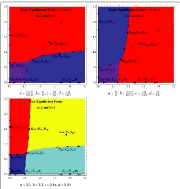
Theorem Assume that a> ,b> and that system()has eight equilibrium points.
Three of these equilibrium points are locally asymptotically stable,E,E¯x+,Ey¯+,three are saddle points,E¯x–,E¯y–,ENWor ESE,one is a repeller,ESW,and one is non-hyperbolic of the stable type Ens.
The basins of attraction of the equilibrium points are given as
B(E) =
The basins of attraction of the saddle equilibrium points E are the corresponding stable manifoldsWs(E).
The same result holds if ESWis replaced with ENE.
Proof Local stability of the equilibrium points follows from Theorem . The existence and
the properties of four manifoldsWs(E
¯
x–),Ws(Ey¯–),Ws(ESE),Ws(Ens) follow from
Theo-rem .
The four regionsB(E),B(Ex¯+),B(Ey¯+),B(Ens) are invariant by Theorem and in view
of Theorem every solution converges to an equilibrium point. Since the equilibrium pointsE,Ex¯+,Ey¯+ are locally asymptotically stable,Ensis non-hyperbolic of stable type
andEx¯–,Ey¯–,ESEare saddle points, the result follows.
Theorem Assume that a> ,b> and that system()has nine equilibrium points.
Four of these equilibrium points are locally asymptotically stable,E,Ex¯+,Ey¯+,ENE,four are saddle points,Ex¯–,E¯y–,ENW,ESE,and one is a repeller,ESW.
The basins of attraction of the equilibrium points are given as
B(E) =
The basins of attraction of the saddle equilibrium points E are the corresponding stable manifoldsWs(E).
Proof Local stability of the equilibrium points follows from Theorem . The existence
and the properties of four manifoldsWs(E
¯
x–),Ws(E¯y–),Ws(ESE),Ws(ENW) follow from
Theorem .
The four regionsB(E),B(Ex¯+),B(E¯y+),B(ENE) are invariant by Theorem and in view
of Theorem every solution converges to an equilibrium point. Since the equilibrium pointsE,E¯x+,E¯y+,ENEare locally asymptotically stable andE¯x–,E¯y–,ENW, andESEare
saddle points, the result follows.
a=, ,,b=
,c=
,d=
, a= ,b=
, ,,c=
,,d=
a= .,b= .,c= .,d= .
Figure 6 Global stability and basins of attraction of system (6) in cases of eight and nine equilibrium points.
Competing interests
The authors declare that they have no competing interests.
Authors’ contributions
Each of the authors, AB and MRSK, contributed to each part of this work equally and read and approved the final version of the manuscript.
Acknowledgements
The authors are grateful to two anonymous referees for a number of helpful and constructive suggestions.
Received: 27 August 2014 Accepted: 17 November 2014 Published:03 Dec 2014
References
1. Agarwal, RP: Difference Equations and Inequalities: Theory, Methods, and Applications, 2nd edn. Monographs and Textbooks in Pure and Applied Mathematics, vol. 228. Dekker, New York (2000)
2. Kulenovi´c, MRS, Ladas, G: Dynamics of Second Order Rational Difference Equations. Chapman & Hall/CRC, Boca Raton (2001)
3. Kulenovi´c, MRS, Merino, O: Discrete Dynamical Systems and Difference Equations with Mathematica. Chapman & Hall/CRC, Boca Raton (2002)
4. Thieme, HR: Mathematics in Population Biology. Princeton Series in Theoretical and Computational Biology. Princeton University Press, Princeton (2003)
5. Allen, LJS: An Introduction to Mathematical Biology. Prentice Hall, New York (2006)
6. Cushing, JM: The Allee effect in age-structured population dynamics. In: Hallam, TG, Gross, LJ, Levin, SA (eds.) Mathematical Ecology, pp. 479-505. World Scientific, Singapore (1988)
8. Thomson, GG: A proposal for a threshold stock size and maximum fishing mortality rate. In: Smith, SJ, Hunt, JJ, Rivard, D (eds.) Risk Evaluation and Biological Reference Points for Fisheries Management. Canad. Spec. Publ. Fish. Aquat. Sci., vol. 120, pp. 303-320 (1993)
9. Basu, S, Merino, O: On the global behavior of solutions to a planar system of difference equations. Commun. Appl. Nonlinear Anal.16, 89-101 (2009)
10. Brett, A, Kulenovi´c, MRS: Basins of attraction of equilibrium points of monotone difference equations. Sarajevo J. Math.5(18)(2), 211-233 (2009)
11. Brett, A, Kulenovi´c, MRS: Basins of attraction for two species competitive model with quadratic terms and the singular Allee effect. Discrete Dyn. Nat. Soc.2014, Article ID 847360 (2014)
12. Burgi´c, D, Kalabuši´c, S, Kulenovi´c, MRS: Nonhyperbolic dynamics for competitive systems in the plane and global period-doubling bifurcations. Adv. Dyn. Syst. Appl.3, 229-249 (2008)
13. Kulenovi´c, MRS, Merino, O: Invariant manifolds for competitive discrete systems in the plane. Int. J. Bifurc. Chaos20, 2471-2486 (2010)
14. Kulenovi´c, MRS, Nurkanovi´c, M: Asymptotic behavior of two dimensional linear fractional system of difference equations. Rad. Mat.11, 59-78 (2002)
15. Kulenovi´c, MRS, Nurkanovi´c, M: Asymptotic behavior of a competitive system of linear fractional difference equations. Adv. Differ. Equ.2006, Article ID 19756 (2006)
16. Livadiotis, G, Elaydi, S: General Allee effect in two-species population biology. J. Biol. Dyn.6, 959-973 (2012) 17. Livadiotis, G, Assas, L, Elaydi, S, Kwessi, E, Ribble, D: Competition models with Allee effects. J. Differ. Equ. Appl.20,
1127-1151 (2014)
18. Chow, Y, Jang, S: Multiple attractors in a Leslie-Gower competition system with Allee effects. J. Differ. Equ. Appl.20, 169-187 (2014)
19. Cushing, JM, Levarge, S, Chitnis, N, Henson, SM: Some discrete competition models and the competitive exclusion principle. J. Differ. Equ. Appl.10, 1139-1152 (2004)
20. Clark, D, Kulenovi´c, MRS, Selgrade, JF: Global asymptotic behavior of a two-dimensional difference equation modelling competition. Nonlinear Anal. TMA52, 1765-1776 (2003)
21. Franke, JE, Yakubu, A-A: Mutual exclusion versus coexistence for discrete competitive systems. J. Math. Biol.30, 161-168 (1991)
22. Franke, JE, Yakubu, A-A: Global attractors in competitive systems. Nonlinear Anal. TMA16, 111-129 (1991)
23. Franke, JE, Yakubu, A-A: Geometry of exclusion principles in discrete systems. J. Math. Anal. Appl.168, 385-400 (1992) 24. Hassell, MP, Comins, HN: Discrete time models for two-species competition. Theor. Popul. Biol.9, 202-221 (1976) 25. Hirsch, M, Smith, H: Monotone dynamical systems. In: Handbook of Differential Equations: Ordinary Differential
Equations, vol. II, pp. 239-357. Elsevier, Amsterdam (2005)
26. Hirsch, M, Smith, HL: Monotone maps: a review. J. Differ. Equ. Appl.11, 379-398 (2005)
27. Jiang, H, Rogers, TD: The discrete dynamics of symmetric competition in the plane. J. Math. Biol.25, 573-596 (1987) 28. Krawcewicz, W, Rogers, TD: Perfect harmony: the discrete dynamics of cooperation. J. Math. Biol.28, 383-410 (1990) 29. Kulenovi´c, MRS, Merino, O: Competitive-exclusion versus competitive-coexistence for systems in the plane. Discrete
Contin. Dyn. Syst., Ser. B6, 1141-1156 (2006)
30. Kulenovi´c, MRS, Merino, O: Global bifurcation for competitive systems in the plane. Discrete Contin. Dyn. Syst., Ser. B
12, 133-149 (2009)
31. Kulenovi´c, MRS, Nurkanovi´c, M: Global asymptotic behavior of a two dimensional system of difference equations modelling cooperation. J. Differ. Equ. Appl.9, 149-159 (2003)
32. Kulenovi´c, MRS, Nurkanovi´c, M: Asymptotic behavior of a linear fractional system of difference equations. J. Inequal. Appl.2005, 127-144 (2005)
33. May, RM: Stability and Complexity in Model Ecosystems. Princeton University Press, Princeton (2001)
34. Smith, HL: Periodic competitive differential equations and the discrete dynamics of competitive maps. J. Differ. Equ.
64, 165-194 (1986)
35. Smith, HL: Planar competitive and cooperative difference equations. J. Differ. Equ. Appl.3, 335-357 (1998) 36. Yakubu, A-A: The effect of planting and harvesting on endangered species in discrete competitive systems. Math.
Biosci.126, 1-20 (1995)
37. Yakubu, A-A: A discrete competitive system with planting. J. Differ. Equ. Appl.4, 213-214 (1998)
38. de Mottoni, P, Schiaffino, A: Competition systems with periodic coefficients: a geometric approach. J. Math. Biol.11, 319-335 (1981)
39. Smith, HL: Periodic solutions of periodic competitive and cooperative systems. SIAM J. Math. Anal.17, 1289-1318 (1986)
40. Hess, P: Periodic-Parabolic Boundary Value Problems and Positivity. Pitman Research Notes in Mathematics Series, vol. 247. Longman, Harlow (1991)
41. Camouzis, E, Kulenovi´c, MRS, Merino, O, Ladas, G: Rational systems in the plane. J. Differ. Equ. Appl.15, 303-323 (2009) 42. Kulenovi´c, MRS, Merino, O: Invariant curves of planar competitive and cooperative maps (to appear)
43. Clark, D, Kulenovi´c, MRS: On a coupled system of rational difference equations. Comput. Math. Appl.43, 849-867 (2002)
44. Yang, L, Hou, X, Zeng, Z: Complete discrimination system for polynomials. Sci. China Ser. E39(6), 628-646 (1996) 10.1186/1687-1847-2014-307