R E S E A R C H
Open Access
High-accuracy quasi-variable mesh
method for the system of 1D quasi-linear
parabolic partial differential equations based
on off-step spline in compression
approximations
RK Mohanty
1*and Sachin Sharma
2*Correspondence:
1Department of Applied
Mathematics, South Asian University, Akbar Bhawan, Chanakyapuri, New Delhi 110021, India
Full list of author information is available at the end of the article
Abstract
In this article, we propose a new two-level implicit method of accuracy two in time and three in space based on spline in compression approximations using two off-step points and a central point on a quasi-variable mesh for the numerical solution of the system of 1D quasi-linear parabolic partial differential equations. The new method is derived directly from the continuity condition of the first-order derivative of the spline function. The stability analysis for a model problem is discussed. The method is directly applicable to problems in polar systems. To demonstrate the strength and utility of the proposed method, we solve the generalized Burgers-Fisher equation, generalized Burgers-Huxley equation, coupled Burgers-equations and heat equation in polar coordinates. We demonstrate that the proposed method enables us to obtain high accurate solution for high Reynolds number.
MSC: 65M06; 65M12; 65M22; 65Y20
Keywords: quasi-linear parabolic equations; quasi-variable mesh; spline in compression; generalized Burgers-Fisher equations; coupled Burgers equation; Newton’s iterative method
1 Introduction
We consider the one-space dimensional quasi-linear parabolic partial differential equation (PDE) of the form
uxx=f(x,t,u,ux,ut), <x< ,t> . (.)
The initial and boundary conditions are given by
u(x, ) =u(x), ≤x≤, (.)
u(,t) =g(t), u(,t) =g(t), t> , (.)
where we assume that the functionsf,u(x),g(t) andg(t) are sufficiently smooth and
their required higher-order derivatives exist.
The quasi-linear parabolic equation describes a wide class of physical phenomenon such as the interaction between reaction mechanism, convection, effects and diffusion transports. It is used in many fields such as chemistry, biology, metallurgy and engineer-ing. The one-dimensional viscous generalized Burgers-Fisher equation (GBFE) and gen-eralized Burgers-Huxley equation (GBHE) are famous examples of quasi-linear parabolic equations.
The GBFE is given by
εuxx=ut+αuδux+βu
uδ– , t> , (.)
whereα,βare real parameters,δis a positive integer and <ε≤. The GBHE is given by
εuxx=ut+αuδux+βuuδ– uδ–γ, t> , (.)
whereα,β≥,γ ∈(, ),δ> and <ε≤ are the parameters.
In both cases, equations describe the interaction between diffusion, convection and re-action.
The GBFE has wide applications in the fields such as gas dynamics, fluid mechanics, elasticity, heat conduction and plasma physics. The well-known equation (.) was first used by Fisher [] to describe the propagation of gene in a habitat. In his memory, it is generally referred as Fisher’s equation. Whenα= andδ= , equation (.) reduces to the classical Fisher equation. Kolmogorovet al. [] independently wrote down the same equation to describe the dynamic spread of a combustion front. This equation has been found in various contexts in which a perturbation spreads in an excitable medium.
The GBHE was investigated by Satsuma et al. [] in . Whenε= ,α = ,δ= , equation (.) reduces to the Huxley equation and describes nerve pulse propagation in nerve fibers and wall motion in liquid crystals. Forε= , β= , equation (.) reduces to the generalized Burgers equation, which describes the far field of wave propagation in nonlinear dissipative systems. Whenε= ,α= ,β= andδ= , equation (.) becomes the Fitz-Hugh-Nagumo (FHN) equation which is the reaction diffusion equation used in circuit theory and biology. When α= , β= andδ= , equation (.) turns into the Burgers-Huxley equation (BHE) and shows a prototype model for describing the interac-tion between diffusion transports, convecinterac-tion and reacinterac-tion mechanisms.
Higher-order finite difference methods on a uniform mesh for the solution of nonlinear parabolic equations were proposed by Jainet al. []. Mittal and Jiwari [] developed dif-ferential quadrature method for numerical solution of coupled viscous Burgers’ equations. Mohantyet al. [] used compact operator technique to solve coupled Burgers’ equations. In recent past, Talwaret al. [] proposed spline in compression method based on three full-step grid points for the solution of D quasi-linear parabolic equations and in those methods the consistency equation is only second-order accurate and the method is not directly applicable to singular problems, which is a main drawback of those methods. To the best of the authors’ knowledge, no numerical method of order two in time and three in space, directly obtained from the consistency condition, for the solution of parabolic equation (.) on a quasi-variable mesh has been discussed in the literature so far.
In this paper, using a central point and two off-step points inx-direction, we propose a new two-level implicit method of accuracy two in time and three in space, based on spline in compression approximations for the solution of differential equation (.). The proposed method is obtained directly from the consistency condition and is of order three in space. Difficulties were experienced in the past for the higher-order spline solution of parabolic equation in polar coordinates. The solution usually deteriorates in the vicinity of the singularity. A special technique is required to handle such problems, whereas the pro-posed method is directly applicable to solve singular problems without any modification, which is the main attraction of our work. Our paper is arranged as follows: In Section , we discuss the non-polynomial spline in compression function and its properties on a quasi-variable mesh. In Section , we give derivation of the method. In Section , we generalize the proposed method for the system of quasi-linear parabolic PDEs. Stability analysis for model problem is discussed and it is shown that the linear scheme is unconditionally sta-ble in Section . In this section, we also discuss the stability analysis for a fourth-order parabolic equation which is consistent with system of D quasi-linear parabolic PDEs. In Section , numerical results are presented for some benchmark problems with tabu-lar and graphical illustrations and compare the results with the results obtained by other researchers. Final remarks are given in Section .
2 Spline in compression approximations and its properties
For the approximate solution of the initial-boundary value problems (.)-(.), we dis-cretize the space interval [, ] as =x<x<· · ·<xN <xN+= , whereNis a positive
integer. The spline approximation consists of two off-step pointsxl±/and a central point xl,l= , , , . . . ,Nwith two end pointsxandxN+, wherehl=xl–xl–,l= , , . . . ,N+ ,
be the mesh size in x-direction andk=tj+ –tj> , j= , , , . . . be the mesh spacing
int-direction. Spatial grid points are defined byxl=x+li=hi,l= ()N+ , and the
time steps are given bytj=jk,j= ()J, whereJis a positive integer. The mesh ratio is denoted by σl= (hl+/hl) > ,l= ()N. The neighboring off-step points are defined as xl–/=xl–hl andxl+/=xl+σlhl,l= ()N. Forσl= , it reduces to the uniform mesh
case. LetUlj=u(xl,tj) be the exact solution value ofu(x,t) and is approximated byujl. For simplicity, we considerσl=σ(a constant= ),l= ()N. Forσ> orσ< , the mesh sizes
are either increasing or decreasing in order. Such a mesh is called a quasi-variable mesh. A non-polynomial spline function of degree which interpolateujlatjth level is given by
which satisfy the following conditions atjth time level:
Using the conditions described above with algebraic calculations, we obtain the coeffi-cients spline in compression function
Pj(x) =Ulj+M
On differentiating equations (.) and (.), we get
and
On equating the coefficients ofMjlin (.), we obtain the condition
αl+βl+βl+γl=
( +σ)
+O
μl. (.)
Since the term σh
obtain the consistency condition
Ulj+– ( +σ)Ulj+σUlj–=σh
Further, substituting the values of (.a)-(.d) in (.) and neglectingO(μ
l) terms, we
get
tan(μl/) =μl/. (.)
The above equation has an infinite number of roots, the smallest positive non-zero root being given byμl=μ= .. Whenw→, then (αl,βl,βl,γl)→(σ,σ,,), and
equation (.) reduces to a cubic spline relation. Further, from equations (.)-(.), we get
Pj(xl–/) =
Simplifying (.) and (.), we obtain
Pj(xl–/) =
Equations (.) and (.) are two important properties of non-polynomial spline in compression functionPj(x).
3 Derivation of the numerical method
For the derivation of the method, we simply follow the approaches given by Mohanty []. At the grid point (xl,tj), let us denote
Differentiating the differential equation (.) partially with respect to ‘t’ at the grid point (xl,tj), we obtain a relation
At the grid point (xl,tj), we can write the differential equation as
SinceMjlandMjl±/contain the first derivative terms, from the consistency condition (.), the non-polynomial spline in compression method for the parabolic equation (.) can be written as
¯
where ‘θ’ is a parameter to be determined.
With the help of the approximations (.)-(.), we can simplify the following approx-imations:
From the properties of spline function given by (.) and (.), we define the approxi-mations:
ˆ
Uxlj =U¯xlj +bhlM¯lj+/–M¯jl–/, (.)
ˆ
Utlj =U¯tlj +cU¯tlj+– ( +σ)U¯tlj +σU¯tlj–, (.)
where ‘a’, ‘b’ and ‘c’ are parameters to be determined.
With the help of the approximation (.), (.), (.), from (.) we obtain
ˆ
Equating the coefficient ofh
l to zero in equation (.), we obtainb= –
Similarly, simplifying (.) and (.), we obtain
ˆ
With the help of the approximations (.), (.)-(.), (.)-(.), (.)-(.), from (.)-(.), we obtain
Using the approximation (.)-(.), (.)-(.), from (.), we obtain
+k( +σ)
Uγ
j l
+h
l
+σ+ a( +σ)Uαlj
+h
l
+σ+ cσ( +σ)Uγlj
+Tˆlj. (.)
Now with the help of the consistency condition (.) and equation (.), and from (.), we obtain the local truncation error
ˆ
Tlj=–σh
l
( +σ)
–θ
kUγlj+ hl
+σ+ a( +σ)Uαjl
+h
l
+σ+ cσ( +σ)Uγlj
+Okhl +hl, σ= . (.)
The proposed non-polynomial spline in compression method (.) to be ofO(khl+hl),
the coefficients ofkhl andhl in (.) must be zero.
Thus we obtainθ=,a=–(–σ+σ),c=–(–σ(+σ+σσ)) and the local truncation error given by (.) reduces toTˆlj=O(kh
l+hl).
4 Method extended to a system of quasi-linear parabolic equations
We now extend our method to the system of quasi-linear parabolic PDEs of the form
∂u
∂x = F, (.)
where u = [u(),u(), . . . ,u(n)]T, F = [f(),f(), . . . ,f(n)]T,Tdenotes the transpose of the
ma-trix.
Throughout this section, we consider
f(i)=f(i)x,t,u(),u(), . . . ,u(n),u()x ,u()x , . . . ,u(xn),u()t ,u()t , . . . ,u(tn)
, i= ()n.
The initial and boundary conditions are given by
u(i)(x, ) =u(i)(x), ≤x≤, (.)
u(i)(,t) =g(i)(t), u(i)(,t) =g(i)(t), t> , (.)
where we assume that the functionsu(i)(x),g(i)(t),g(i)(t) are sufficiently smooth.
LetUl(i)jandu(li)jbe the exact and approximate solution of theith PDE of the system (.) at each grid point (xl,tj). At the grid point (xl,tj), we define the following approximations:
¯
tj=tj+k
, (.)
¯
Ul(i)j=
Ul(i)j++Ul(i)j, (.)
¯
Ul(+i)j=
Finally, let
ˆ
Ml(i)j=f(i)xl,¯tj,Uˆl()j,Uˆl()j, . . . ,Uˆl(n)j,Uˆxl()j,Uˆxl()j, . . . ,Uˆxl(n)j,Uˆtl()j,Uˆtl()j, . . . ,Uˆtl(n)j, (.)
ˆ
M(l±i)j/=f(i)xl±/,tj¯,U¯l±()/j ,U¯ ()j l±/, . . . ,U¯
(n)j l±/,Uˆ
()j xl±/,Uˆ
()j xl±/, . . . ,
ˆ
Uxl±(n)j/,U¯tl±()j/,U¯tl±()j/, . . . ,U¯tl±(n)j/. (.) Then at each grid point (xl,tj), each differential equation of the system (.) is discretized by
¯
Ul(+i)j– ( +σ)U¯l(i)j+σU¯l(–i)j
=σh
l
σMˆ
(i)j l+/+
( +σ)
Mˆ
(i)j l +Mˆ
(i)j l–/
+Tˆl(i)j, i= ()n, (.)
whereTˆl(i)j=O(kh
l +hl), providedσ= . 5 Application and stability analysis
Now let us consider the one-dimensional Burgers equation in polar coordinates
Re
urr+p
rur– p ru
=ut+uur+g(r,t), <r< ,t> , (.)
whereRe> denotes the Reynolds number. Forp= and , the above equation represents Burgers’ equation in cylindrical and spherical coordinates, respectively. It is the simplest model for the differential equations of fluid flow. It is used in fluid dynamics as a simplified model for turbulence, boundary layer behavior and shock wave formation. The viscous Burgers equation in polar coordinates is a useful test equation for investigating various numerical schemes, which are then applied to more complicated systems of partial differ-ential equations. It shows a structure roughly similar to that of Navier-Stokes equations due to the form of the nonlinear convection term and the occurrence of the viscosity term. So it can be considered as a simplified form of the one-space dimensional Navier-Stokes equation. If we suppress the variablesθ,zandθ,ϕfrom the Navier-Stokes equations of motion in cylindrical polar coordinates (r,θ,z,t) and spherical polar coordinates (r,θ,ϕ,t), respectively (see []), we obtain Burgers’ equation (.) in polar coordinates. The high-accuracy numerical solution of Burgers’ equation in polar coordinates plays an important role for viscous fluid flow. It has been experienced in the past that the high-accuracy nu-merical solution usually deteriorates in the vicinity of the singular point sayr= , whereas the proposed spline method is applicable to D nonlinear parabolic equations irrespective of coordinates, that is, the proposed spline method is directly applicable to solve equa-tion (.). We do not require any modificaequa-tion in the spline scheme unlike other methods discussed in [, ]. Thus the numerical schemes for problems in polar coordinates are of importance in this discussion.
Re-write equation (.) as
εurr=ut+Q(r)ur+uur+S(r)u+g(r,t), (.)
whereRe=ε–> represents a Reynolds number andQ(r) = –pε
r ,S(r) = pε
Replacing the variable ‘x’ by ‘r’ and applying the method (.) to the differential equation
in the solution region without any modification. We do not require any fictitious point to solve the singular problem.
For stability, we consider the -D linear parabolic equation with variable coefficients
νuxx=ut+D(x)ux+f(x,t), <x< ,t> , (.)
whereν> andDandf are sufficiently smooth functions. Applying the method (.) to the differential equation (.) on a uniform mesh (that is, whenhl+=hl=h), we obtain
the following scheme for the solution of the above differential equation:
νU¯lj+– U¯lj+U¯lj–=h
The approximations associated with (.)-(.) are already defined in Section . In order to discuss the stability, we require the following approximations:
¯
With the help of the approximations (.)-(.) and (.)-(.), neglecting higher-order terms, from (.), we obtain
νδxU¯lj=h
Multiplying (.) throughout byλ= (k/h) and neglecting the local truncation error term, we have
To study the stability of scheme (.), we apply the von Neumann linear stability anal-ysis. Letεjl=ξjeiηlbe the error at the grid point (xl,tj), whereξis a complex number andη
is a real number. Substitutingεjl=ξjeiηlinto the homogeneous part of the error equation
of (.), we obtain the amplification factorξas
For stability, it is required that|ξ|≤. Imposing this condition on (.), we get
scheme (.) is unconditionally stable.
Next, we consider the fourth-order parabolic equations
whereε> andf is sufficiently smooth function.
The initial values ofu,ut are prescribed att= and boundary values ofu,uxxare
pre-scribed atx= andx= . Since the grid lines are parallel to the coordinate axes and the values ofu,uxx are exactly known on the boundary, the values of successive tangential partial derivatives ofu,uxx, i.e., the values ofut,uxxt, . . . , are also known on the boundary
x= andx= . Similarly, the values ofux,uxx,utx, . . . are also known att= . Hence the values ofuxx(x, ) –ut(x, ),uxx(,t) –ut(,t) anduxx(,t) –ut(,t) are known exactly on the boundary.
Now, equation (.) can be re-written as
εuxx=ut+v, (.a)
εvxx=vt+f(x,t). (.b)
Applying the numerical method (.) to the above system of equations and neglecting local truncation errors, we obtain the following non-polynomial spline in compression schemes in coupled form:
εu¯jl+– u¯jl+u¯jl–=h
Neglecting the homogeneous part, the above system in matrix form may be written as
Assume that the matrix A is non-singular. Pre-multiplying both sides of (.) by A–,
we get
respectively. Hence the eigenvalues of A are given byξ= – sinψ+ λεsinψ, and the eigenvalues of B are given byη= – sinψ– λεsinψ.
Since A–and B commute with each other, the eigenvalues of A–Bare given by
ρ= – sin
ψ– λεsinψ
– sinψ+ λεsinψ. (.)
For stability, it is required that|ρ| ≤ for all values ofψ. Imposing this condition on (.) yields
–≤ – sin
ψ– λεsinψ
– sinψ+ λεsinψ ≤. (.)
Both inequalities of (.) are true for all values ofψ. Hence the scheme (.a)-(.b) is unconditionally stable.
6 Numerical illustrations
In this section, we have solved several benchmark problems using the proposed method based on spline in compression and compared the results with the results obtained by other researchers. The exact solutions are provided in each case. The right hand side ho-mogeneous functions, initial and boundary conditions are obtained using the exact so-lution as a test procedure. The linear equations are solved using a tri-diagonal solver, whereas nonlinear equations are solved using the Newton-Raphson method. While us-ing the Newton-Raphson method, we choose as the initial guess. All the computations are carried out using MATLAB codes.
From equation (.), we have obtained the valueμl=μl+= .. In order to
compute the proposed method (.), we have evaluated the values of
αl=
σ μ
l+
μl+
sinμl+
–cosμl+
, βl=
σ μ
l+
[ –μl+cotμl+],
βl=
μ
l
[ –μlcotμl] and γl=
μ
l
μl
sinμl
–cosμl
using the values ofμlandμl+.
The given interval [, ] is divided into (N+ ) parts with =x<x<· · ·<xN <xN+= ,
wherehl=xl–xl–,l= , , . . . ,N+ andσ=hl+/hl> ,l= , , . . . ,N.
We can write
=xN+–x= (xN+–xN) + (xN–xN–) +· · ·+ (x–x)
=hN++hN+· · ·+h=
σN+σN–+· · ·+σ+σh. (.)
Thus,
h= /
σ+σ+· · ·+σN. (.) Alternatively, (.) can be re-written as
h= ( –σ)/
By prescribing the total number of mesh points (N+ ), we can compute the value of
h from (.) or (.). This is the first mesh spacing on the left and remaining mesh is
determined byhl+=σhl,l= , , . . . ,N.
Example The one-dimensional GBFE is given by the following form:
εuxx=ut+αuδux+βuuδ– , a≤x≤b,t> , (.)
where the real valued functionu=u(x,t) is a sufficiently smooth function of the space and time variables; [a,b] = [, ], andα,βare real parameters andδis a positive integer.
The initial condition associated with differential equation (.) is given by
u(x, ) = γ
+
γ
tanh(ax)
δ
, a≤x≤b, (.)
and the boundary conditions associated with (.) are given by
u(a,t) = γ
+
γ tanh
a(a–at)
δ
, t≥, (.)
u(b,t) = γ
+
γ tanh
a(b–at)
δ
, t≥. (.)
The exact solution [] of (.) is given by
u(x,t) = γ
+
γ tanh
a(x–at)
δ
, t≥, (.)
where
ε= , a=
–αδ
( +δ), a= α ( +δ)+
β( +δ)
α .
This problem is solved withN= , ,k= . and mesh ratioσ= . by present method. The following cases have been discussed for different values of the parameters α,β,γ andδ, which are involved in equation (.).
Case.: We chooseα= .,β= ..
Case.(a): In this case, results are computed for different time levels andδ= , . The maximum absolute errors are tabulated forx= ., ., . in Tables -.
Case.(b): In this case, results are computed for different time levels andδ= , , . The maximum absolute errors are tabulated fort= , , , , in Table .
Case.: We considerα= ,β= ,N= . In this case, results are computed for differ-ent time levelst= ., ., ., ., . andδ= , , . The maximum absolute errors are tabulated in Tables -.
Table 1 Example 1: Case 1.1(a)(i): Maximum absolute errors atδ= 1
x t Method given in [23] Method given in [5] Proposed method (3.6)
0.1 0.001 1.11(–16) 5.55(–16) 5.55(–17)
0.005 9.43(–16) 1.77(–15) 7.77(–16)
0.010 4.21(–15) 2.55(–15) 3.13(–14)
0.5 0.001 1.11(–16) 3.88(–16) 1.66(–16)
0.005 4.44(–16) 2.60(–15) 1.38(–15)
0.010 1.66(–16) 4.99(–15) 8.16(–15)
0.9 0.001 0 1.05(–15) 5.55(–17)
0.005 1.99(–15) 3.44(–15) 0
0.010 5.05(–15) 5.16(–15) 4.44(–16)
Table 2 Example 1: Case 1.1 (a)(ii): Maximum absolute errors atδ= 4
x t Method given in [23] Method given in [5] Proposed method (3.6)
0.1 0.001 1.11(–16) 3.76(–14) 1.11(–16)
0.005 2.22(–16) 1.43(–13) 9.99(–16)
0.010 6.66(–16) 2.39(–13) 1.75(–16)
0.5 0.001 1.12(–16) 3.20(–14) 1.11(–16)
0.005 3.33(–16) 1.61(–13) 3.33(–16)
0.010 3.33(–16) 3.22(–13) 2.88(–15)
0.9 0.001 1.11(–16) 3.84(–14) 1.11(–16)
0.005 5.55(–16) 1.45(–13) 1.11(–16)
0.010 1.11(–15) 2.41(–13) 2.22(–16)
Table 3 Example 1: Case 1.1(b): Maximum absolute errors
t δ= 1 δ= 4 δ= 8
1.0 3.44(–15) 9.95(–14) 9.55(–13) 2.0 1.66(–15) 9.61(–14) 9.54(–13) 3.0 1.33(–15) 9.73(–14) 9.61(–13) 4.0 1.31(–15) 9.76(–14) 9.88(–13) 5.0 1.22(–15) 9.78(–14) 9.89(–13)
Table 4 Example 1: Case 1.2(a): Maximum absolute errors atδ= 1
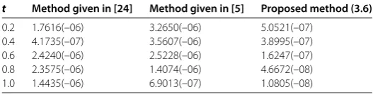
t Method given in [24] Method given in [5] Proposed method (3.6)
0.2 5.5574(–07) 3.5315(–07) 3.4453(–09) 0.4 9.0550(–07) 1.7573(–07) 2.9736(–09) 0.6 2.1880(–06) 1.2889(–07) 2.1401(–09) 0.8 2.9331(–06) 3.8543(–07) 1.5383(–09) 1.0 3.0145(–06) 6.1749(–07) 1.2262(–09)
Table 5 Example 1: Case 1.2(b): Maximum absolute errors atδ= 2
t Method given in [24] Method given in [5] Proposed method (3.6)
0.2 2.5610(–06) 7.9688(–07) 2.9321(–07) 0.4 4.2430(–06) 1.4540(–06) 3.9463(–07) 0.6 3.5684(–06) 1.8274(–06) 3.7075(–07) 0.8 1.4651(–06) 1.8775(–06) 2.7398(–07) 1.0 5.5423(–06) 1.6771(–06) 1.7040(–07)
Table 6 Example 1: Case 1.2(c): Maximum absolute errors atδ= 4
t Method given in [24] Method given in [5] Proposed method (3.6)
Table 7 Example 1: Case 1.3(a): Maximum absolute errors atδ= 1
x t Method given in [25] Method given in [5] Proposed method (3.6)
0.1 0.5 1.68(–11) 2.59(–12) 5.66(–13)
1.0 1.79(–11) 2.74(–12) 3.42(–13)
2.0 1.46(–11) 2.74(–12) 6.27(–13)
0.5 0.5 3.40(–12) 7.36(–13) 7.52(–14)
1.0 3.72(–12) 7.99(–13) 4.81(–14)
2.0 3.13(–12) 8.39(–13) 3.06(–14)
0.9 0.5 1.31(–11) 2.67(–12) 5.55(–17)
1.0 1.37(–11) 2.96(–12) 5.55(–17)
2.0 1.07(–11) 3.24(–12) 8.88(–16)
Table 8 Example 1: Case 1.3(b): Maximum absolute errors atδ= 2
x t Method given in [25] Method given in [5] Proposed method (3.6)
0.1 0.5 4.49(–11) 2.83(–11) 6.14(–12)
1.0 4.19(–11) 2.78(–11) 7.28(–12)
2.0 2.70(–11) 2.41(–11) 9.17(–12)
0.5 0.5 8.13(–12) 8.42(–12) 2.24(–13)
1.0 7.72(–12) 8.50(–12) 2.71(–13)
2.0 4.77(–12) 7.85(–12) 3.55(–13)
0.9 0.5 3.55(–11) 3.13(–11) 3.33(–16)
1.0 3.23(–11) 3.23(–11) 3.33(–16)
2.0 1.98(–11) 3.14(–11) 4.44(–16)
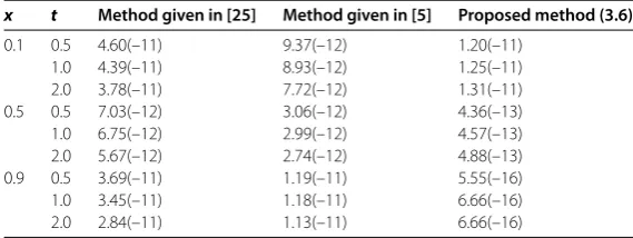
Table 9 Example 4: Case 1.3(c): Maximum absolute errors atδ= 8.
x t Method given in [25] Method given in [5] Proposed method (3.6)
0.1 0.5 4.60(–11) 9.37(–12) 1.20(–11)
1.0 4.39(–11) 8.93(–12) 1.25(–11)
2.0 3.78(–11) 7.72(–12) 1.31(–11)
0.5 0.5 7.03(–12) 3.06(–12) 4.36(–13)
1.0 6.75(–12) 2.99(–12) 4.57(–13)
2.0 5.67(–12) 2.74(–12) 4.88(–13)
0.9 0.5 3.69(–11) 1.19(–11) 5.55(–16)
1.0 3.45(–11) 1.18(–11) 6.66(–16)
2.0 2.84(–11) 1.13(–11) 6.66(–16)
Example Consider equation (.) withα= ,β= ,δ= initial and boundary condi-tions as given in Mittal and Jiwari [], namely
u(x, ) =x –x, <x< , (.a)
u(,t) =u(,t) = , t> . (.b)
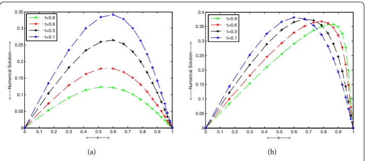
In this example, we have computed solutions forε= –and –att= ., ., ., .
with step sizek= . and mesh ratioσ= .. The computed numerical solutions as pre-sented in Figure (a)-(b) are consistent with the dynamics of the corresponding differential equations. Similar patterns have been presented in [, , ] also.
Example Consider equation (.) withα= ,δ= initial and boundary conditions as given in Zhaoet al. [], namely
(a) (b)
Figure 1 Example 2: Computed solutions for different time levels. (a)ε= 2–3,(b)ε= 2–6.
u(–,t) =u(,t) = , t> . (.b)
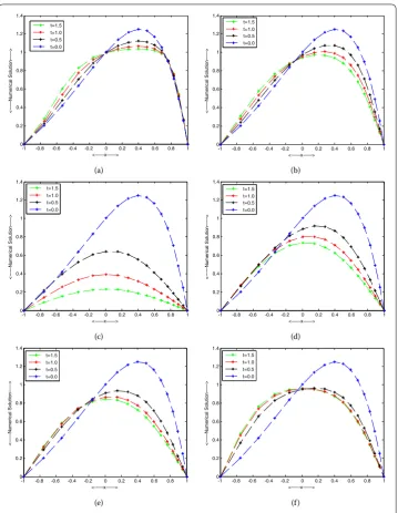
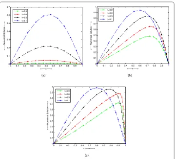
The computed numerical solutions for this example are presented in Figure (a)-(f ) for different value of the parameters. In our first computation, we compute the results for a fixed value of β and different value of εat different time levels. We take β = ,
t= ., ., ., . andε= ., ., ., respectively. The corresponding graphical so-lutions are presented in Figure (a)-(c). In our second computation, we compute the results for a fixed value ofεand different valued ofβat different time levels. We chooseε= .,
t= ., ., ., . andβ= ., ., ., respectively. The corresponding graphical results are presented in Figure (d)-(f ). The numerical solutions, as presented in Figure (a)-(f ), are consistent with those illustrated in [, ]. In Figure (a)-(c), the results exhibit that the numerical diffusion is dominated with the increasing diffusion coefficientε, whereas the reaction is gradually dominant with the increasing coefficientβas shown in Figure (d)-(f ). Thus, the computed and numerical solutions are in good agreement with the solution in the literature and the physical behavior of the differential equation.
Example The one-dimensional GBHE is given by the following form:
εuxx=ut+αuδux+βu
uδ– uδ–γ, a<x<b,t> , (.)
whereu=u(x,t) is sufficiently differentiable function, [a,b] = [, ],ε> is a small posi-tive parameter,αis real parameter,β≥,δ> ,γ ∈(, ) andγ= –( +γ). Whenα= ,
β= ,δ= and <ε, (.) is the well-known Burgers equation [], whereεis the coefficient of viscosity andRe=ε–> is the Reynolds Number.
The initial condition associated with differential equation (.) is given by
u(x, ) = γ
+
γ
tanh(ax) /δ
, a≤x≤b, (.)
and the boundary condition associated with the (.) are given by
u(a,t) = γ
+
γ tanh
a(a–at)
/δ
(a) (b)
(c) (d)
(e) (f )
Figure 2 Example 3: Computed solutions for different time levels. (a)ε= 0.005,β= 1.0,(b)ε= 0.05,
β= 1.0,(c)ε= 0.5,β= 1.0,(d)ε= 0.2,β= 1.5,(e)ε= 0.2,β= 2.5,(f)ε= 0.2,β= 5.0.
u(b,t) = γ
+
γ tanh
a(b–at)
/δ
, t≥, (.)
the exact solution [] of (.) is given by
u(x,t) = γ
+
γ tanh
a(x–at)
/δ
, t≥, (.)
where
ε= , a=
–αδ+δα+ β( +δ)
Table 10 Example 4: Case 4.1: Maximum absolute errors
x t δ= 1 δ= 2 δ= 4
0.1 0.1 6.7654(–17) 6.3838(–16) 6.4393(–15) 0.5 4.6404(–17) 4.8919(–16) 4.6352(–15) 0.9 4.7054(–17) 4.5797(–17) 4.9682(–15) 0.5 0.1 2.9816(–17) 3.4001(–16) 3.2752(–15) 0.5 4.2284(–17) 4.3716(–16) 4.2466(–15) 0.9 4.2609(–17) 4.2674(–16) 4.3854(–15) 0.9 0.1 1.0842(–19) 6.9389(–18) 2.7756(–17) 0.5 5.4210(–19) 6.9389(–18) 5.5511(–17) 0.9 5.4210(–19) 6.9389(–18) 5.5511(–17)
Table 11 Example 4: Case 4.2: Maximum absolute errors
x t β= 10 β= 100 β= 200
0.1 0.1 6.4393(–15) 6.6946(–14) 6.7590(–13) 0.5 2.6867(–14) 4.4409(–14) 2.6479(–14) 0.9 8.3267(–16) 8.8818(–15) 8.4044(–14) 0.5 0.1 5.2736(–15) 4.6241(–14) 4.5314(–13) 0.5 9.9809(–14) 7.0166(–14) 6.7590(–13) 0.9 7.0499(–15) 6.9666(–14) 7.0732(–13) 0.9 0.1 1.1102(–16) 7.7716(–16) 7.6050(–15) 0.5 2.6423(–14) 1.3878(–15) 1.4044(–14) 0.9 1.6653(–16) 1.3878(–15) 1.4044(–14)
a=
αγ ( +δ)+
( +δ–γ)(α+α+ β( +δ))
( +δ) .
The following cases have been discussed for different values of the parametersα,β,γ andδwhich are involved in Eq. (.).
Case.: In this case, we considerα= ,β= ,γ = . and mesh ratioσ = .. We have computed the numerical results for different time levels, namelyt= ., ., . with step sizek= . andδ= , , , respectively. Maximum absolute errors have been pre-sented forx= ., ., . in Table .
Case .: In this case, we consider α = , δ= , γ = – and mesh ratio σ = ..
We have computed the numerical results for fixed time level t = . with step size
k= . andβ= , , . Maximum absolute errors have been presented forx= ., ., ., ., . in Table .
Case .: In this case, we consider α = , β = , δ = . and mesh ratio σ = ..
We have computed the numerical results for fixed time level t = . with step size
k= . andγ = –, –, –. Maximum absolute errors have been presented for x= ., ., ., ., . in Table .
Case.: In this case, we considerα= ,β= and mesh ratioσ= .. We consider the initial and boundary conditions are given by
u(x, ) = εsin(πx)
+cos(πx), ≤x≤, (.)
u(,t) =u(,t) = , t≥. (.)
The exact solution [] is given by
u(x,t) =επexp(–επ
tsin(πx))
Table 12 Example 4: Case 4.3: Maximum absolute errors
x t γ= 10–2 γ= 10–3 γ= 10–4
0.1 0.1 1.1852(–13) 6.4193(–14) 7.1360(–15) 0.5 1.1358(–13) 3.6082(–14) 1.0680(–15) 0.9 1.0858(–13) 7.6883(–15) 8.4099(–15) 0.5 0.1 8.8096(–14) 5.2708(–14) 6.9000(–14) 0.5 8.4543(–14) 7.0194(–14) 6.9375(–14) 0.9 8.1157(–14) 6.8168(–14) 4.8003(–14) 0.9 0.1 2.3870(–15) 8.8818(–16) 1.4017(–15) 0.5 2.2760(–15) 1.3878(–15) 1.4017(–15) 0.9 2.2204(–15) 1.4155(–15) 7.7716(–16)
Table 13 Example 4: Case 4.4: Maximum absolute errorsα= 1,β= 0
N + 1 Proposed method (3.6) Method given in [4]
Re= 102 Re= 104 Re= 106 Re= 102 Re= 104 Re= 106
8 8.8258(–06) 1.9258(–09) 1.0430(–13) 4.1061(–04) 8.3710(–08) 8.4373(–12) 16 4.9239(–07) 9.7076(–11) 1.0463(–14) 1.1067(–04) 2.2489(–08) 2.2700(–12) 32 4.2004(–08) 7.3269(–12) 9.9642(–16) 2.7680(–05) 5.7437(–09) 5.7920(–13) 64 1.0396(–08) 1.2489(–12) 1.3421(–16) 6.9473(–06) 1.4564(–09) 1.4698(–13)
Results are computed for fixed time levelt= . and forδ= . Maximum absolute errors have been presented forRe=ε–= , , in Table .
Example We consider equation (.) with initial and boundary conditions are given in Mittal and Jiwari [], namely
u(x, ) =sin(πx), <x< , (.a)
u(,t) =u(,t) = , t> . (.b)
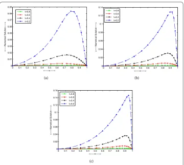
In our computation, we find solutions at different time levels for various decreasing values ofε. We taket= ., ., ., . with step sizek= . andε= –, –, –,
re-spectively. The computed solutions are interpreted graphically in Figure (a)-(c) forα= , β = ,δ= andγ = .. We notice that, for a fixed value of εas timet increases, the solutions curves fall to zero. Thus, the obtained solutions explain the nature of equation (.) faithfully in terms of diffusivity versus time. The approximate numerical solutions obtained by the present method exhibit correct physical behavior for several values ofε andt. Similar patterns have been depicted in [].
Example We consider equation (.) with initial and boundary conditions as given in Kaushik [], namely
u(x, ) = –cos(x), <x< , (.a)
u(,t) =u(,t) = , t> . (.b)
We computed numerical solutions for different time levels for various decreasing values ofε. We taket= ., ., ., . with step sizek= . andε= –, –, –, respectively.
(a) (b)
(c)
Figure 3 Example 5: Computed solutions for different time levels. (a)ε= 2–1,(b)ε= 2–4,(c)ε= 2–6.
in terms of diffusivity versus time. As the time increases, solution curves decreases to zero. For the decreasing value ofε, curves become steeper and propagate to the right which is the behavior of shocks waves. Similar patterns have been presented in [, ] also.
Example The coupled viscous nonlinear Burgers equation is given by the following
form:
ε∂
u
∂x =
∂u
∂t +αu
∂u
∂x+α
∂(uv)
∂x , a<x<b,t> , (.)
ε∂
v
∂x =
∂v
∂t+βv
∂v
∂x+β
∂(uv)
∂x , a<x<b,t> . (.)
Here <ε is the viscosity,Re=ε–> is the Reynolds number,α andβare real
constants,αandβare arbitrary constants depending on the system parameters []. The
coupled Burgers equations (.) and (.) represent a system of one-space dimensional quasi-linear parabolic equations with two unknown variablesuandv.
The initial condition associated with differential equations (.) and (.) is given by
(a) (b)
(c)
Figure 4 Example 6: Computed solutions for different time levels. (a)ε= 2–4,(b)ε= 2–6,(c)ε= 2–7.
and the boundary conditions associated with (.), (.) are given by
u(–π,t) =u(π,t) = , ≤t≤T, (.)
v(–π,t) =v(π,t) = , ≤t≤T. (.)
The values of parameters are given byα=β= – andα=β= . The exact solutions
of equations (.), (.) areu(x,t) =e–tsinxandv(x,t) =e–tsinx(see []).
In this example, we choose a uniform mesh (σ= ) to compute the numerical solutions for different values of the parametersε,α,α,βandβwith different values ofhandk.
In our first computation, we chooseε= ,α=β= –,α=β= ,h=π,k= . and
maximum absolute errors are computed at various time levels fromt= . to .. The corresponding results are tabulated in Table . In our second computation, the maximum absolute errors are computed att= . andt= . for a fixedλ= .
π,ε= ,α=β= –,
α=β= . Numerical results are presented in Table .
Example We consider the coupled Burgers equations (.), (.) with the following
initial and boundary conditions:
Table 14 Example 7: Maximum absolute error atε= 1,α1=β1= –2,α2=β2= 1,h= 2π/100,
k= 0.01
t Proposed method (4.28) Method discussed in [11]
u v u v
0.5 2.5045(–06) 2.5045(–06) 1.5168(–04) 1.5168(–04) 1.0 3.0373(–06) 3.0373(–06) 1.8397(–04) 1.8397(–04) 2.0 2.2330(–06) 2.2330(–06) 1.3525(–04) 1.3525(–04) 3.0 1.2296(–06) 1.2296(–06) 7.4601(–05) 7.4601(–05)
Table 15 Example 7: Maximum absolute errors,ε= 1,α1=β1= –2,α2=β2= 1,λ= 1.6/4π2
N + 1 Proposed method (4.28) Method given in [10] t = 1.0 t = 2.0 t = 1.0 t = 2.0
8 u 5.7826(–04) 4.2579(–05) 7.4756(–04) 6.1386(–04)
v 5.7826(–04) 4.2579(–05) 7.4756(–04) 6.1386(–04) 16 u 3.5478(–05) 2.6105(–07) 5.1124(–05) 3.8618(–05)
v 3.5478(–05) 2.6105(–07) 5.1124(–05) 3.8618(–05) 32 u 2.2070(–06) 1.6238(–06) 3.3516(–06) 2.4173(–06)
v 2.2070(–06) 1.6238(–06) 3.3516(–06) 2.4173(–06) 64 u 1.3777(–07) 1.0137(–07) 2.2035(–07) 1.5114(–07)
v 1.3777(–07) 1.0137(–07) 2.2035(–07) 1.5114(–07) 128 u 8.6048(–09) 6.3339(–09) 1.3837(–08) 9.3878(–09)
v 8.6048(–09) 6.3339(–09) 1.3837(–08) 9.3878(–09)
Table 16 Example 8: Maximum absolute errors att= 1,α1=β1= 2,α2=β2= –1,λ= 3.2
N + 1 Proposed method (4.28) Method given in [10]
Re= 100 Re= 200 Re= 250 Re= 100 Re= 200 Re= 250
8 u 6.3075(–06) 3.9152(–06) 3.2823(–06) 8.0563(–06) 4.3982(–06) 3.5838(–06)
v 6.3075(–06) 3.9152 (–06) 3.2837(–06) 8.0563(–06) 4.3982(–06) 3.5838(–06) 16 u 4.1145(–07) 2.4266(–07) 2.0268(–07) 5.0129(–07) 2.8249(–07) 2.2612(–07)
v 4.1145(–05) 2.4266(–07) 2.0268(–07) 5.0129(–07) 2.8249(–07) 2.2612(–07) 32 u 2.5696(–08) 1.5236(–08) 1.2647(–08) 3.1617(–08) 1.7629(–08) 1.4379(–08)
v 2.5696(–08) 1.5236(–08) 1.2647(–08) 3.1617(–08) 1.7629(–08) 1.4379(–08) 64 u 1.6133(–09) 9.5490(–10) 7.9187(–10) 1.9755(–09) 1.1015(–09) 8.9877(–10)
v 1.6133(–09) 9.5490(–10) 7.9187(–10) 1.9755(–09) 1.1015(–09) 8.9877(–10) 128 u 1.0082(–10) 5.9683(–11) 4.9531(–11) 1.2337(–10) 6.8803(–11) 5.6159(–11)
v 1.0082(–10) 5.9683(–11) 4.9531(–11) 1.2337(–10) 6.8803(–11) 5.6159(–11)
and
u(,t) =v(,t) =e–επt, ≤t≤T, (.)
u(,t) =v(,t) = –e–επt, ≤t≤T. (.)
In this example, we choose a uniform mesh size to compute the numerical solution for different parametersα=β= andα=β= –, the exact solutions of equations (.),
(.) areu(x,t) =e–επtcos(πx) andv(x,t) =e–επtcos(πx).
We computed the maximum absolute errors at time t= for a fixedλ= . and the
parametersα=β= ,α=β= – with the decreasing values ofhandk, and different
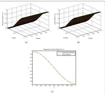
values ofRe=ε–. The numerical results are reported in Table . The graphs of numerical and exact solutions att= are plotted in Figure (a)-(c).
(a) (b)
(c)
Figure 5 Example 8: The graphs of numerical and exact solutions for the valuesα1=β1= 2,
α2=β2= –1,Re= 200 att= 1. (a)Numerical solution ofu=v,(b)Exact solution ofu=v,(c)Numerical and
exact solution forN+ 1 = 16.
Table 17 Example 9: Maximum absolute errors att= 1,k= 0.01
N + 1 p = 1 p = 2
Re= 10 Re= 100 Re= 10 Re= 100
50 1.6813(–06) 4.6778(–06) 1.5631(–06) 4.6698(–06) 60 1.4553(–06) 4.6745(–06) 1.3410(–06) 4.6676(–06) 70 1.2087(–06) 4.6677(–06) 1.1388(–06) 4.6634(–06) 80 9.1317(–07) 4.6789(–06) 8.5845(–07) 4.6621(–06) 90 6.1444(–07) 4.6794(–06) 5.4123(–07) 4.6623(–06)
t= for a fixedk= .,p= and and for various values ofRe=ε–. The corresponding
numerical results are reported in Table . The graphs of numerical and exact solutions at
t= are plotted in Figure .
7 Final remarks
In this article, we have presented a new two-level implicit method based on spline in compression approximations of accuracyO(khl+hl) for the numerical solution of
Figure 6 Example 9: The graph of numerical and exact solution atRe= 10,p= 1,N+ 1 = 50, k= 0.01.
convection-diffusion equation and fourth-order parabolic equation is presented. We have solved several benchmark problems using proposed method and it successfully provides highly accurate solutions in different settings of parameters. For different values of the parameters involved in GBFE, we have computed maximum absolute errors in Example and we observe that our method is giving more accurate results than the results obtained by [, –]. In Examples and , we have plotted the graphs (Figure (a)-(b) and Fig-ure (a)-(f )) at different time levels and for different values of parameters in GBFE, which exhibits that the numerical diffusion is dominated with the increasing diffusion coefficient ε, whereas the reaction is gradually dominant with the increasing coefficientβ. Similar patterns of graphs have been presented in [, –]. We have compared the computed numerical solutions with the exact solutions of GBHE in Example . Maximum absolute errors have been tabulated. The results obtained are quite good and competent with exact solution available in the literature. In Examples and , we have plotted the graphs (Fig-ure (a)-(c) and Fig(Fig-ure (a)-(c)) at different time levels and different values of parameters involved in GBHE which describes that solution curves decreases to zero as time increases and for small value ofε, solution curves behave like a shocks waves. We have computed maximum absolute errors for coupled viscous nonlinear Burgers’ equation in Examples and . On comparing the nature of computed solution with the computed solutions avail-able in [, ], we obtained better results by our scheme. Also we have plotted graphs (Figure (a)-(c)) of exact versus numerical solutiont= . In Example , we have solved singular parabolic partial differential equation in polar coordinates and obtained maxi-mum absolute errors for cylindrical and spherical case. Att= , we have plotted graph (Figure ) of numerical versus exact solution for Example . It can be observed that the approximate solution computed with our scheme and exact solutions are identical.
Acknowledgements
The authors thank the reviewers for their valuable comments and suggestions, which substantially improved the standard of the paper. This research work is supported by CSIR-SRF, Grant No: 09/045(1161)/2012-EMR-I.
Competing interests
The authors declare that they have no competing interest.
Authors’ contributions
All authors drafted the manuscript, and they read and approved the final version.
Author details
Publisher’s Note
Springer Nature remains neutral with regard to jurisdictional claims in published maps and institutional affiliations.
Received: 9 May 2017 Accepted: 10 July 2017 References
1. Fisher, RA: The wave of advance of advantageous genes. Annu. Eugen.7, 353-369 (1937)
2. Kolmogorov, AN, Petrovskii, IG, Piskunov, NS: A study of the equation of diffusion with increase in the quantity of matter, and its application to a biological problem. Bjul. Moskovskogo Gos. Univ.1(7), 1-26 (1937)
3. Satsuma, J, Ablowitz, M, Fuchssteiner, B, Kruskal, M: Topics in Soliton Theory and Exactly Solvable Nonlinear Equations. World Scientific, Singapore (1987)
4. Bratsos, AG: A fourth order improved numerical scheme for the generalized Burgers-Huxley equation. Am. J. Comput. Math.1, 152-158 (2011)
5. Mohammadi, R: Spline solution of the generalized Burgers’-Fisher equation. Appl. Anal.91(12), 2189-2215 (2011) 6. Zhang, R, Yu, X, Zhao, G: The local discontinuous Galerkin method for Burgers-Huxley and Burgers-Fisher equations.
Appl. Math. Comput.218, 8773-8778 (2012)
7. Macias-Diaz, JE: On an exact numerical simulation of solitary wave-solutions of the Burgers-Huxley equation through Cardano’s method. BIT Numer. Math.54, 763-776 (2014)
8. Mittal, RC, Tripathi, A: Numerical solutions of generalized Burgers-Fisher and generalized Burgers-Huxley equations using collocation of cubic B-splines. Int. J. Comput. Math.92(5), 1053-1077 (2015)
9. Mohanty, RK, Dai, W, Liu, D: Operator compact method of accuracy two in time and four in space for the solution of time independent Burgers-Huxley equation. Numer. Algorithms70, 591-605 (2015)
10. Jain, MK, Jain, RK, Mohanty, RK: High order difference methods for system of 1-D non-linear parabolic partial differential equations. Int. J. Comput. Math.37, 105-112 (1990)
11. Mittal, RC, Jiwari, R: Differential quadrature method for numerical solution of coupled viscous Burgers’ equations. Int. J. Comput. Methods Eng. Sci. Mech.13, 88-92 (2012)
12. Mohanty, RK, Dai, W, Han, F: Compact operator method of accuracy two in time and four in space for the numerical solution of coupled viscous Burgers’ equations. Appl. Math. Comput.256, 381-393 (2015)
13. Talwar, J, Mohanty, RK, Singh, S: A new spline in compression approximation for one space dimensional quasilinear parabolic equations on a variable mesh. Appl. Math. Comput.260, 82-96 (2015)
14. Mohanty, RK: An implicit high accuracy variable mesh scheme for 1D non-linear singular parabolic partial differential equations. Appl. Math. Comput.186, 219-229 (2007)
15. Mohanty, RK, Setia, N: A new high order compact off-step discretization for the system of 3D quasi-linear elliptic partial differential equations. Appl. Math. Model.37, 6870-6883 (2013)
16. Mohanty, RK, Jain, MK: High-accuracy cubic spline alternating group explicit methods for 1D quasi-linear parabolic equations. Int. J. Comput. Math.86, 1556-1571 (2009)
17. Mohanty, RK: A variable mesh C-SPLAGE method of accuracyO(k2h–1+kh+h3) for 1D nonlinear parabolic equations.
Appl. Math. Comput.213, 79-91 (2009)
18. Mittal, RC, Jiwari, R: Numerical study of Burgers-Huxley equation by differential quadrature method. Int. J. Appl. Math. Mech.5, 1-9 (2009)
19. Kaushik, A: Pointwise uniformly convergent numerical treatment for the non-stationary Burgers-Huxley using grid equidistribution. Int. J. Comput. Math.84(10), 1527-1546 (2007)
20. Zhao, T, Li, C, Zang, Z, Wu, Y: Chebyshev-Legendre pseudo-spectral method for generalized Burgers-Fisher equation. Appl. Math. Model.36(3), 1046-1056 (2012)
21. Burgers, JM: A mathematical model illustrating the theory of turbulence. Adv. Appl. Mech.1, 171-199 (1948) 22. Kaya, D: An explicit solution of coupled viscous Burgers’ equations by the decomposition method. Int. J. Math. Math.
Sci.27, 675-680 (2001)
23. Sari, M, Gürarslan, G, Zeytinoglu, A: High-order finite difference schemes for the solution of the generalized Burgers’-Fisher equation. Commun. Numer. Methods Eng.27(8), 1296-1308 (2011)
24. Zhu, C-G, Kang, W-S: Numerical solution of Burgers’-Fisher equation by cubic B-spline quasi-interpolation. Appl. Math. Comput.216, 2679-2686 (2010)