Retrieval of long-wave tsunami Green’s function from the cross-correlation of
continuous ocean waves excited by far-field random noise sources
on the basis of a first-order Born approximation
Tatsuhiko Saito1and Jun Kawahara2
1National Research Institute for Earth Science and Disaster Prevention, 3-1 Tennodai, Tsukuba, Ibaraki 305-0006, Japan 2Faculty of Science, Ibaraki University, 2-1-1 Bunkyo, Mito, Ibaraki 310-8512, Japan
(Received April 1, 2011; Revised August 29, 2011; Accepted August 31, 2011; Online published March 2, 2012)
We investigate the theoretical background for the retrieval of the tsunami Green’s function from the cross-correlation of continuous ocean waves. Considering that a tsunami is a long-wavelength ocean wave described by 2-D linear long-wave equations, and that the sea-bottom topography acts as a set of point-like scatterers, we use a first-order Born approximation in deriving the tsunami Green’s function having coda waves. The scattering pattern is non-isotropic and symmetrical with respect to the forward and backward directions. We indicate a retrieval process which shows that the derivative of the cross-correlation function of wavefields at two receivers with respect to the lag time gives the tsunami Green’s function when point noise sources generating continuous ocean waves are distributed far from, and surrounding, the two receivers. Note that this relation between the cross-correlation and the Green’s function is different from the case in which uncorrelated plane-wave incidence from all directions is assumed to be continuous ocean waves. The Green’s function retrieved from continuous ocean waves will be used as a reference to examine the validity of the Green’s function obtained by numerical simulations.
Key words:Tsunami, theory, interferometry.
1.
Introduction
The technique of seismic interferometry, whereby the seismic Green’s function between two points is extracted from the cross-correlation of ambient seismic noise, has re-ceived a great deal of attention from seismologists (e.g., Campillo and Paul, 2003). Using this technique, seismol-ogists can calculate the Green’s function, or estimate sub-surface structures, by analyzing ambient noise, without the need for natural or artificial earthquakes (e.g., Shapiroet al., 2005; Nishidaet al., 2009). For tsunami researchers, it is necessary to use the correct tsunami Green’s functions for tsunami source inversion analysis (e.g., Satake, 1989; Saito et al., 2010) or for simulating disastrous tsunamis generated by past, and anticipated future, huge earthquakes (e.g., Furumuraet al., 2011). The correct tsunami Green’s function should be obtainable by numerical simulation us-ing accurate and high-resolution bathymetry data. How-ever, we cannot always obtain the correct Green’s func-tion through numerical simulafunc-tions. For example, in the 2010 Maule, Chile, earthquake tsunami, there was a sig-nificant discrepancy (∼30 min) between the observed, and simulated, arrival times around Japan (Satakeet al., 2010). Therefore, it would be very useful if we are able to synthe-size the tsunami Green’s function from observed “ambient” ocean waves; in other words, if we can retrieve the tsunami
Copyright cThe Society of Geomagnetism and Earth, Planetary and Space Sci-ences (SGEPSS); The Seismological Society of Japan; The Volcanological Society of Japan; The Geodetic Society of Japan; The Japanese Society for Planetary Sci-ences; TERRAPUB.
doi:10.5047/eps.2011.08.020
Green’s function from the cross-correlation of continuous ocean waves observed by, for example, ocean-bottom pres-sure gauges. Therefore, we investigate the theoretical back-ground for the retrieval of the tsunami Green’s function from the cross-correlation of continuous ocean waves. This is the first attempt to demonstrate a retrieval process of the tsunami Green’s function which, in particular, includes coda waves. Considering that the tsunami has a long wave-length and the sea-bottom topography acts as a set of point-like scatterers, we use a first-order Born approximation. The framework of the present study follows Sato (2009), who dealt with the case of 3-D scalar waves with isotropic scattering. For the application to a tsunami, the present study extends the approach of Sato to the case of 2-D waves with special non-isotropic scattering.
2.
Tsunami Green’s Function in a Scattering
Medium: Single Scattering
We assume that ocean waves and tsunamis obey a 2-D linear long-wave equation (e.g., equation (2) in Saito and Furumura, 2009) inx-ycoordinates. The sea depth is rep-resented ash(x)=h0{1+ξ (x)}, whereh0is the average sea depth, andh0ξ (x)is the fluctuation from the average. The fluctuation is assumed to be small, |ξ (x)| 1. The wave equation for an ocean wave, or tsunami,η (x,t), for a noise sourceN(x,t), is then given as follows:
∂2
∂x2 +
∂2
∂y2 − 1 V2
0
∂2
∂t2
η (x,t)
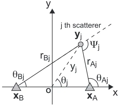
Fig. 1. Configuration of the two receivers, scatterers, and noise sources in x-y coordinates. The two receivers are located atxA andxB on thex-axis with a separation of 2h. The scatteres are localized within the region of sizeDaround the two receivers. The noise sources are randomly distributed in a circular shell of radius Rfar from the two receivers and scatterers (RD).
Fig. 2. Configuration of two pointsxAandxB, and a scatterer located at yj. When a source is located atxB, a wave radiated from the source propagates to the scattereryj and is scattered with an angle ofj. The scattered wave then arrives atxA.
+ξ (x)
∂2
η (x,t)
∂x2 +
∂2η (x,t)
∂y2
+
∂ξ (x)
∂x
∂η (x,t)
∂x +
∂ξ (x)
∂y
∂η (x,t)
∂y
=N(x,t) , (1)
whereV0=√g0h0, andg0is the gravitational acceleration. We solve Eq. (1) for a delta-function source term in the frequency domain, in order to obtain the Green’s function. The Green’s function Gˆ(x,x0, ω) for a source located at x=x0satisfies the following equation:
∂2
∂x2 +
∂2
∂y2 +k 2 0
ˆ
G(x,x0, ω)
+ξ (x)
∂2Gˆ(x,x0, ω)
∂x2 +
∂2Gˆ (x,x0, ω)
∂y2
+
∂ξ (x)
∂x
∂Gˆ(x,x0, ω)
∂x +
∂ξ (x)
∂y
∂Gˆ(x,x0, ω)
∂y
=δ (x−x0) , (2)
where the wavenumberk0 is given by k0 = ω/V0. The Green’s functionG0ˆ (x,x0, ω), for the constant sea depth h=h0, satisfies the following equation:
∂2
∂x2 +
∂2
∂y2 +k 2 0
ˆ
G0(x,x0, ω)=δ (x−x0) , (3)
and is given by,
ˆ
G0(x,x0, ω)
=−i
4 H
(1)
0 (k0|x−x0|)
≈−1
4
2 πk0|x−x0|
exp
i k0|x−x0| +iπ 4
for k0|x−x0| 1, (4)
whereH0(1) is the first Hankel function of order zero (e.g., Snieder, 2001). We assume that a receiver is located atxA = (h,0), and that a source is located atxB =(−h,0), on the
x-axis, with a separation distance of rA B = 2h (Fig. 1). Based on Sato (2009), the sea-bottom fluctuationξ (x)is
assumed to be represented asξ (x) =
N
j=1
εjd2δ x−y
j
,
whereεj is a scale factor adjusting the sea-bottom topog-raphy fluctuation and the spatial scaled is small compared with the tsunami wavelength. The sea-bottom fluctuation ξ (x)then acts as a set of point-like scatterers. The scatter-ers are located within a region of sizeDaroundxAandxB. The far-field scattered wave from the scatterers is theoreti-cally calculated by using a first-order Born approximation. We then obtain the Green’s function for Eq. (2) (Saito and Furumura, 2009) as follows:
ˆ
G(xA,xB, ω)
≈ ˆG0(xA,xB, ω)
+
N
j=1
ˆ
G0 xA,xj, ω
εjk20d2cosjGˆ0 xj,xB, ω
for kxA−xj, kxj−xB1. (5)
The anglej is the scattering angle for the jth scatterer located atyj and satisfies,
cosj = −cos θA j−θB j
, (6)
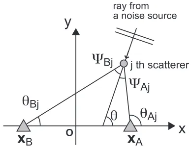
Fig. 3. Configuration of two receiversxA andxB, and a ray from a far-field noise source. The waves scattered at the jth scatterer arrive at the receiversxAandxBwith the scattering angles ofA j andB j, respectively.
3.
Cross-correlation Function of Waves in a
Scat-tering Medium Illuminated by Surrounding
Noise Sources
Noise sources with a spectrum Nˆ(x, ω) are distributed on a circle of radiusRwith a small widthR, whereRis much greater thanD(Fig. 1). The continuous ocean wave at locationxA, excited by the noise sources, is given in terms of polar coordinates(r, θ)by,
where θ is measured from the x-axis, and the sym-bol dθ indicates integration with respect to θ over a range of 2π. We imagine an ensemble of noise sources. When the locations of sources are not correlated, we may write the ensemble average of the noise spectra as
lim T→∞
ˆ
N(x, ω)∗Nˆ x, ωT =δ x−xSˆN(ω), where the * symbol represents a complex conjugate, T is the time window length, andSˆN(ω)is the power spectral den-sity function of stationary noise (Sato, 2009). Note that
ˆ
N(x, ω)∗ = ˆN(x,−ω)becauseN(x,t)is real. We define the cross-correlation function of continuous ocean waves observed atxA andxB over the ensemble of noise sources as
Substituting Eqs. (4) and (5) into Eq. (8), we calculate the integral with respect to θ. In this calculation, we use the approximation in the denominators√|xA−x| ≈
R as geometrical spreading factors, because the noise sources are distributed in the far field, R D. We also approximate the distance in the ex-ponent|xA−x| ≈R−hcosθ,|xB−x| ≈ R+hcosθ, and
yj−x ≈ R−yjcos θj−θ
, where yj = yj. These approximations are common to Sato (2009). The scattering anglesA j andB jare given byθA j−θandθ−θB j, re-spectively (Fig. 3). We then obtain the following equation for the integration with respect toθin Eq. (8):
where the second-order terms with respect to εj are neglected. For the calculation of the integral in the second term of Eq. (9), we use the relations
+sin θA j−θB j dθ sinθ expi k0rB jcosθ
=cos θA j−θB j 2πi J1 k0rB j
, (10)
where J1 is a Bessel function of the first order. Sim-ilarly, with the relation hcosθ − yjcos θ−θj lated. Then, using Eq. (4), we rewrite Eq. (9) as follows:
whereJ0andN0are Bessel and Neumann functions of order zero, respectively. Assuming a far fieldk0r 1 and using the approximation,Nn(k0r)≈Jn+1(k0r)(Abramowits and Stegun, 1972), we finally obtain,
Now, in order to compare Eq. (12) with the imaginary part of Eq. (5), we rewrite Eq. (5), by using Eq. (4), as
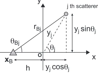
Fig. 4. Configuration of a receiverxBand thejth scatterer.
−J0 k0rA j
Finally, comparing Eqs. (12) and (13), we obtain the fol-lowing relation:
dθRGˆ(xA,x, ω)∗Gˆ(xB,x, ω)
≈ −1
k0ImGˆ(xA,xB, ω) , (14)
for the 2-D tsunami wave equation including the scattered waves from the point-like scatterers. This form of the 2-D tsunami equation is consistent with the counterpart for the 3-D case (e.g., equation (13) in Sato (2009)). Based on Eqs. (8) and (14), we obtain the relation in the time domain as follows: time domain and SN(τ) is the auto-correlation func-tion of the noise sources. In the calculation, we used
ˆ
G(xA,xB, ω)∗ = ˆG(xA,xB,−ω), becauseG(xA,xB,t)is real, andSˆN(−ω)= ˆSN(ω)becauseSN(−τ)=SN(τ).
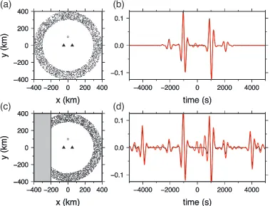
Fig. 5. (a) Configuration of the numerical simulations without land. The solid triangles, open circle, and dots denote receivers, a scatterer (island), and noise sources, respectively. (b) Waveform retrieved by the time derivative of the cross-correlation function (red) and the synthetic waveforms of the Green’s functions between the two stations (black) for the configuration of Fig. 5(a). (c) Configuration of the numerical simulations with land (shaded), inside which no noise sources exist. The locations of the receivers and the scatterer are unchanged from Fig. 5(a). (d) Waveform retrieved by the time derivative of the cross-correlation function (red) and the synthetic waveforms of the Green’s functions between the two stations (black) for the configuration of Fig. 5(d).
Equation (16) indicates the relation between the spatial cor-relation of continuous ocean waves and the tsunami Green’s function. The derivative of the cross-correlation function for the two receivers with respect to lag time gives the Green’s function.
Equation (16) for the 2-D tsunami is consistent with the counterpart for the 3-D scalar wave (e.g. Rouxet al., 2005; Sato, 2009). Note, however, that this form is different from that derived by Nakahara (2006) for 2-D scalar waves, in which the Hilbert transform of the cross-correlation func-tion gives the Green’s funcfunc-tion. The difference comes from the assumption of the noise sources. The present study sumes point noise sources, whereas Nakahara (2006) as-sumes uncorrelated plane-wave incidence as a noise wave-field. In 2-D space, a cylindrical wave impulsively radiated from a point source exhibits waveform broadening with a lapse time even in homogeneous media. By contrast, a plane wave maintains its initial shape during the propaga-tion. This causes the difference between the results obtained in the present study and those of Nakahara (2006), in which the broadening nature of the Green’s function is recovered by Hilbert-transforming the cross-correlation function.
4.
Numerical Examples
In order to validate the theoretical results of the present study, we performed numerical simulations based on the boundary integral method of Yomogida and Benites (1995), which was originally developed for simulating SH wave
scattering in 2-D elastic media with cavities. We herein apply this method to tsunami scattering. This is justified by the fact that the 2-D wave equation of a tsunami (Eq. (1)), and that ofSHwaves in an elastic media of constant density are mathematically equivalent. In this relationship between the tsunami and theSHwaves, a cavity in the elastic media corresponds to an island (a small area with zero sea depth). We take two receivers with a separation distance of 100 km, and one circular island with a radius of 10 km as a point-like scatterer, which are surrounded by 3,000 noise sources (Fig. 5(a)). Here, V0 = 0.1 km/s, R = 300 km, andR =100 km, and the distance between the scatterer and either receiver is 112 km. Each noise source radiates a Ricker wavelet with a dominant frequency of 0.003 Hz and a corresponding wavelength of 33 km, which is larger than the size of the scatterer. We numerically simulated the wave propagation from the noise sources and synthe-sized the wavefields at the two receivers. Figure 5(b) shows the time derivative of the cross-correlation function of these wavefields (corresponding to the left-hand side of Eq. (15)). We also synthesized the Green’s function between the two receivers (convolved with the auto-correlation function of the noise sources corresponding to the right-hand side of Eq. (15)), which is also shown in the figure. The agreement between the waveforms is confirmed to be excellent.
is 150 km. Although the number of noise sources is un-changed, there are no noise sources in the land. The tsunami reflected from the coast is recognized at±4,000 s in Fig. 5(d). Compared with the case of Fig. 5(b), the wave-form retrieved from the cross-correlation function partly disagrees with the synthesized Green’s function. In partic-ular, the amplitude with respect to the time axis is signif-icantly asymmetric in the Green’s function retrieved from the cross-correlation function, because of the uneven distri-bution of the noise sources in space. Nevertheless, the ar-rival times of the maximum-amplitude wave, the scattered wave, and the wave reflected from the land in the Green’s function retrieved from the cross-correlation function ex-plain well these arrival times for the synthesized Green function. This indicates that the retrieved Green’s function can be used as a reference in examining the validity of the travel time as calculated by numerical tsunami simulations.
5.
Concluding Remarks
The present paper describes a retrieval process for the 2-D tsunami Green’s function from the cross-correlation of continuous ocean waves based on a first-order Born ap-proximation. Equation (16) indicates that the derivative of the cross-correlation function for two receivers with respect to lag time gives the tsunami Green’s function including coda waves. Furthermore, we have presented numerical examples of the Green’s function retrieved from the cross-correlation function of the continuous waves to confirm the validity of the obtained results.
We herein assumed single scattering for the coda ex-citation. On the other hand, Margerin and Sato (2011) demonstrated the effects of a multiple scattering process in the retrieval of the 3-D scalar-wave Green’s function us-ing Feynman diagrams. Some studies have also taken the higher-order perturbation of waves into consideration for the retrieval process (Sanchez-Sesmaet al., 2006; Snieder et al., 2008; Wapenaar et al., 2010). A general theory of Green’s function retrieval for linear partial differential equations was recently presented by Fleuryet al.(2010). Such general theories, which are not (or, at least, not strongly) restricted by the approximation conditions, are obviously important. On the other hand, the simplicity of analyzing specific situations, such as tsunami propagation with single scattering, as considered in the present study, may also be useful. For example, such an analysis would be helpful in interpreting the numerical simulation results, or practical analyses, of observed tsunami records. For the case of tsunami propagation, since accurate high-resolution bathymetric data is available, it would be interesting to sim-ulate the retrieval of the tsunami Green’s function using ac-tual bathymetry data. The results reported herein will be helpful in interpreting the features of actual records and the retrieved Green’s functions.
Acknowledgments. The authors would like to thank K. Yomogida for allowing the use of his computer code for the bound-ary integral simulations. We would also like to thank H. Sato
and H. Nakahara for their useful discussions and advice. The manuscript was greatly improved by the careful reading and com-ments provided by T. Hara and the two anonymous reviewers.
References
Abramowits, M. and I. A. Stegun,Handbook of Mathematical Functions, Dover, Mineola, N.Y., 1972.
Campillo, M. and A. Paul, Long range correlations in the seismic coda,
Science,299, 547–549, 2003.
Fleury, C., R. Snieder, and K. Larner, General representation theorem for perturbed media and application to Green’s function retrieval for scat-tering problems,Geophys. J. Int.,183, 1648–1662, doi:10.1111/j.1365-246X.2010.04825.x, 2010.
Furumura, T., K. Imai, and T. Maeda, A revised tsunami source model for the 1707 Hoei earthquake and simulation of tsunami inundation of Ryu-jin Lake, Kyushu, Japan,J. Geophys. Res., doi:10.1029/2010JB007918, 2011.
Margerin, L. and H. Sato, Reconstruction of multiply-scattered ar-rivals from the cross-correlation of waves excited by random noise sources in a heterogeneous dissipative medium, Wave Motion, doi:10.1016/j.wavemoti.2010.10.001, 2011.
Nakahara, H., A systematic study of theoretical relations between spatial correlation and Green’s function in one-, two- and three-dimensional random scalar wavefields, Geophys. J. Int., 167, 1097– 1105, doi:10.1111/j.1365-246X.2006.03170.x, 2006.
Nishida, K., J. P. Montagner, and H. Kawakatsu, Global surface wave tomography using seismic hum,Science,326(5949), 112, 2009. Roux, P., K. G. Sabra, W. A. Kuperman, and A. Roux, Ambient noise cross
correlation in free space: Theoretical approach,J. Acoust. Soc. Am.,117, 79–84, 2005.
Saito, T. and T. Furumura, Scattering of linear long-wave tsunamis due to randomly fluctuating sea-bottom topography: Coda excitation and scat-tering attenuation,Geophys. J. Int.,177, 958–965, doi:10.1111/j.1365-246X.2009.03988.x, 2009.
Saito, T., K. Satake, and T. Furumura, Tsunami waveform inversion includ-ing dispersive waves: The 2004 earthquake off Kii Peninsula, Japan,J. Geophys. Res.,115, B06303, doi:10.1029/2009JB006884, 2010. Sanchez-Sesma, F. J., J. A. Perez-Ruiz, M. Campillo, and F. Luzon,
Elastodynamic 2D Green function retrieval from cross-correlation: Canonical inclusion problem, Geophys. Res. Lett., 33, L13305, doi:10.1029/2006GL026454, 2006.
Satake, K., Inversion of tsunami waveforms for the estimation of heteroge-neous fault motion of large submarine earthquakes: The 1968 Tokachi-oki and 1983 Japan Sea earthquakes,J. Geophys. Res.,94, 5627–5636, doi:10.1029/JB094iB05p05627, 1989.
Satake, K., S. Sakai, T. Kanazawa, Y. Fujii, T. Saito, and T. Ozaki, The February 2010 Chilean tsunami recorded on bottom pressure gauges, MIS050-P05, Japan Geoscience Union Meeting 2010, 2010.
Sato, H., Retrieval of Green’s function having coda from the cross-correlation function in a scattering medium illuminated by surrounding noise sources on the basis of the first order Born approximation, Geo-phys. J. Int., 179, 408–412, doi:10.1111/j.1365-246X.2009.04296.x, 2009.
Shapiro, N. M., M. Campillo, L. Stehly, and M. Ritzwoller, High resolution surface wave tomography from ambient seismic noise,Science,307, 1615–1618, 2005.
Snieder, R.,A Guided Tour of Mathematical Methods for the Physical Sciences, Cambridge Univ. Press, Cambridge, U.K., 2001.
Snieder, R., K. van Wijk, M. Haney, and R. Calvert, Cancellation of spu-rious arrivals in Green’s function extraction and the generalized optical theorem,Phys. Rev. E,78, 036606, 2008.
Wapenaar, K., E. Slob, and R. Snieder, On seismic interferometry, the gen-eralized optical theorem, and the scattering matrix of a point scatterer,
Geophysics,75, SA27–SA35, doi:10.1190/1.3374359, 2010.
Yomogida, K. and R. A. Benites, Relation between direct wave Q and coda Q: A numerical approach,Geophys. J. Int.,123, 471–483, 1995.