Hopf bifurcation and periodic solution of a delayed predator prey mutualist system

(1)

R E S E A R C H

Open Access

Hopf bifurcation and periodic solution of a

delayed predator-prey-mutualist system

Jianwen Jia

*

_{and Liping Li}

*_{Correspondence:}

jiajw.2008@163.com School of Mathematical and Computer Science, Shanxi Normal University, Gongyuan No. 1, Linfen, Shanxi 041004, P.R. China

Abstract

In this paper, we study a predator-prey-mutualist system with digestion delay. First, we calculate the threshold value of delay and prove that the positive equilibrium is locally asymptotically stable when the delay is less than the threshold value and the system undergoes a Hopf bifurcation at the positive equilibrium when the delay is equal to the threshold value. Second, by applying the normal form method and center manifold theorem, we investigate the properties of Hopf bifurcation, such as the direction and stability. Finally, some numerical simulations are carried out to verify the main theoretical conclusions.

Keywords: predator-prey-mutualist system; digestion delay; stability; Hopf bifurcation; periodic solution

1 Introduction

Mutualism is one of the most important relationships in the real world. For example, ants deter herbivores from feeding on plants [] and deter predators from feeding on aphids [, ]. Some the predator-prey-mutualist models have been studied by several scholars [–]. For instance, Xianget al.[] consider a mutualistic model with saturating terms and eﬀects of toxic substances, investigate the permanence of the system, and study the local or global stability of the positive equilibrium. Wu [] studies the positive periodic solutions for a mutualistic model with saturating term and the eﬀects of toxic substance by using Mawhin’s continuation theorem of coincidence degree theory []. Huoet al.[] propose a nonautonomous mutualistic system with stage structure and prove the global asymptotical stability of a periodic solution. Rai and Krawcewicz [] describe the symmet-ric predator-prey-mutualist model

⎧ ⎪ ⎪ ⎨ ⎪ ⎪ ⎩

x(t) =rx(t)( –_Lx(t)

+ly(t)),

y(t) =αy(t)( –y(t)_k ) –β_+mx(t)y(t)z(t),

z(t) = –sz(t) +c_+mx(t)βy(t)z(t),

(.)

wherex(t),y(t), andz(t) denote the populations of mutualist, prey, and predator at any timet, respectively. They apply the equivariant degree method to study the Hopf bifurca-tion of the system.

However, it is generally believed that the delay in the interaction between populations is inevitable, and sometimes the delay can break the stability of the positive equilibrium;

(2)

therefore, it is more reasonable to add a time delay in a mutualist system. In this paper, we study the following delayed predator-prey-mutualist model:

⎧ ⎪ ⎪ ⎨ ⎪ ⎪ ⎩

x(t) =rx(t)( –_Lx(t)

+ly(t)),

y(t) =αy(t)( –y(t)_k ) –β_+mx(t)y(t)z(t),

z(t) = –sz(t) +cβ_+mx(t–y(t–τ)z(t–_τ₎τ),

(.)

whereγ andαare the speciﬁc growth rates of the mutualist populationx(t) and the prey populationy(t), andLstands for the carrying capacity of the mutualist population. The constantkis the carrying capacity of the environment fory(t), and the predatorz(t) has been taken to be of Lotka-Volterra type. The eﬀect of mutualist is to decrease the preda-tion on prey, the feature which is obtained by taking the parametermto be positive. The parametercis called the conversion ratio, andlandmare the mutualism parameters. All the parameters appearing in (.) are positive.

The paper is organized as follows: In the next section, we obtain the threshold valueτ and verify that when ≤τ <τ, the positive equilibrium is locally asymptotically stable, whereas ifτ =τ, then the system undergoes a Hopf bifurcation at the positive equilib-rium. In Section , we discuss the direction and stability of the Hopf bifurcation by using the normal form theory and center manifold theorem. In Section , we give an interest-ing numerical analysis to illustrate the main results. In the last section, we make a brief summary.

2 Local stability of positive equilibrium and existence of Hopf bifurcation

In this section, we analyze the local asymptotic stability of the positive equilibrium and the existence of the Hopf bifurcation occurring at the positive equilibrium. It is easy to verify that system (.) has a unique positive equilibriumE∗(x∗,y∗,z∗) when the condition

(H) cβk>s[ +m(L+lk)] is satisﬁed, where

x∗=cβL+ls

cβ–sml, y

∗₌s( +mL)

cβ–sml , z

∗₌αc[cβk–s( +m(L+lk))]( +mL)

k(cβ–sml) .

Letx(t) =x(t) –x∗,y(t) =y(t) –y∗,z(t) =z(t) –z∗. Dropping the bars for convenience and expanding the nonlinear part by Taylor expansion, we rewrite system (.) in the following form:

⎧ ⎪ ⎨ ⎪ ⎩

x(t) =ax(t) +ay(t) +f,

y(t) =ax(t) +ay(t) +az(t) +f,

z(t) =az(t) +bx(t–τ) +by(t–τ) +bz(t–τ) +f,

(.)

where

a= –r, a=rl, a=

αmas cβbk,

a= –

αs( +mL)

bk , a= –

s

c, a= –s, b= –

αmas

βbk , b= αca

(3)

and

The linearized system of (.) is

⎧

The characteristic equation of (.) atE∗is of the form

λ+Aλ+Aλ+A+

Bλ+Bλ+B

e–λτ= . (.)

It is easy to check that

A=aaa–aaa, A=aa+aa+aa–aa,

(4)

B=ab+ab–ab, B= –b.

Whenτ= , we have the following theory according to the Routh-Hurwitz criterion.

Theorem . Whenτ = ,if(H)holds and s>r,then the positive equilibrium E∗is locally asymptotically stable.

Proof Whenτ= , Eq. (.) becomes

λ+mλ+mλ+m= , (.)

where

m=A+B=

αrsa(cβ–sml)

cβbk ,

m=A+B=

αs[cβa+cβr( +mL)]

cβbk ,

m=A+B=r+

αs( +mL)

bk .

From (H) we get thatmi>  (i= , , ). Denote

=m, =mm–m, = (mm–m)m.

Then we obtain i>  (i= , , ) by directly computing. By the well-known Routh-Hurwitz criterion we get that positive equilibriumE∗is locally asymptotically stable for

τ = .

We further investigate the existence of purely imaginary roots to (.) withτ> . Suppose thatiω(ω> ) is the solution of (.). Then we have

–iω–Aω+iAω+A+

–Bω+iBω+B

(cosωτ–isinωτ) = . (.)

Separating the real and imaginary parts, we derive that

ω–Aω=Bωcosωτ+ (Bω–B)sinωτ,

Aω–A=Bωsinωτ+ (Bω–B)cosωτ.

(.)

Squaring and adding the two equations of (.), we have that

ω+eω+eω+e= , (.)

where

e=A–B, e=A– AA+ BB–B, e=A– A–B.

Letν=ω. Then (.) becomes

(5)

Hence, by calculating we see that if

(H) a> s( +mL),

thene>  ande< , that is, (.) has a unique positive solutionω. The corresponding critical value of time delay is

τj=

Diﬀerentiating the two sides of (.) with respect toτ, it follows that

dλ

theorem for functional diﬀerential equation [], we get the following result.

Theorem . Ifτ> and PO+PQ= ,then the positive equilibrium E∗is

asymptoti-cally stable for <τ<τ,and it becomes unstable forτ staying in some right neighborhood

ofτ,with a Hopf bifurcation occurring whenτ=τ.

3 The stability and direction of the Hopf bifurcation

(6)

Letu(t) =x(τt),u(t) =y(τt),u(t) =z(τt),τ=τ+μ,μ∈R. Then system (.) is trans-formed into the system

⎧ ⎪ ⎪ ⎪ ⎨ ⎪ ⎪ ⎪ ⎩

u_(t) = (τ+μ)[au(t) +au(t) +au(t) +f(t)],

u_(t) = (τ+μ)[au(t) +au(t) +au(t) +f(t)],

u_(t) = (τ+μ)[au(t) +bu(t– ) +bu(t– ) +bu(t– ) +f(t)],

(.)

where

f=au(t) +au(t) +au(t)u(t) +au(t)u(t) +au(t)u(t)

+au(t) +· · ·,

f=au(t) +au(t) +au(t)u(t) +au(t)u(t) +au(t)u(t) +au(t) +au(t)u(t) +au(t)u(t) +au(t)u(t)u(t) +· · ·,

f=au(t–τ) +au(t–τ)u(t–τ) +au(t–τ)u(t–τ)

+au(t–τ)u(t–τ) +au(t–τ) +au(t–τ)u(t–τ)

+au(t–τ)u(t–τ) +au(t–τ)u(t–τ)u(t–τ) +· · ·.

Denote

Ck[–, ] =ϕ|ϕ: [–, ]→R,

each component ofϕhas akth-order continuous derivative.

Letφ(θ) = (φ(θ),φ(θ),φ(θ))T∈C[–, ] be the initial data of system (.). Deﬁne the operators

Lμφ= (τ+μ)

Aφ() +Bφ(–),

f(μ,φ) = (τ+μ)(f,f,f),

with

φ(θ) =φ(θ),φ(θ),φ(θ)

∈C[–, ],R,

A=

⎛ ⎜ ⎝

a a 

a a a   a

⎞ ⎟

⎠, B=

⎛ ⎜ ⎝

  

b b b

⎞ ⎟ ⎠,

andLμ:C[–, ]→R_,_f_:_R_×_C_{[–, ]}_→_R_{. Then (.) can be rewritten as}

u_t=Lμut+f(μ,ut).

By the Riesz representation theorem there exists a functionη(θ,μ) of bounded variation forθ∈[–, ] such that

Lμφ=



–

(7)

In fact, we can choose

Then system (.) is equivalent to

u_t=Aμut+Rμut, (.)

and the bilinear inner product

(8)

Similarly, we can calculate the eigenvectorq∗(s) =D(,q∗_,q∗_)eiωτs_of_A∗ _{belonging to}

In order to determine the value of D, we normalize q and q∗ by the condition

q∗(s),q(θ)= . From (.) we have

(9)

+a(q+q) + a(q+q) + a(qq+qq+qq),

MoreoverEandEsatisfy the following equations, respectively:

⎛ are obtained from (.) and (.). Finally, we get g. The following parameters can be computed:

(10)

(i) the sign ofμdetermines the directions of the Hopf bifurcation:ifμ> (μ< ),

then the Hopf bifurcation is supercritical(subcritical),and the bifurcation periodic solutions exist forτ>τ(τ<τ);

(ii) the sign ofβdetermines the stability of the bifurcation periodic solutions:the

bifurcation periodic solutions are stable(unstable)ifβ< (β> ) ;

(iii) the sign ofTdetermines the period of the bifurcation periodic solutions:the period

increases(decreases)ifT> (T< ).

4 Numerical simulations

We give some numerical simulations in this section in order to demonstrate the theoretical results obtained in this paper. Let the initial value be (, , ), and parameter values be:r= .,L= .,l= .,k= ,α= .,β= .,m= .,s= .,c= ..

() Whenτ = , it is easy to show that system (.) has a unique positive equilibrium

E∗(., ., .). By calculation, the condition of Theorem . is satisﬁed, so thatE∗is locally asymptotically stable (see Figure ).

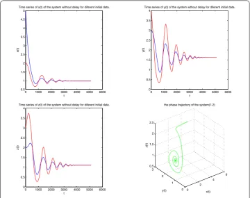
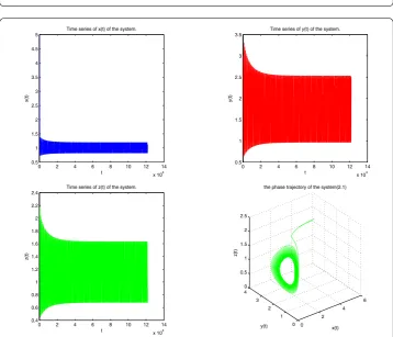
() Whenτ> , according to Theorem ., system (.) undergoes a Hopf bifurcation at the equilibriumE∗whenτ=τ. By directly computing we can obtainτ≈., and the positive equilibrium isE∗(., ., .). We chooseτ = . <τ, and thenE∗ is locally asymptotically stable (see Figure ); On the contrary, we chooseτ= . >τ, and thenE∗ is unstable (see Figure ).

By Theorem . we know that, under the set of parameters, whenτ =τ, a Hopf bifur-cation occurs. Furthermore, we can obtain thatμ> ,β< , the bifurcating periodic

(11)

Figure 2 The positive equilibriumE∗of system (1.2) is locally asymptotically stable whenτ= 0.5 <τ0.

(12)

solutions exist, and the corresponding periodic orbits are orbitally asymptotically stable (see Figure ).

5 Conclusion

A predator-prey-mutualist model is studied in this paper. To be more realistic, it is very necessary to introduce the digestion delay. We consider the asymptotic stability of the positive equilibrium whenτ= ; In addition, whenτ > , the stability of the positive equi-librium and the existence of Hopf bifurcation are studied; we also discuss the direction and stability of Hopf bifurcation. Some numerical analysis is ﬁnally given.

Competing interests

The authors declare that they have no competing interests.

Authors’ contributions

Both authors contributed equally to the writing of this paper. The authors read and approved the ﬁnal manuscript.

Acknowledgements

We are grateful to the editor and reviewers for their valuable comments and suggestions that greatly improved the presentation of this paper. This work is supported by Natural Science Foundation of Shanxi province (2013011002-2).

Received: 2 January 2016 Accepted: 22 June 2016

References

1. Bentley, BL: Extrafloral nectarines and protection by pugnacious bodyguards. Annu. Rev. Ecol. Syst.8, 407-427 (2003) 2. Addicott, JF: A multispecies aphid-ant association: density dependence and species-specific effects. Can. J. Zool.57,

558-569 (1979)

3. Way, MJ: Mutualism between ants and honeydew-producing Homoptera. Annu. Rev. Entomol.8, 307-344 (1963) 4. Rai, B, Freedman, HL, Addicott, JF: Analysis of three species model of mutualism in predator-prey and competitive

systems. Math. Biosci.65, 13-50 (1983)

5. Xiang, H, Su, KS, Jiang, HM, Huo, HF: Qualitative analysis of a mutualistic model with saturating terms and eﬀects of toxic substances. J. Lanzhou Jiaotong Univ.29, 142-145 (2010)

6. Wu, MJ: Positive periodic solutions to a mutualism model with saturating term and the eﬀects of toxic substance. J. Jiamusi Univ.31, 272-274 (2013)

7. Yang, LY, Xie, XD, Chen, FD, Xie, YL: Permanence of the periodic predator-prey-mutualist system. Adv. Diﬀer. Equ.

2015, 331 (2015)

8. Huo, HF, Su, KS, Meng, XY: Permanence and periodic solution of a class of non-autonomous mutualistic system with stage-structure. J. Lanzhou Univ. Technol.36, 128-132 (2010)

9. Rai, B, Krawcewicz, W: Hopf bifurcation in symmetric conﬁguration of predator-prey-mutualist systems. Nonlinear Anal.71, 4279-4296 (2009)

10. Gaines, RE, Mawhin, GL: Coincidence Degree, and Nonlinear Diﬀerential Equations. Lecture Notes in Mathematics, vol. 568, pp. 40-45. Springer, Berlin (1997)

11. Hale, JK, Verduyn Lunel, SM: Introduction to Functional Diﬀerential Equations. Springer, New York (1993)

12. Hassard, B, Kazarinoﬀ, D, Wan, Y: Theory and Applications of Hopf Bifurcation. Cambridge University Press, Cambridge (1981)