Evidence for an elevated 410 km discontinuity below the Luzon, Philippines
region and transition zone properties using seismic stations
in Taiwan and earthquake sources to the south
C. Wright and B.-Y. Kuo
Institute of Earth Sciences, Academia Sinica, P.O. Box 1-55, Nankang, Taipei, Taiwan 11529
(Received May 22, 2006; Revised October 24, 2006; Accepted March 12, 2007; Online published June 27, 2007)
Pwaves from earthquakes south of Taiwan, recorded by seismic stations within and around Taiwan, were used to define two average wavespeed models WPSP01 and WPSP02 for the upper mantle and transition zone below the Luzon region. Wavespeeds are characteristic of oceanic upper mantle. The 410-km discontinuity, however, appears to be elevated to about 325 km depth, based on clear identification of the travel-time branch produced by refraction within the transition zone, and estimates of its first and second derivatives with respect to distance. A plausible explanation is low temperatures within the subducted South China Sea plate. The data also imply relatively low wavespeed jumps of 0.6–1.0% and 1.1–1.5% respectively across the elevated 410-km discontinuity and a lower discontinuity at 676 km depth, and high wavespeed gradients in the transition zone. Phase-weighted stacking on a cluster of short-period seismograms with first arrival energy from within the transition zone provides independent support for the validity of the models; later arrivals are detected close to the predicted times and slownesses for energy emerging from the lowermost upper mantle and the top of the lower mantle. An additional arrival on the stacks may be caused by a localized discontinuity near 530 km depth.
Key words:Philippine Sea plate, Luzon, upper mantle, transition zone.
1.
Introduction
The existence of two major discontinuities at depths of about 410 and 660 km that define the top and bottom of the transition zone was established over 40 years ago (Niazi and Anderson, 1965). Since that time, numerous studies of this region have been published, often using refracted P waves (e.g. Simpson et al, 1974; Walck, 1984; Kaiho and Ken-nett, 2000; Kato and Nakanishi, 2000; Simonet al., 2002), sometimes refractedSwaves (e.g. Ibrahim and Nuttli, 1967; Simon et al., 2003) or surface waves (e.g. Anderson and Toks¨oz, 1963), whilst more recent studies include the use of
P-to-SV orSV-to-P conversions of upgoing seismic body waves at the discontinuities, ScS reverberations, and pre-cursors toPPandSSphases (e.g. Vinnik, 1977; Revenaugh and Jordan, 1991; Shearer and Flanagan, 1999; Li et al., 2000). While these discontinuities have been explained in terms of the phase transformations expected in olivine, py-roxenes and garnets (Ringwood, 1991), there are still diffi-culties in reconciling the wavespeed and density models ob-tained from seismology with the properties of the mineral phases established from experimental petrology and min-eral physics (Anderson and Bass, 1984; Bass and Ander-son, 1984; Fujisawa, 1998; Nishihara and Takahashi, 2001; Bass and Schilling, 2003). Moreover, there are still many regions of the earth, especially in oceanic regions, for which knowledge of the structure of the upper mantle and
transi-Copyright cThe Society of Geomagnetism and Earth, Planetary and Space Sci-ences (SGEPSS); The Seismological Society of Japan; The Volcanological Society of Japan; The Geodetic Society of Japan; The Japanese Society for Planetary Sci-ences; TERRAPUB.
tion zone is poor. Estimates of the wavespeed and density changes across the discontinuities are often poorly resolved, and accurate definition of wavespeed gradients within the transition zone has rarely been obtained.
Two possible petrological models for the upper mantle and transition zone are debated. The more widely accepted olivine-rich pyrolite model (Ringwood, 1962, 1991; Fuji-sawa, 1998) explains the overall density change across the transition zone, but does not provide good agreement with either the estimated wavespeed change across the 410 km discontinuity or the wavespeed gradients within the transi-tion zone (Duffy and Anderson, 1989; Duffyet al. 1995; Li
et al., 1998). Several authors have argued that the alterna-tive pyroxene- and garnet-rich piclogite model (Anderson and Bass, 1984; Bass and Anderson, 1984) explains the ob-served seismic properties within and adjacent to the transi-tion zone as well as the pyrolite model (Duffy and Ander-son, 1984; Ita and Stixrude, 1992; Nishihara and Takahashi, 2001). Considerable uncertainty therefore still remains in using models from seismology to constrain mantle proper-ties and composition.
While the two major discontinuities at about 410 km and 660 km depth are widespread over most of the earth, vari-ations in depths and properties due to the localised lower temperatures and more mafic compositions of subduction zones have been identified. In subduction zones, phase transformation boundaries and mineral assemblages may differ due to the presence of water as well as differences in temperature and composition from the surrounding man-tle (Okamoto and Maruyama, 2004). In cold, subducting
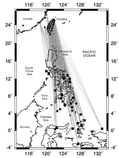
Fig. 1. Map showing stations used in the present study. Diamonds sig-nify broad-band stations of the BATS array, and triangles short-period stations of the CWB network.
slabs in which thermodynamic equilibrium has occurred, the olivine-β phase-spinel phase boundaries may be el-evated (positive Clapeyron slope or exothermic reaction) while the 660 km discontinuity may be depressed (nega-tive Clapeyron slope or endothermic reaction) (Li et al., 2000). Numerical modelling studies that use the proper-ties of the olivine-β phase-spinel phase boundary as part of the process of calculating the stress regime and depths of phase transformations in subducting slabs (Schmelinget al., 1999; Negredoet al., 2004), predict that the depth of the 410 km discontinuity may be elevated by 70 km or more. Seismological observations have been used to estimate a 60 km elevation of the olivine-βphase-spinel boundary in the Izu-Bonnin subduction zone (Collier and Hellfrich, 1997), a smaller elevation of 20 km has been reported in a conti-nental region (Chen et al., 1997), and other examples are given in Wright (2007).
The 660 km discontinuity is known to be anomalously deep around some subduction zones (Liet al., 2000). ForP
waves, the discontinuity is also poorly defined below parts of southern Africa (Zhaoet al., 1999; Simonet al., 2002) and apparently absent below the Himalayan region (Ram and Mereu, 1977), suggesting that the properties of the lower part of the transition zone may vary regionally away from those regions where subduction is currently taking place.
The aim of this work is to derive average P wave mod-els of the upper mantle and transition zone beneath the western margin of the Philippine Sea plate around Luzon. Emphasis is on the seismological evidence to explain the travel-time anomalies that exist in the region, which was previously studied by Nowacket al. (1999). The geody-namic consequences of the results are explored by Wright (2007). Earthquakes recorded by the broad-band BATS ar-ray (Broad-band Arar-ray in Taiwan for Seismology) and the
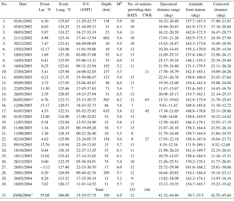
Fig. 2. Map showing distribution of events used to determine mantle struc-ture, with great circle paths (dotted grey lines) to the stations providing seismograms for each event. Squares and stars denote events at depths of 150 km or less and depths greater than 150 km, respectively.
short-period CWB (Central Weather Bureau) seismic net-work (Fig. 1) provided refracted arrivals to define man-tle structure between depths of 100 and 800 km. An im-portant focus of the work, due to limitations of the avail-able data, is on the information on structure provided by travel-time measurements. Such data provide constraints on the depths of major discontinuities, the wavespeed changes across discontinuities and wavespeed gradients within the transition zone. The models have been tested by stacking seismograms to identify later arrivals associated with the triplications produced by the inferred discontinuities. Fur-ther refinements, to be explored in a later paper, involve the comparison of the signal waveforms with synthetic seismograms, and the development of complex, laterally-varying and frequency-dependent earth models for the re-gion around Taiwan, which rely on the initial development of a robust one-dimensional model.
2.
Selection of Data
The distribution of seismicity around Taiwan suggests the construction of three roughly linear profiles to examine the structure of the upper mantle and transition zone in the re-gion: to the north-east along the Ryukyu arc (azimuths 30◦– 60◦ from central Taiwan), to the south along the western margin of the Philippine Sea plate (azimuths 150◦–190◦) and possibly a more diffuse profile to the west across east-ern Asia (azimuths 260◦–305◦). The present work is con-cerned with the second of these profiles to the south of Tai-wan.
Table 1. Earthquakes used for determining mantle structure.
No. Date Event Event O.T. Depth M# No. of stations Epicentral Azimuth Corrected
Lat.◦N Long.◦E (GMT) (km) providing data distance range from station distance
BATS CWB (deg) (deg) (deg)
1. 01/01/2002 6.30 125.65 11-29-22.73 138 5.9 10 16.23–20.48 157.7–167.5 17.80–21.91
2. 05/03/2002 6.03 124.25 21-16-09.13 31 6.3 10 16.96–20.43 161.9–172.5 17.18–20.64
3. 08/03/2002 5.87 124.27 18-27-53.19 23 5.6 11 16.32–20.59 162.0–172.5 16.47–20.73
4. 21/12/2002 4.98 123.16 17-41-13.54 602 5.4 10 17.01–21.28 165.9–175.3 24.10–27.94
5. 30/12/2002 7.47 123.41 04-49-08.69 10 5.9 10 15.43–18.87 163.3–173.8 15.49–18.94
6. 15/02/2003 12.17 124.08 11-01-59.86 10 5.8 13 10.20–14.45 155.2–170.0 10.29–14.54
7. 10/03/2003 1.69 127.30 02-09-37.08 93 6.2 13 21.09–25.33 157.8–166.3 21.98–26.12
8. 14/03/2003 0.41 132.95 07-06-13.31 33 6.0 13 25.17–29.24 148.1–155.3 25.34–29.40
9. 16/04/2003 0.25 122.01 09-31-23.94 192 5.2 11 21.59–24.80 171.1–179.5 23.11–26.28
10. 27/04/2003 5.41 125.98 16-08-42.03 137 5.3 11 17.58–18.79 162.5–165.1 19.09–20.26
11. 05/05/2003 0.22 127.35 15-50-08.47 123 5.9 13 22.51–26.76 158.8–166.9 23.42–27.64
12. 05/05/2003 3.72 127.95 23-04-45.67 56 6.0 13 19.39–23.60 154.4–163.4 19.88–24.04
13. 22/05/2003 11.30 125.46 17-45-37.63 71 5.4 7 11.47–15.67 151.6–165.1 14.45–16.76
14. 26/05/2003 2.35 128.85 19-23-27.94 31 6.5 12 20.98–25.17 153.7–162.1 21.14–25.33
15. 26/05/2003* 6.76 123.71 23-13-29.72 565 6.2 12 63 15.33–19.62 162.9–175.0 21.79–25.83
16. 12/06/2003 13.17 120.51 18-43-32.73 46 5.6 7 9.61–11.42 169.4–185.6 11.10–12.72
17. 01/07/2003 4.53 122.51 05-52-25.92 635 5.8 12 45 17.38–21.65 168.0–178.8 25.11–28.86
18. 01/07/2003 12.80 124.90 17-00-22.82 33 5.6 13 9.88–14.08 150.8–165.9 10.23–14.42
19. 11/07/2003 9.34 122.04 13-53-24.90 33 5.6 13 12.58–16.85 166.3–179.1 12.92–17.19
20. 11/08/2003 1.14 128.15 00-19-09.28 10 5.7 13 21.87–26.10 156.3–164.6 21.93–26.14
21. 11/08/2003 1.26 128.19 00-22-26.40 10 5.5 8 21.79–24.48 159.7–164.4 21.84–24.53
22. 02/10/2003 4.62 125.98 23-24-05.75 154 5.0 8 27 17.93–22.18 158.4–167.6 19.64–23.72
23. 09/10/2003 13.76 119.94 22-19-13.85 33 5.7 13 8.18–12.34 171.9–189.1 8.52–12.68
24. 18/10/2003 0.44 126.10 22-27-13.25 33 6.1 11 21.98–26.24 161.4–169.7 22.15–26.41
25. 18/11/2003 12.02 125.42 17-14-22.62 35 6.1 13 10.79–14.97 150.4–164.5 11.16–15.31
26. 28/12/2003 0.60 122.35 05-36-54.81 74 5.4 10 21.26–25.51 170.2–178.1 21.77–26.01
27. 28/01/2004 −3.12 127.40 22-15-30.70 17 6.0 12 25.72–29.98 161.0–168.2 25.81–30.06
28. 29/01/2004 6.29 126.94 09-48-42.76 209 5.7 12 16.64–20.85 154.1–164.4 19.14–23.11
29. 26/02/2004 8.29 123.52 17-25-56.19 12 5.2 9 13.82–18.09 162.2–174.1 13.93–18.18
30. 16/05/2004 7.63 126.17 11-01-14.52 11 5.7 11 15.13–19.35 154.7–165.7 15.23–19.42
Total 323 146
31. 10/06/2004+ 55.68 160.00 15-19-57.75 189 6.9 12 41.32–44.46 30.7–33.5 42.55–45.64
#Event magnitude.
∗ScP times also picked for estimating station corrections. +Teleseismic event—times used for estimating station corrections.
on islands close to mainland China (Fig. 1). The array is run by the Data Management Centre, Institute of Earth Sci-ences (IES), Academia Sinica, and the data are telemetered by radio to the IES building in eastern Taipei. Records from 30 earthquakes at distances between 8◦ and 30◦, azimuths between 150◦ and 190◦, and magnitudes greater than 5.0 recorded at stations of the BATS array were selected from the data base of the Institute of Earth Sciences, Academia Sinica, for the years 2002–2004 (Fig. 2 and Table 1). Data were recorded at 20 Hz sampling rate and preliminary pro-cessing undertaken using SAC (Seismic Analysis Code) software for 13 of the stations; one station, LYUB, was too noisy to give useful data.
While the BATS array provides high-quality broad-band records, the denser CWB network, equipped with Teledyne-Geotech S-13 short-period seismometers, whose function is to provide information on local seismicity, may provide ad-ditional constraints on deep structure, and was previously used for this purpose by Nowack et al. (1999). Records were extracted from the CWB database by staff of the In-stitute of Earth Sciences, Academia Sinica, and archived
at a 100 Hz sampling rate for later processing using SAC. 4 events were selected to determine how effective the data would be in supplementing the BATS data for defining the structure of the upper mantle and transition zone (Table 1), and provided data from 63 of the 75 stations of the net-work. Records from earthquakes outside the Taiwan region are discarded from the CWB database about 12 months after their occurrence, unless researchers arrange to save them. The amount of data from CWB stations currently available for this kind of study is therefore limited.
3.
Methods of Data Analysis
3.1 Character of seismograms
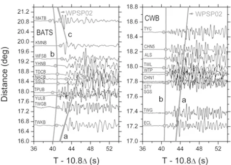
Fig. 3. Seismograms for event 28 of Table 1 at 11 BATS stations (left) and 10 CWB stations used to construct phase-weighted stacks plotted as epicentral distance against reduced travel time. Station corrections (Fig. 4) were applied prior to plotting. Data from the BATS stations were used in deriving models WPSP01P and WPSP02P, whilst data from the CWB stations were used only for generating phase-weighted stacks. The travel-time curve computed from model WPSP02 has been superimposed after applying a ‘baseline’ shift of 0.92 s (the ‘event bias correction’ for the event). Travel-time branches ‘a’, ‘b’ and ‘c’ are labelled, and explained in the caption to Fig. 5. Because the event was at a depth of 209 km, the cross-over point between branches ‘a’ and ‘b’ at 17.7◦distance for an event on the surface has been shifted back to 14.2◦.
Fig. 3. All data were filtered with a bandpass of 0.4–5.0 Hz, which makes the waveforms of adjacent BATS and CWB stations very similar. The seismograms from CWB stations for this event were not used in deriving the wavespeed mod-els, and were chosen as good examples for presentation be-cause they have clear arrivals from a fairly deep event (209 km depth), have energy from the transition zone as the first arrival for all stations, and, with signal processing, yield in-formation on later arrival branches. Circles mark the picked arrival times at the BATS and CWB stations, and all times of onsets and seismograms were corrected using the station corrections of Fig. 4.
The travel-time curve calculated from model WPSP02 (Figs. 5 and 6) is superimposed on the record sections with a time shift of 0.92 s (the ‘event bias correction’ for the event defined in Section 4). Observed travel times can be divided into three main arrival branches (Fig. 5) denoted ‘a’ (refracted paths through the upper mantle), ‘b’ (refracted paths through the transition zone), and ‘c’ (refracted paths through the lower mantle), with ‘b’ as the first arrival for all seismograms in Fig. 3. At TWKB and CWB station ECL, there is a strong later arrival that matches branch ‘a’. Stations KMNB and MATB have especially clear arrivals due to their location on stable continental crust close to the Chinese mainland. In particular, the P wavetrain at MATB shows two clear arrivals that can be attributed to branches ‘b’ and ‘c’. However, for stations on or close to the island of Taiwan, there are large variations in waveform, even at closely-separated stations, due to the complicated underlying lithospheric structure. This makes it difficult to reliably identify the later arrival branches without the careful processing described in Section 6.
Fig. 4. Station corrections for CWB (top) and BATS stations (bottom), with stations arranged from west to east.
3.2 Focal depth and station corrections
Arrival times of the earliest P wave arrivals measured on records bandpass-filtered between 0.4 and 5.0 Hz were the primary input data. All distances and times were cor-rected by ray tracing to make each event appear to be lo-cated on the surface. The slownesses used for making the corrections were derived from the IASPEI 1991 Seismolog-ical Tables (Kennett, 1991), and the IASP91P wavespeed model from the tables was adopted for the ray tracing. An important step in the interpretation was to ensure that each arrival time was attributed to the correct travel-time branch ‘a’, ‘b’ or ‘c’ prior to making the correction. Errors in the corrected distances and bias in slowness due to the differ-ences between the local structure and the reference model are small (see Section 9). However, errors in the total travel times, which can be significant if an inappropriate reference model is chosen, are largely eliminated later by absorption into the ‘event bias corrections’.
com-Fig. 5. (Top) Reduced travel-time curve for the IASP91 model of Ken-nett (1991), with measured first arrival times adjusted to their sur-face-to-surface equivalents; (bottom) sursur-face-to-surface times with both station corrections and ‘event bias corrections’ applied, and curve fits for branches ‘a’ (refracted arrival from the upper mantle), ‘b’ (re-fracted arrival from within the transition zone) and ‘c’ (re(re-fracted arrival from within the lower mantle). Travel times computed from models WPSP01P and WPSP02P are superimposed on the estimated travel-time branches to show how well the model-generated times fit the data.
plex three-dimensional model assembled from earlier stud-ies, whose reliability would be difficult to assess. The procedure involved first calculating the travel-time residu-als relative to the arrival times predicted from the IASP91 model (Kennett, 1991) for times attributed to branch ‘c’ (i.e. arrivals from signals that had penetrated to lower mantle depths). Figure 5 shows the travel-time curves calculated by ray tracing for a surface event recorded at locations on the surface using the IASP91 model (top) and the models de-rived in this study (bottom). Significant distance-dependent differences in earth structure from those of the reference model (IASP91) are assumed to be absent from time mea-surements of branch ‘c’ that were first arrivals. With this assumption, 5 events (events 4,8,15,17 and 27 of Table 1) were available to provide estimates of station corrections. The data were supplemented by times from one teleseism (last event in Table 1) and theScPtimes from event 15.
A least-squares inversion was then performed to estimate a station correction for each of the 13 stations of BATS and a ‘bias’ term for each earthquake, consisting of the com-bined errors in origin time and correction for focal depth, and the effect of real deviations in earth structure from the reference model. Two separate bias terms were calculated
Fig. 6. (Left) Pwavespeed models WPSP01P and WPSP02P; (Right)
Pwavespeed model WPSP01P with 95% confidence limits on wavespeed estimates.
for event 15, because the P andScParrivals travelled dif-ferent paths, and therefore the effects of deviations from the reference model were unrelated. This resulted in 83 vations for estimating 20 parameters. Because the obser-vations used in the least-squares inversion consisted of dif-ferences between the parameters that were being estimated, one parameter (the station correction for KMNB near the Chinese mainland) was set to zero. KMNB was chosen be-cause it is a reliable station away from the structural com-plexities of Taiwan, and is also the reference station used by Chenet al.(2004). The station corrections and estimated standard errors are plotted in the lower half of Fig. 4, not-ing that the estimated standard deviation on a snot-ingle differ-ence between a station correction and an event ‘bias’, σ, was 0.64 s. As a check, the inversion was also undertaken for the remaining times belonging to branches ‘a’ and ‘b’ (264 observations for estimating 37 parameters), although complex deviations from the reference model were clearly present, making good agreement with the earlier results un-likely. Nevertheless, satisfactory agreement with the results of Fig. 4 was obtained for 9 of the 13 stations, but the stan-dard deviation,σ, increased to 1.14 s.
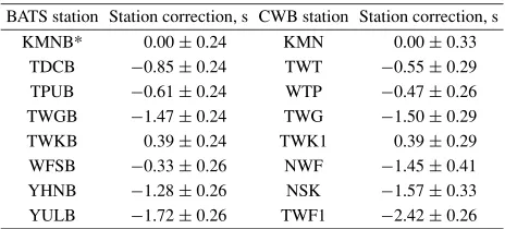
A similar analysis was also undertaken for the three events recorded by CWB stations that gave times for branch ‘c’, supplemented by theScPtimes for event 17 (209 ob-servations for estimating 67 parameters, 63 of them station corrections). Despite the large number of stations and rela-tively small number of observations, the station corrections at CWB stations at locations within 10 km of a BATS sta-tion were in satisfactory agreement with their BATS coun-terparts (Table 2). Furthermore, the general regional trend of CWB station corrections shown in the upper part of Fig. 4 was in satisfactory agreement with the results from BATS, while the standard deviation,σ, was 0.57 s.
4.
Corrections for Errors in Origin Times
(Event-bias Corrections)
com-Fig. 7. Method of determining ‘event bias corrections’.
bined errors in origin times and corrections for focal depth that were used for separating station corrections. The input times have already been corrected for station effects, and the new set of corrections are estimated independently of any reference travel-time curve. The principle of the method is illustrated in Fig. 7.
The first step was to fit a separate line or a quadratic poly-nomial through the arrival times from each of the 30 earth-quakes used, adjusted to correspond to surface-to-surface paths. A quadratic form was used only if there was an im-provement in fit (10 % reduction in standard deviation on time residuals) over the linear form. To check the value of using station corrections, the curve fitting was undertaken using times from both BATS and CWB stations first with, and then without application of station corrections. The ap-plication of station corrections resulted in improved fits for 22 of the 30 events, with the worse fits concentrated at short distances where the scatter of the times is greatest. There is a gradual decrease in the standard deviation on the time residuals on the curve fits to the times with station correc-tions for each event from about 1.5 s at the shortest dis-tances to about 0.6 s on average for the times on branch ‘c’ at the largest distances, indicating less effects of inhomo-geneity as the seismic energy travels deeper paths. The re-sults therefore showed the necessity of undertaking all com-putations on times with the station corrections applied.
After the curve fitting, the following procedure was used for deriving ‘event bias corrections’. Consider the curve fit to the times for a particular earthquake j (Fig. 7). Time residuals from all other earthquakes relative to this curve, for which seismograms lie within the distance range of the stations recording this earthquake, were used to calculate an average residual for each event, provided that at least two stations were within this distance range. This is represented in Fig. 7 by the times tj−1,j, tj+1,j tj+2,j, which define
the average time residuals from earthquakes j −1, j +1 and j +2 relative to a reference event j. This process was repeated using all earthquakes as the reference event, and the average residuals provided input data to estimate relative origin time errors using a weighted least-squares inversion procedure; the weight for each average residual was the number of degrees of freedom (n−1, wheren is the number of residuals used to compute the average). The method was previously used by Simon et al. (2002) and Wrightet al.(2002), and the mathematical details provided
Table 2. Comparison of station corrections at BATS and CWB stations separated by less than 10 km.
BATS station Station correction, s CWB station Station correction, s
KMNB* 0.00±0.24 KMN 0.00±0.33
TDCB −0.85±0.24 TWT −0.55±0.29
TPUB −0.61±0.24 WTP −0.47±0.26
TWGB −1.47±0.24 TWG −1.50±0.29
TWKB 0.39±0.24 TWK1 0.39±0.29
WFSB −0.33±0.26 NWF −1.45±0.41
YHNB −1.28±0.26 NSK −1.57±0.33
YULB −1.72±0.26 TWF1 −2.42±0.26
*For stations KMNB and KMN, the station corrections were set to zero, as described in the section on the least-squares inversion.
by Wright (2006).
The ‘event bias corrections’ are reliably-determined pa-rameters having standard errors in the range 0.07–0.21 s. Because the inversion is undertaken on differences, one earthquake has to be taken as a reference, and its correc-tion set to zero. Event 17 of Table 1 was chosen as the reference, since it provided clear arrivals at both the BATS array and CWB network, with all times belonging to branch ‘c’ of Fig. 5. After applying station corrections, taking both KMNB (BATS) and KMN (CWB) (7.6 km from KMN) to have values of zero (Table 2), the mean travel-time resid-ual of this event relative to the IASPEI travel times was 0.67 s. Since the travel-time residuals on the times for all events relative to IASPEI are, on average, slightly earlier for branch ‘c’ at larger distances (Fig. 5), and become progres-sively later as the distance decreases along branches ‘b’ and ‘a’, no further refinement of the choice of reference time can be made. Later observed times relative to the IASPEI times at short distances are expected for any region of oceanic mantle, since the reference times were generated by a model that is a weighted average of oceanic and faster continental wavespeeds.
After applying the ‘event bias corrections’, the new set of travel times used to derive models had the following proper-ties: (i) corrected for errors in origin times, in time correc-tions for focal depth, and for station effects, but uncertain by a constant which was defined to give times at 28◦ dis-tance, slightly later than the IASPEI times; (ii) defined in-dependently of any reference travel-time curve, apart from the tie to IASPEI times at 28◦. The accuracy of the long-wavelength variations in these travel times depends on the density of travel-time measurements, the amount of overlap in distance range of the events, and the amount of lateral heterogeneity over the region studied. The application of ‘event bias corrections’ also suppresses any time anomalies produced at shallow depths in the source region. Cumu-lative errors in ‘event bias corrections’ between distances of 8.5◦and 30.0◦ are estimated to be less than one second. The physical basis and significance of the ‘event bias cor-rections’ are discussed further in Appendix B.
5.
Construction of a Preliminary Earth Model
Table 3. Definition of travel-time branches ‘a’, ‘b’ and ‘c’.
Branch Polynomial coefficients No. of Distance Standard
data points range (deg) deviation (s)
a 2.90399 s (t0) 15.2855 (t1) 123 8.52–18.94 1.33
−7.79730×10⁻²s−1(t2)
b −2.51117 s (t0) 16.6843 (t1) 211 17.10–24.92 0.86
−9.94385×10⁻²s−1(t2)
c 58.6205 s (t0) 12.8536 (t1) 246 21.79–30.06 0.73
−1.04426×10⁻²s−1(t2)
7.76591×10⁻⁴s−2(t3)
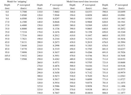
Table 4. PreliminaryPmodel WPSP02P (Western Margin, Philippine Sea Plate 02—Pwaves) constructed to fit branches ‘a’, ‘b’ and ‘c’.
Model for ‘stripping’ Model from travel-time inversion
Depth Pwavespeed Depth Pwavespeed Depth Pwavespeed Depth Pwavespeed
(km) (km/s) (km) (km/s) (km) (km/s) (km) (km/s)
0.0 5.7500 110.0 7.9602 340.0 8.8353 590.0 10.0499
9.0 5.8500 120.0 7.9948 350.0 8.8858 600.0 10.0981
9.0 6.0500 130.0 8.0297 360.0 8.9363 610.0 10.1463
17.0 6.1500 140.0 8.0646 370.0 8.9868 620.0 10.1941
17.0 6.4000 150.0 8.0993 380.0 9.0369 630.0 10.2407
35.0 6.8000 160.0 8.1336 390.0 9.0865 640.0 10.2852
35.0 7.7218 170.0 8.1676 400.0 9.1358 650.0 10.3240
45.0 7.7516 180.0 8.2012 410.0 9.1847 660.0 10.3555
55.0 7.7821 190.0 8.2344 420.0 9.2334 670.0 10.3836
65.0 7.8131 200.0 8.2673 430.0 9.2819 676.0 10.3994
75.0 7.8448 210.0 8.2998 440.0 9.3303 676.0 10.5571
85.0 7.8770 220.0 8.3319 450.0 9.3785 681.0 10.6237
95.0 7.9098 230.0 8.3637 460.0 9.4266 691.0 10.7026
105.0 7.9432 240.0 8.3951 470.0 9.4746 701.0 10.7648
109.6 7.9588 250.0 8.4262 480.0 9.5226 711.0 10.8193
260.0 8.4571 490.0 9.5705 721.0 10.8688
270.0 8.4876 500.0 9.6184 731.0 10.9146
280.0 8.5178 510.0 9.6663 741.0 10.9575
290.0 8.5458 520.0 9.7142 751.0 10.9979
300.0 8.5673 530.0 9.7620 761.0 11.0363
310.0 8.5817 540.0 9.8099 771.0 11.0727
320.0 8.5934 550.0 9.8578 781.0 11.1075
325.0 8.5986 560.0 9.9058 791.0 11.1406
325.0 8.7594 570.0 9.9538 801.0 11.1723
330.0 8.7847 580.0 10.0018 806.0 11.1877
events. The cross-over distances between the branches were resolvable by visual inspection of the corrected times, but were confirmed by locating the point of inflection of the slowness relation estimated from these times (see Section 9 and figure 3 of Wrightet al., 1985). Because the location of the nearer cross-over distance is especially important for the definition of the 410-km discontinuity, further discus-sion is provided in Appendix A. Travel-time curves were fitted to the three branches with a small amount of over-lap. The identification of these branches implies the exis-tence of both the 410- and 660-kilometre discontinuities. The branches ‘a’, ‘b’ and ‘c’ were found to be satisfacto-rily fitted with quadratic, quadratic and cubic polynomials respectively (Fig. 5 and Table 3). Branch ‘c’ was defined for corrected distances from 21.8◦–30.1◦, so that the obser-vations extend 2.4◦back from the cross-over point for first arrivals through the times for event 15 at a depth of 565 km (Table 1). For this event, branch ‘b’ was not observed,
since the slope of the first arrivals shows that they belong to branch ‘c’ (Fig. 5). The final models WPSP01 and WPSP02 predict that branch ‘b’ should be the earliest arrival over part of the distance range of this event. However, failure to ob-serve branch ‘b’ could have several explanations, including incorrect focal depth and radiation pattern effects, and does not necessarily imply that there is a problem with the final models.
mantle (Table 4, left two columns). The model provides travel times and slownesses that fit smoothly on to branch ‘a’ at a distance of 10.0◦where the data coverage becomes reasonably dense. This corresponds to a depth of 109.8 km and a wavespeed of 7.959 km/s. The model was used to ‘strip’ the earth to a depth of 110 km, and the Herglotz-Wiechert integral (Shearer, 1999, pp. 66–67) was used to determine a wavespeed model to a depth of 500 km, by ex-trapolating the slowness curve of branch ‘a’ to a distance of 25◦. The resulting model was then used to ‘strip’ the earth to several depths between 320 km and 400 km, and the Herglotz-Wiechert integral undertaken along branch ‘b’ extrapolated to distances of 26◦. For each depth, the start-ing distance for the new integration was calculated durstart-ing the stripping process. When the best fit for the depth of the assumed first-order discontinuity had been obtained (325 km), the earth was stripped to that depth and the Herglotz-Wiechert integral evaluated along branch ‘b’ extrapolated to a distance of 30◦to give wavespeed models to depths of about 800 km. The new model was then used to ‘strip’ the earth to several depths between 640 and 680 km. Herglotz-Wiechert integration was then undertaken along branch ‘c’ and ray tracing used to select the depth of the discontinuity that gave the best fit to the observed times (676 km). The preliminary model WPSP01P resulting from these compu-tations is shown in Fig. 6.
Model WPSP01P shows small wavespeed jumps across the discontinuities at depths of 325 and 676 km compared with many other published models of the transition zone (0.6% and 1.1% respectively, compared with 3.6% and 5.8% respectively in the IASP91 model of Kennett, 1991, for example). This situation arises because of the mea-sured gradients of branches ‘a’, ‘b’ and ‘c’ in the distance ranges in which they are first arrivals; when these gradi-ents are extrapolated into the region in which they are later arrivals, they imply small wavespeed jumps across both dis-continuities. The wavespeed gradients within the transition zone (Fig. 6), which were defined by the first arrivals (cor-responding depths 361–608 km) are high compared with many other models. The wavespeed gradients may be lower both above and below the two discontinuities than the de-rived slowness curves suggest, but the reduced gradients of the branches of the slowness curves would be difficult to estimate from later arrivals. If this were true, the changes in wavespeed at each discontinuity permitted by the travel times would be larger. To test this idea, the slowness curves for branches ‘a’ and ‘b’ were changed in the regions in which they were second arrivals to have lower gradients. Slowness curves of branches ‘a’ and ‘b’ are defined by lin-ear forms. At the crossover distance of 17.7◦, the slowness gradients were reduced by changing to quadratic forms on both the high- and low-distance sides of the cross-over for branches ‘a’ and ‘b’ to bend the gradients to lower values over a distance range of 1◦, and then return to a linear form. Continuity of both the slowness and its first derivative were imposed. No attempt, however, was made to change the slowness gradient of branch ‘c’ at distances less than the cross-over at 24.2◦, since the gradient was defined by ob-servations in this distance range from event 15 of Table 1. However, the slowness gradient of branch ‘b’ was reduced
at distances greater than 24.2◦, where it was a later arrival. The modified slowness curves suggest that the increases in wavespeed across the upper and lower discontinuities can be increased to 1.0% and 1.5% respectively, which are still lower than in many published models, due to the high esti-mated wavespeed gradients in the transition zone.
6.
Identifying Later Branches Associated with
Triplications
The broad-band stations of the BATS array are too far apart to allow the effective use of stacking techniques to enhance later arrivals. The alternative is to use the more densely-spaced stations of the short-period CWB network. Finding data of sufficient quality to allow a search for branches ‘a’ and ‘c’ as later arrivals, with usable seismo-grams giving branch ‘b’ as the first arrival, was difficult. The most suitable event for this purpose is event 28 of Ta-ble 1, in which branch ‘b’ was the first arrival at all sta-tions. The chosen event often showed a weakParrival fol-lowed by a stronger P arrival about 2 seconds later. This phenomenon is well illustrated by the BATS seismograms in the left section of Fig. 3, where very small, but distinct early arrivals can be identified at stations YHNB and TDCB (too small to be seen with the scaling of the plot), but not at KMNB or NACB, where the earliest detectable arrival is strong. The earliest detectable energy arriving at NACB is also very late, forming an outlier in the data. The time picks generally lie close to the branch ‘b’, although the scat-ter is somewhat larger than for most other events used in deriving the models. Second arrivals that may be associ-ated with branches ‘a’ and ‘c’ are visible at stations TWKB and MATB, respectively, with an additional strong arrival at WFSB lying close to the linear extension of branch ‘a’. Later phases at the other broad-band stations are not clearly identifiable.
Because they are difficult to observe on single seismo-grams, the later arrival branches associated with triplica-tions caused by discontinuities at transition zone depths have been previously identified by stacking seismograms at dense arrays of seismometers (Simpsonet al., 1974; Ram and Mereu, 1977) or non-linear stacking at a more sparsely distributed network of stations (Simonet al., 2002). Fol-lowing Simon et al. (2002), the phase-weighted stack (Schimmel and Paulsen, 1997) was used to demonstrate the presence of later arrival branches. Effective use of the method, however, requires careful selection and preparation of the data as explained below.
Fig. 8. Set of phase-weighted stacks at slownesses between−2.0 and 1.4 s/deg relative to the slowness of the first arrival branch ‘b’, produced from 11 CWB stations aligned with the P onset for station STY to provide a reference distance of 17.80◦. The small circles define the onset times of signals attributed to branches ‘a’, ‘b’ and ‘c’, and an additional signal ‘?’ 2.1 seconds after thePonset.
to a distance range of less than 1.3◦(17.21◦–18.46◦). These seismograms all showed a small P arrival followed by a stronger signal about 2 seconds later. 10 of them are plot-ted on the right side of Fig. 3 after application of station corrections; the seismogram from CHN4 (distance 18.03◦) was not plotted because no station correction was available. Later arrivals close to the times expected from branch ‘a’ are clear only at ECL and TYC.
Before applying phase-weighted stacking, the seismo-grams were shifted in time to have the same arrival time as the reference station STY (distance 17.80◦). The first four seconds following eachParrival were then cross-correlated with the first four seconds of two of the clearer seismograms (STY and ALS) to define small adjustments to the times of the seismograms that should result in better alignment of later arrivals. The amplitudes of the seismograms were also adjusted to have the same maximum peak-to-trough values over the same four-second period. Phase-weighted stack-ing was then undertaken usstack-ing a phase weightstack-ing index of 3, and a smoothing window of 41 samples (0.4 s), at slow-ness intervals of 0.2 s/deg relative to the aligned traces over the range −2.0 to 1.4 s/deg. The slowness of branch ‘b’ at a distance of 17.80◦ is 11.03 s/deg for model WPSP02, while the slowness estimated from a quadratic polynomial fit to arrival times was 10.74±0.10 s/deg. The difference between the predicted and measured slownesses is largely due to the uneven distribution and small number of stations (Fig. 3).
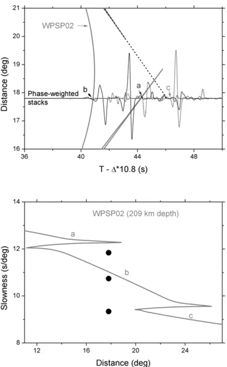
Fig. 9. (Top) ThePtravel-time curve computed from model WPSP02 for an event at a depth of 209 km, after applying a ‘baseline’ shift of 0.92 s to be consistent with Fig. 3, with three phase-weighted stacks plotted on top of each other at the reference distance of 17.80◦. Black, dotted and grey lines correspond to the relative slownesses in Fig. 8 of 0.0, 1.0 and−1.4 s/deg, respectively. The dashed line is the linear extension of branch ‘c’ to a distance of 17.80◦. (Bottom) Slowness curve computed by ray tracing through model WPSP02 for an event at 209 km depth. The dots are the slownesses of the maximum amplitudes of the three signals labelled ‘b’, ‘a’ and ‘c’ in the upper part of the figure.
Figure 8 shows the phase-weighted stacks plotted as a function of travel time. At zero relative slowness, the earli-estParrival energy of branch ‘b’ arrives at a time of 233.5 s, followed by a stronger arrival about 2 s later, with a max-imum amplitude at a slowness 0.2 s/deg lower. There is a signal arriving 3.4 s after the Ponset at a relative slowness of 1.0–1.2 s/deg, which is attributed to branch ‘a’. Then, 5.5 s after P, a strong signal arrives at a relative slowness of−1.4 s/deg, which can be associated with branch ‘c’. The next step is to determine how well the slownesses and times of these arrivals agree with the predictions of one of the de-rived models, WPSP02.
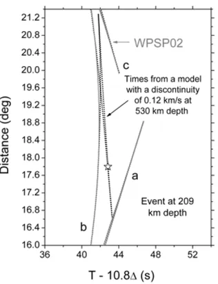
Fig. 10. Reduced travel-time curves from model WPSP02 (grey lines) and a model like WPSP02, but with an additional discontinuity of 0.12 km/s at a depth of 530 km (dotted lines). Travel-time branches are as in the caption to Fig. 5. The star marks the arrival at a distance of 17.8◦ attributed to the additional phase shown in Figs. 8 and 9.
fit branch ‘b’. The trace for a relative slowness of 1.0 s/deg shows an arrival close to the expected time for branch ‘a’. Over the distance range of the stack, the signal should con-sist of interfering refracted and reflected branches whose separations will differ from one input trace to another. The stacked output may therefore be influenced by phase shifts between input signals due to both this interference effect and differences in the curvature of branches ‘a’ and ‘b’. Obvious similarity in the stacked outputs from branches ‘a’ and ‘b’ cannot therefore be expected. Although, on ray the-ory, branch ‘c’ terminates at 19.8◦, wave theory predicts ar-rivals at shorter distances. A strong arrival is observed close to the linear extension of branch ‘c’ to 17.80◦(dotted line), consistent with this idea.
The lower part of Fig. 9 shows the slowness–distance relation for an event at a depth of 209 km depth computed for model WPSP02. The slowness estimates for the arrivals marked ‘a’, ‘b’ and ‘c’ in the top half of Fig. 9 are plotted at a distance of 17.80◦, and show reasonable agreement with the slownesses predicted at that distance by the model. Phase-weighted stacking has therefore identified two later arrivals that agree satisfactorily in both arrival time and slowness with the predictions from model WPSP02.
A possible explanation for the signal marked by a ques-tion mark in Fig. 8 is shown in Fig. 10. The travel-time curve calculated from model WPSP02 is plotted as the con-tinuous grey line, as in Fig. 3. The travel times shown as dotted lines were calculated from a perturbed version of WPSP02. This perturbed model has a discontinuity of 0.12 km/s at a depth of 530 km, in which the wavespeeds were gradually decreased below a depth of 450 km to a value 0.07 km/s less than WPSP02 at 530 km depth. The increased wavespeeds at the discontinuity were tapered to fit on to WPSP02 at 610 km depth. The new model introduces an additional triplication with an arrival 1.1 s later and a slow-ness 0.6 s/deg lower than branch ‘b’ at a distance of 17.8◦,
which is marked by a star. In Fig. 8, the earliest energy of the large arrival marked by a question mark is about 1.6 s after branch ‘b’ (the small pulse before the circle at the onset of the large wavelet), and has a slowness 0.2 s/deg less than that of branch ‘b’. Allowing for the uncertain-ties in the slownesses estimated by phase-weighted stack-ing, the agreement between the theoretical and estimated slownesses is fair, while the observed arrival is late by at least 0.5 s. The time separation between branch ‘b’ and the strong arrival can be increased by making the discontinuity larger or increasing its depth. However, in both cases the difference in slowness would become larger, while the ex-istence of an additional discontinuity within the transition zone that is as prominent as either the 410- or 660-km dis-continuity is not easy to explain.
A relatively small 520-km discontinuity has been re-ported in some regions, mostly from long-period observa-tions (Shearer, 1990; Revenaugh and Jordan, 1991; Flana-gan and Shearer, 1998). It has usually been attributed to the transformation of the β form of olivine to the spinel (γ ) structure (Sinogeikinet al., 2003). However, litte or no evidence for the presence of this discontinuity has come from short-periodP waves (Cumminset al., 1992; Vidale and Benz, 1992). The absence of frequent identifications of the 520-km discontinuity suggests a transition zone with a relatively low olivine content if theβ−γ transition is the cause. However, in instances when subducting slabs flatten above the 660-km discontinuity, a discontinuity near 520 km depth may be caused by majorite garnet above theγ form of olivine (Sinogeikinet al., 2003), giving rise to large
P and S wavespeed increases of up to 6 and 9% respec-tively. Furthermore, the wavespeed gradients in the overly-ing region around the contact between former basaltic crust and average mantle would be low or possibly negative. This phenomenon would also explain the low amplitude of the ‘b’ branch in Fig. 8. The additional phase may therefore be caused by another discontinuity near 530 km depth, local-ized in the vicinity of a sub-horizontal slab, but more data, allowance for the effects of lateral heterogeneity, waveform modelling, and further work on resolving the complicated plate geometry of the region (Wright, 2007), will be re-quired to fully explain its late arrival time and large am-plitude.
7.
Model Uncertainties
The uncertainties in one-dimensional earth models de-rived by inversion of body waves have often been deter-mined (Wigginset al, 1973; Walck, 1984), but by meth-ods that are non-probabilistic in the sense that increasing the number of observations does not reduce the uncertain-ties. A probabilistic approach to analyzing uncertainties in
branches are second arrivals.
The errors in fitting a polynomial through a set of travel times are minimum at the centroid of the data points, and can be estimated at any distance through use of a simple formula. In contrast, errors in summary value curve fitting (Bolt, 1978), which was used by Simonet al.(2002), can only be made at discrete points within the distance range of the observations. The errors in summary value curve fitting are generally larger at a particular distance than those deter-mined from polynomial fitting, due to the smaller range of distances employed. This effect is simply the usual trade-off procedure between ‘window length’ and variance, orig-inally discussed by Backus and Gilbert (1970), and, for seismic wavespeed estimates, by Wright (2006). Errors in wavespeeds were therefore estimated from the slowness curves produced by both polynomial regression and sum-mary value smoothing, and the larger value at any depth was chosen as the preferred error.
Fig. 6 (right) shows model WPSP01 with 95 % confi-dence limits (2×standard errors). The confidence limits for the upper mantle start at 0.33 km/s where the inversion begins at 110 km depth, and decrease to a minimum of 0.17 km/s at 175 km depth. There is then a gradual increase in the confidence limits to about 0.35 km/s at a depth of 270 km. From 270 km to the discontinuity at 325 km depth, the errors decrease a little, but are not accurately defined, because of the absence of well-constrained estimates of er-rors in slowness on branch ‘a’ as a second arrival; these errors were calculated from the formula for the error in the first derivative of the polynomial representation of branch ‘a’. The wavespeeds in the transition zone correspond to a depth range from 325 to 676 km (351 km) with 95% con-fidence limits ranging between 0.20 and 0.39 km/s over the depth range 361 km to 608 km for which branch ‘b’ is the first arrival, with the minimum at a depth of 470 km. Errors in the Pavespeeds in the lower mantle are fairly low where branch ‘c’ becomes the first arrival (706 km depth), lying in the range 0.21 km/s to 0.38 km/s between 706 and 760 km. At greater depths the errors increase rapidly due to the relatively small amount of data.
Error estimates on the depths of the discontinuities were derived by evaluating the Herglotz-Wiechert integral along alternative paths defined by the slowness values with the standard error added or subtracted. The depths obtained from the integration depend largely on the shapes of the slowness curves, so that the errors can be quite small, even when there are reasonably large errors in slowness. Very smooth slowness curves, like the ones used to derive mod-els WPSP01 and WPSP02, will yield smaller depth errors than ones that contain short-wavelength variations, because of the usual trade-off relationships discussed by Backus and Gilbert (1970). These errors for the depths of the disconti-nuities at 325 km and 676 km were 1.5 and 1.6 km respec-tively, which are minimum values for an average smooth model for the region sampled. However, deviations from spherical symmetry and errors in the distances and focal depths of the earthquakes used, provide additional uncer-tainties that are estimated to give total errors of about 6 and 7 km for the average depths of the upper and lower discon-tinuities, respectively.
Fig. 11. Plate boundaries for the region from Taiwan to the southern Philippines, with highlighting of regions of upper mantle (a) and top-most transition zone (b) covered by the present data. Circles in (a) and squares in (b) denote the mid-points of the ray paths between the stations and the event locations corrected back to their surface-focus equivalents.
8.
Mantle Structure
8.1 Properties and locality of wavespeed model
Fig. 12. Pmodels BPI1A (light grey) (Simonet al.2002), IASP91 (dotted line) (Kennett, 1991), WPSP01P (black) and WPSP02P (grey).
in the upper mantle at depths above 200 km, similar to that reported by Nowack et al. (1999). The smoothest possi-ble curve that will allow a Herglotz-Wiechert inversion has been fitted through the travel times, which show much more scatter than for times of arrivals that have penetrated to tran-sition zone and lower mantle depths.
The region of the transition zone covered by signals that are first arrivals between distances of 17.7◦ and 21.0◦, or the topmost part of the transition zone between depths of 360 km and 480 km, is shown in Fig. 11(b). It is well to the east of the Manila trench, and comprises eastern Luzon and the area to the east on both sides of the East Luzon trough, and south to the area of the Philippine trench just north of 12◦ N. This part of the mantle appears to have the 410 km discontinuity elevated to a depth of only 325 km. The data for branch ‘b’ show limited scatter (standard deviation on polynomial fit of only 0.86 s), suggesting that the elevated discontinuity is not a localized phenomenon in a descending slab, but is probably spread over a broader region. The presence of a trapped, almost horizontal, and cool subducted slab at depths below 300 km, was suggested by Wright (2007), who proposed a plate tectonic model based on the work of Yanget al.(1996) and Bautistaet al.
(2001).
If we consider the entire transition zone, the region covered extends further south to about 10◦N (Fig. 13(a)), though the coverage is strongly weighted by the paths in the eastern region closer to the Philippine trench beneath southern Luzon and the islands to the south (Masbate and Samar). The region of the uppermost lower mantle mapped by the data encompasses the southern part of Luzon and ad-jacent islands, and east and south of this area to the east of the Philippine trench (Fig. 13(b)). The region extends southwards to about 9◦N. The densest area of coverage lies well to the south of the southern tip of the Manila trench and forms a north-south trending band between 122◦ and 123◦E at latitudes 12◦to 9◦N.
8.2 Comparison with similar studies in other regions
An important consideration is the accuracy with which the depth to the 410 km discontinuity is determined. Some of the old studies of the transition zone using refracted P
Fig. 13. Plate boundaries for the region from Taiwan to the southern Philippines, with highlighting of regions of the transition zone (a) and lower mantle (b) covered by the present data. Squares in (a) and dia-monds in (b) denote the mid-points of the ray paths between the stations and the event locations corrected back to their surface-focus equivalents.
waves provide estimates of the depth of the 410 km discon-tinuity that are closer to that of the present study than those from converted waves. For example, Niazi and Anderson (1965) estimated a depth of only 320 km for the 410 dis-continuity beneath western North America, whilst Simpson
et al.(1974) had a region of increased wavespeed gradients above 400 km depth below northeastern Australia. Both of these investigations relied on slowness measurements for many earthquakes at arrays of seismometers with apertures of 25 km or less. Unlike the present work, neither study provides a clear definition of the travel-time gradients of branches ‘a’, ‘b’ and ‘c’ over a long distance range. The es-timates of the depths to both discontinuities in these studies are therefore less reliable than in the present work.
the data (see Section 9), and the greatest uncertainty is in defining branch ‘a’. Figure 12 shows models WPSP01P and WPSP02P, model BPI1A (Simonet al., 2002), chosen because it was derived by a similar methodology, including the use of ‘event bias corrections’, and reference model IASP91 (Kennett, 1991). Models WPSP01P and WPSP02P lie close to the IASP91 model below depths of 150 km and have slightly lower wavespeeds below 250 km depth. The need to have a shallow discontinuity at 325 km depth is therefore not due to any unusual properties of the region above, which is reasonably typical of oceanic upper mantle. Beyond the cross-over point at a distance of 17.7◦, the P
arrival of branch ‘b’ (Fig. 5) has penetrated to depths of 360 km and greater. If the depth of the inferred discontinuity is increased, branch ‘b’ becomes systematically late with respect to the observed data, with an observable misfit for an increase of only 2 km. The data for branch ‘b’ therefore require that any model has higher wavespeeds than IASP91 or a continental model like BPI1A at depths between 325 and 410–420 km.
Very few investigations have attempted to accurately measure the wavespeed gradients in the transition zone through definition of the slope of branch ‘b’ where it is the first arrival. Exceptions are the studies of Zhaoet al.(1999) and Simon et al.(2002), which give comparatively large wavespeed gradients within the transition zone, implying smaller jumps in wavespeed across the 410 and 660 km dis-continuities than in many other studies using refractedP ar-rivals. The high wavespeed gradients in the transition zone in the present models suggest a small jump in wavespeed across the discontinuity at 325 km depth, because of the in-creased thickness (351 km) compared with other models of the transition zone. Liet al.(2000) found a gap inP-to-SV
conversions at latitudes close to 135◦E in the Japan subduc-tion zone where the slab penetrates below 400 km depth. Perhaps the changes in elastic parameters that occur for an elevated discontinuity are too small to provide observable convertedSwaves, requiring alternative methods for its de-tection.
Another consequence of the high wavespeed gradients in the transition zone is that the agreement with wavespeed models constructed from experimental petrology and min-eral physics is poorer than in many other models derived from seismological observations (Fujisawa, 1998; Nishi-hara and Takahashi, 2001). The present models WPSP01 and WPSP02 yield a dVp/dz value of 4.8 ×10⁻³ s−1 for
the depth range 400–600 km, compared with 4.3x10⁻³s−1 for a komatiite (piclogite) model and 2.7×10⁻³ s−1 for a pyrolite model (Nishihara and Takahashi, 2001). Nishi-hara and Takahasi give a range of (2.1–5.1)×10−3 s−1 for this gradient, so that the present models yield wavespeed gradients close to their upper bound, and closer to the predicted gradients of the komatiite model than the pyro-lite model. The presence of water in the transition zone and the comparison of seismically-derived wavespeeds with experimentally-determined values for dry conditions may also provide an explanation of part of the observed discrep-ancies. Clearly more studies that attempt to directly mea-sure the wavespeed gradients within the transition zone are required.
Fig. 14. Results of numerical differentiation of the first arrival times.
Estimates of the thickness of the transition zone have usually been made from P-to-SV or SV-to-P converted waves (e.g. Liet al., 2000),ScSreverberations (Revenaugh and Jordan, 1991) or precursors to long-periodPPandSS
phases (Shearer and Flanagan, 1999), so that the thick-ness is defined as the separation of the regions of highest wavespeed gradients or wavespeed discontinuities that give rise to mode conversions or reflections. However, such an approach may fail to provide meaningful estimates of tran-sition zone thicknesses in regions where the 410 kilometre discontinuity is elevated and has small wavespeed contrasts.
9.
Discussion
the travel-time curve (Fig. 5), whose presence can be con-firmed objectively by numerical differentiation of the cor-rected first arrival times using summary value smoothing (Bolt, 1978) followed by cubic spline interpolation. Fig-ure 14 shows a slowness-distance relationship constructed with the short-wavelength perturbations smoothed out. The important feature is the rapid decrease in slowness at dis-tances beyond 17.0◦, confirming that the high-wavespeed anomaly starts at relatively shallow depths, and providing the basis for the additional analysis that led to the identifi-cation of the cross-over distance between branches ‘a’ and ‘b’ at 17.7◦. In the lower part of Fig. 14, d2T/d2plotted as a function of distance shows the two clear minima that define the points of inflection of the slowness curve close to the inferred cross-over distances at 17.7◦(a-b) and 24.2◦ (b-c). A comparison of the travel-time curves calculated from Nowacket al.’s model TS.406 with those from WPSP02P is provided in Appendix B to show the extent of the misfit of the model TS.406 times to the present data.
An important consideration is the use of relatively deep events and possible effects on the derived models. The main factor that determines how the focal depth contributes to the uncertainties in correcting times to their equivalent surface-to-surface distances is the ratio of the depth of an event to the maximum depth of penetration of the seismic energy. Provided this ratio is small, the effect is negligible, even if the model used to derive the corrections is only an approx-imate representation of the structure between the focus and the surface. In the present work, the distance correction is most important, since any effects of incorrect time shifts are largely eliminated in constructing the corrected travel times. The choice of a reference model used to compute the cor-rections has the effect of biasing the final model slightly towards the reference model, the amount depending in a complicated manner on both the depth distribution of the events used and how the differences between the reference model and the real earth are distributed in depth. To pro-vide constraints on the possible effects of errors that could have been introduced by choosing the IASP91 model to pro-vide depth corrections, the depth and time corrections com-puted from model WPSP02 were compared with those from IASP91 for hypothetical earthquakes at depths of 100, 150, 200, 550 and 600 km. Distance-dependent differences in distance corrections between these models have the effect of pushing the slowness in that distance interval away from that of the real earth towards that predicted by the reference model.
The deepest event providing times for branch ‘a’ is at 71 km depth (Table 1, event 13). For an event at 100 km depth, the differences in distance corrections between WPSP02 and IASP91 (DWI) are distance-dependent and always negative (corrections smaller for WPSP02 than for IASP91), with a maximum magnitude of 0.3◦. The DWI values will be smaller for an event at 71 km depth, so that the errors in depth corrections have no significant influence on the definition of branch ‘a’. The next consideration is the effect of depth corrections on the distance of the cross-over between branches ‘a’ and ‘b’. All events that have stations straddling the cross-over (events 2, 3, 5 and 29 of Table 1) have focal depths of 31 km or less, so that
the depth corrections do not affect this distance, provided the branches have been correctly identified. For branch ‘b’, six events at depths greater than 100 km were used to obtain a sufficiently dense distance coverage to make the method of deriving ‘event bias corrections’ effective. One of these events has a station close to the cross-over (event 1 of Table 1), while the remaining 5 have corrected distances at least 1.3◦ greater than the cross-over distance. Event 28 (Table 1) is the deepest event at 209 km depth. Events at 100, 150 and 200 km depth have DWI values of 0.13◦, 0.22◦ and 0.34◦ at the cross-over between branch ‘a’ and ‘b’, and−0.10◦,−0.16◦and−0.22◦, respectively, at the cross-over between branches ‘b’ and ‘c’. These differences arise from the higher wavespeed gradients of model WPSP02 than IASP91 in the transition zone. The adverse effect of using IASP91 to calculate distance corrections is therefore small, imposing slightly lower wavespeed gradients in the transition zone than if a model like WPSP02 had been used. Moreover, if the model of Nowacket al.(1999), with its lower wavespeed gradients in the transition zone, had been used to compute distance corrections, they would not have differed significantly from those used.
Two of the events at depths between 120 and 200 km (events 9 and 11 of Table 1) and seven shallower events straddle the cross-over point between branches ‘b’ and ‘c’. DWI values for branch ‘c’ are much smaller than for branch ‘b’, and any influence of corrections for focal depth on the cross-over distance is negligible. The three events at depths greater than 550 km (events 4, 15 and 17 of Table 1) were selected because of their clear onsets and the possibility that they would provide information on both branches ‘b’ and ‘c’. However, all three events gave first arrivals that belong to branch ‘c’, so that possible errors in corrected distance have no effect on branch ‘b’. The DWI value for an event at 550 km depth has its largest magnitude (−0.3◦)at the min-imum distance of (15.0◦), which is close to the minimum distance of observations for event 15 (Table 1). Events at depths of 550 and 600 km provide DWI values of zero and less than 0.1◦ at the corrected distance of the cross-over, respectively, and slightly greater than 0.2◦for both depths at the maximum distance of observation. Thus, the distance corrections do not have significant uncertainties for the deep events, mainly because the structure in the uppermost lower mantle differs little from that of the IASP91 model.
10.
Conclusions
A P wave profile constructed using earthquakes south of Taiwan as sources recorded by stations in and around Taiwan showed the following characteristics for the mantle below and around Luzon:
(a) The upper mantle has seismic wavespeeds typical of oceanic mantle, and a weakly-defined low wavespeed zone above 200 km depth whose properties are poorly defined.
in-ferred travel-time anomaly for the region, rather than the high wavespeeds in the transition zone below 406 km depth proposed by Nowacket al.(1999).
(c) A thick transition zone has both high wavespeed gra-dients and low wavespeed contrasts across the discontinu-ities that define its upper and lower boundaries compared with many other seismologically-derived models. Evidence for a 520-kilometre discontinuity was not definitive, al-though phase-weighted stacking demonstrated the presence of an additional strong later arrival phase that may be caused by a localized discontinuity near 530 km depth.
(d) The 660-kilometre discontinuity is slightly depressed with respect to the global average, at a depth of 676 km. Errors in the average depths of the upper and lower discon-tinuities are about 6 and 7 km, respectively.
The presence of the later travel-time branches at the ap-propriate times to be produced by an elevated discontinuity at 325 km and the discontinuity at 676 km depth was con-firmed by phase-weighted stacking of a cluster of 11 short-period seismograms from the CWB network, thereby show-ing that the cross-over distance between branches ‘a’ and ‘b’ was accurately located.
Acknowledgments. This research was funded by the Science
Council of Taiwan. C. Wright also thanks the Science Council of Taiwan and the Institute of Earth Sciences, Academia Sinica, for support as part of a visiting scholar programme. The assistance of Shiue-Mei Huang, Wen-Tzong Liang, Zaw Min Maung and Jin Tsai Su with the preparation and analysis of the data is gratefully acknowledged. The authors also thank Kazuaki Omamoto for pro-viding insights into problems of reconciling mantle petrology with seismological data. Figs. 1, 2, 11 and 13 were produced with the assistance of Generic Mapping Tools (Wessel and Smith, 1995).
Appendix A.
The correct location of the cross-over distances between branches ’a’ and ‘b’ and ‘b’ and ‘c’ requires careful anal-ysis, because of the relatively small changes in slowness at the cross-over points compared with similar data from some other regions of the Earth. Because of the unusually shal-low depth of the 410 km discontinuity, the process of locat-ing the cross-over distance between branches ‘a’ and ‘b’ is described in detail. The preferred location at a distance of 17.7◦ was also checked by numerical differentiation of the first arrival times (Fig. 14).
The best quality data for determining the slopes of branches ‘a’ and ‘b’ come from relatively deep events. Such events have either all or just one or two stations on one side of the cross-over distance, so that the slownesses of branches ‘a’ and ‘b’ are relatively easy to define. The events that straddle the cross-over are relatively shallow (events 2, 3, 5 and 29 of Table 1), and the emergent onsets of the P
phase are less clear than for the deeper events. The location of the cross-over cannot be reliably determined by visual inspection of the seismograms or measured times for an in-dividual event, because of the small number of stations and their uneven distribution with respect to distance. More-over, the process of correcting times for focal depth has to be done by trial and error to make sure that the corrections are made for the correct branch. Computations were there-fore undertaken for a range of possible cross-over points, and a preferred solution chosen.
Fig. A.1. Seismograms from selected stations for shallow earthquakes 2, 5 and 30 of Table 1, whose corrected distances straddle the cross-over distance (17.7◦)between travel-time branches ‘a’ and ‘b’. Squares and black circles, respectively, mark thePonset times of the plotted seis-mograms and those from events 2, 5 and 30 that have been omitted. The grey and open circles denote the onset times of the events whose stations lie on the low and high distance sides of the cross-over, respectively. ‘Event bias corrections’ and corrections for focal depth were applied to all data.
In the present work a distance of 17.7◦ is the preferred cross-over distance. The resulting travel-time curves are shown in Fig. A1 in which only the first arrival segments of branches ‘a’ and ‘b’ are plotted. The reduced time scale has been chosen so that the reducing slowness (11.72 s/deg) is the same as that of branch ‘b’ at a distance of 17.7◦; branch ‘b’ therefore has zero gradient at this distance. Only 21 of the 31 seismograms of shallow events 2, 3 and 5 of Table 1 are plotted; 10 were omitted to avoid cluttering the figure with traces that were too closely spaced. Trace amplitudes were normalized to give the same peak-to-peak maximum value for all stations of a particular event, and to give com-parable noise levels for different events. Station and ‘event bias corrections’ were applied to all seismograms and plot-ted times, and the symbols used for the times are explained in the caption for Fig. A.1.
The reliable picking of the times of the earliestParrivals for BATS stations for shallow events is not a simple pro-cedure, and it is very easy to pick systematically late. The picking is more difficult for CWB stations, and no CWB data for branch ‘a’ were used in the present work. The data discussed in the next section (Fig. B.1) suggests that the P arrivals for branch ‘a’ from shallow events recorded at CWB stations may have been picked late in the data of Nowacket al.(1999). This would explain their lower up-per mantle wavespeeds, which are only partly accounted for by the application of ‘event bias corrections’ in the present work.