R E S E A R C H
Open Access
Interference management with
mismatched partial channel state information
Alireza Vahid
1, Vaneet Aggarwal
2, A. Salman Avestimehr
3*and Ashutosh Sabharwal
4Abstract
We study the fundamental limits of communications over multi-layer wireless networks where each node has only limited knowledge of the channel state information. In particular, we consider the scenario in which each
source-destination pair has only enough information to perform optimally when other pairs do not interfere. Beyond that, the only other information available at each node is the global network connectivity. We propose a transmission strategy that solely relies on the available limited knowledge and combines coding with interference avoidance. We show that our proposed strategy goes well beyond the performance of interference avoidance techniques. We present an algebraic framework for the proposed transmission strategy based on which we provide a guarantee of the achievable rate. For several network topologies, we prove the optimality of our proposed strategy by providing information-theoretic outer-bounds.
1 Introduction
In dynamic wireless networks, optimizing system effi-ciency requires channel state information (CSI) in order to determine what resources are actually available. This information is acquired through feedback channel which is subject to several constraints such as delay, limited capacity, and locality. Consequently, in large-scale wireless networks, keeping track of the channel state information for making optimal decisions is typically infeasible due to the limitations of feedback channels and the significant overhead it introduces. Thus, in the absence of centraliza-tion of channel state informacentraliza-tion, nodes have limited local views of the network and make decentralized decisions based on their own local view of the network. The key question is how optimal decentralized decisions perform in comparison to the optimal centralized decisions.
In this paper, we consider source multi-destination multi-layer wireless networks, and we seek fundamental limits of communications when sources have limited local views of the network. To model local views at wireless nodes, we consider the scenario in which each source-destination (S-D) pair has enough
*Correspondence: [email protected]
The preliminary results of this work were presented in 48th Annual Allerton Conference on Communication, Control, and Computing.
3Electrical Engineering Department, University of Southern California, Los
Angeles 90089, CA, USA
Full list of author information is available at the end of the article
information to perform optimally when other pairs do not interfere. Beyond that, the only other information available at each node is the global network connectivity. We refer to this model of local network knowledge as 1-local view [1]. The motivation for this model stems from coordination protocols such as routing which are often employed in multi-hop networks to discover source-destination routes.
Our performance metric is normalized sum capacity
defined in [2] which represents the maximum fraction of the sum capacity with full knowledge that can be always achieved when nodes have partial network knowledge. To better understand our objective, consider a multi-source multi-destination multi-layer wireless network. For each S-D pair, we define the induced subgraph by removing all other S-D pairs and the links that are not on a path between the chosen S-D pair. Our objective is to deter-mine the minimum number of time slotsTthat is required for each S-D pair to reconstruct any transmission snap-shot in their induced subgraph over the original network. Normalized sum capacity is simply equal to one overT.
Our main contributions are as follows. We propose an algebraic framework that defines a transmission scheme that only requires 1-local view at the nodes and com-bines coding with interference avoidance scheduling. The scheme is a combination of three main techniques: (1) per layer interference avoidance, (2) repetition coding to allow
overhearing of the interference, and (3) network coding to allow interference neutralization.
We then characterize the achievable normalized sum rate of our proposed scheme and analyze its optimal-ity for some classes of networks. We consider two-layer networks: (1) with two relays and any number of source-destination pairs, (2) with three source-source-destination pairs and three relays, and (3) with folded-chain structure (defined in Section 5). We also show that the gain from our proposed scheme over interference avoidance schedul-ing can be unbounded inL-nested folded-chain networks (defined in Section 5).
A related line of work was started by [3] which assumes wireless nodes are aware of the topology but not the channel state information. In this setting, all nodes have the same side information whereas in our work, nodes have partial and mismatched knowledge of the chan-nel state information. The problem is then connected to index coding, and topological interference management scheme (TIM) is proposed. There are many results e.g., [4–9]) that follow a similar path of [3]. We generalize the problem to multi-hop networks and design our com-munication protocol accordingly, but TIM is designed for single-hop networks. Moreover, our formulation pro-vides a continuous transition from no CSI to full CSI (by having more and more hops of knowledge) whereas [3] focuses only on the extreme case of no channel state information.
Many other models for imprecise network information have been considered for interference networks. These models range from having no channel state information at the sources [10–13], delayed channel state information [14–19], mismatched delayed channel state knowledge [20–22], or analog channel state feedback for fully con-nected interference channels [23]. Most of these works assume fully connected network or a small number of users. For networks witharbitraryconnectivity, the first attempt to understand the role of limited network knowl-edge was initiated in [24, 25] in the context of single-layer networks. The authors used a message-passing abstrac-tion of network protocols to formalize the noabstrac-tion of local view. The key result of [24, 25] is that local-view-based (decentralized) decisions can be either sum rate optimal or can be arbitrarily worse than the global-view (central-ized) sum capacity. In this work, we focus on multi-layer setting and we show that several important additional ingredients are needed compared to the single-layer scenario.
It is worth noting that since each channel gain can range from zero to a maximum value, our formulation is similar to compound channels [26, 27] with one major differ-ence. In the multi-terminal compound network formula-tions, allnodes are missing identical information about the channels in the network whereas in our formulation,
the 1-local view results in asymmetricand mismatched
information about channels at different nodes.
The rest of the paper is organized as follows. In Section 2, we introduce our network model and the new model for partial network knowledge. In Section 3 via a number of examples, we motivate our transmission strategies and the algebraic framework. In Section 4, we formally define the algebraic framework and we charac-terize the performance of the transmission strategy based on this framework. In Section 5, we prove the optimal-ity of our strategies for several network topologies. Finally, Section 6 concludes the paper.
2 Problem formulation
In this section, we introduce our model for the wire-less channel and the available network knowledge at the nodes. We also define the notion of normalized sum capacity which will be used as the performance metric for the strategies with partial network knowledge.
2.1 Network model and notations
We describe the two channel models we use in this paper, namely, the linear deterministic model and the Gaussian model. In both models, a network is represented by a directed graph
G=(V,E,{wij}(i,j)∈E) (1)
where V is the set of vertices representing nodes in the network,Eis the set of directed edges representing links among these nodes, and{wij}(i,j)∈Erepresents the channel
gains associated with the edges.
Out of the|V|nodes in the network,Knodes are sources and K nodes are destinations. We label these source and destination nodes by Sis and Dis respectively, i = 1, 2,. . .,K. The remaining|V| −2Knodes are relay nodes which facilitate the communication between sources and destinations. We can simply refer to a node inVasVi,i= 1, 2,. . .,|V|. In this work, we focus on two-layer networks. The two channel models used in this paper are as follows:
1. The linear deterministic model [28]: In this model, there is a non-negative integer,wij=nij, associated with each link(i,j)∈Ewhich represents its gain. Let q be the maximum of all the channel gains in this network. In the linear deterministic model, the channel input at nodeViat timet is denoted by
XVi[t]=[XVi1[t] ,XVi2[t] ,. . .,XViq[t]]
T∈Fq
2. (2)
The received signal at nodeVjat timet is denoted by
YVj[t]=[YVj1[t] ,YVj2[t] ,. . .,YVjq[t]]
T∈Fq
and is given by
YVj[t]=
i:(i,j)∈E
Sq−nijX
Vi[t], (4)
whereSis theq×qshift matrix and the operations are inFq2. If a link betweenViandVjdoes not exist, we setnijto be zero.
2. The Gaussian model: In this model, the channel gain wijis denoted byhij∈C. The channel input at node Viat timet is denoted byXVi[t]∈C, and the
received signal at nodeVjat timet is denoted by YVj[t]∈Cgiven by
YVj[t]=
i
hijXVi[t]+Zj[t], (5)
whereZj[t]is the additive white complex Gaussian noise with unit variance. We also assume a power constraint of 1 at all nodes, i.e.,
lim n→∞
1
nE
n
t=1
|XVi[t]|2
≤1. (6)
Aroutefrom a sourceSi to a destinationDj is a set of nodes such that there exists an ordering of these nodes where the first one isSi, the last one isDj, and any two consecutive nodes in this ordering are connected by an edge in the graph.
Definition 1Induced subgraphGij is a subgraph ofG with its vertex set being the union of all routes (as defined above) from sourceSi to a destinationDj, and its edge set being the subset of all edges inGbetween the vertices ofGij.
We say that S-D pairiand S-Djarenon-interferingifGii andGjjare two disjoint induced subgraphs ofG.
The in-degree function din(Vi) is the number of in-coming edges connected to node Vi. Similarly, the out-degree functiondout(Vi)is the number of out-going edges connected to nodeVi. Note that the in-degree of a source and the out-degree of a destination are both equal to 0.
The maximum degree of the nodes inGis defined as
dmax= max
i∈{1,...,|V|}(din(Vi),dout(Vi)). (7)
2.2 Partial network knowledge model
We now describe our model for partial network knowl-edge that we refer to as1-local view:
• All nodes have full knowledge of the network topology(V,E)(i.e., they know which links are inG, but not necessarily their channel gains). The network topology knowledge is denoted by side informationSI; • Each source,Si, knows the gains of all the channels
that are inGii,i=1, 2,. . .,K. This channel knowledge at a source is denoted byLSi.
• Each nodeVi(which is not a source) has the union of the information of all those sources that have a route to it, and this knowledge at node is denoted byLVi.
This partial network knowledge is motivated by the fol-lowing argument. Suppose a network with a single S-D pair and no interference. In such a network, one expects the S-D pair to be able to communicate optimally (or close to optimal) and our model guarantees this baseline performance. In fact, our model assumes the minimum knowledge needed at different nodes such that each S-D pair can communicate optimally in the absence of inter-ference. Moreover, our assumption is backed by message passing algorithm which is how CSI is learned in wireless networks.
For a depiction, consider the network in Fig. 1a. Source S1has the knowledge of the channel gains of the links that
are denoted by solid arrows in Fig. 1a. On the other hand, relayAhas the union of the information of sourcesS1and
S2. The partial knowledge of relayAis denoted by solid
arrows in Fig. 1b.
Remark 1Our formulation is a general version of com-pound channel formulation where nodes have mismatched and asymmetric lack of knowledge.
a
b
Fig. 1 aThe partial knowledge of the channel gains available at source S1is denoted bysolid arrowsandbthe partial knowledge of the channel
2.3 Performance metric
Our goal is to find out the minimum number of time slots such that all induced subgraphs can be reconstructed as if there is no interference. It turns out the aforementioned objective is closely related to the notion of normalized sum capacity introduced in [2]. Here, we define the notion of normalized sum capacity which is going to be our met-ric for evaluating network capacity with partial network knowledge. Intuitively, normalized sum capacity repre-sents the maximum fraction of the sum capacity with full knowledge that can be achieved when nodes have partial network knowledge.
Consider the scenario in which sourceSiwishes to reli-ably communicate message Wi ∈ {1, 2,. . ., 2NRi}to des-tinationDi duringNuses of the channel,i = 1, 2,. . .,K. We assume that the messages are independent and chosen uniformly. For each sourceSi, let message Wibe encoded as XSN
i using the encoding function ei(Wi|LSi,SI) which depends on the available local network knowledge, LSi, and the global side information,SI.
Each relay in the network creates its input to the channel, XVi, using the encoding function
fVi[t]
YV(t−1)
i |LVi,SI
which depends on the available network knowledge, LVi, and the side information, SI, and all the previous received signals at the relay
YV(t−1) is defined as the union of all encoding functions used by the relays, {fVi[t](Y
(t−1)
Vi |LVi,SI)}, t = 1, 2,. . .,N and Vi∈ Lj=−11Vj.
Destination Di is only interested in decoding Wi, and it will decode the message using the decoding function
Wi=di(YDNi|LDi,SI)whereLDiis destinationDi’s network knowledge. We note that the local view can vary from node to node.
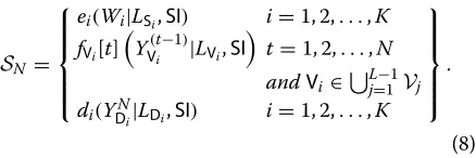
Definition 2A StrategySN is defined as the set of: (1) all encoding functions at the sources, (2) all decoding func-tions at the destinafunc-tions, and (3) the relay strategy for t=1, 2,. . .,N, i.e., for all network states consistent with the side information.
Moreover, for S-D pairi, we denote the maximum achiev-able rate with full network knowledge by Ci. The sum capacityCsum is the supremum ofKi=1Ri over all pos-sible encoding and decoding functions with full network knowledge.
We now define the normalized sum rate and the nor-malized sum capacity.
Definition 3([2])Normalized sum rate ofαis said to be achievable if there exists a set of strategies{Sj}Nj=1such that following holds. As N goes to infinity, strategySN yields a sequence of codes having rates Riat sourceSi, i=1,. . .,K , go to zero for all the network states consistent with the side information and for a constantτthat is independent of the channel gains.
Definition 4 ([2])Normalized sum capacity α∗ is defined as the supremum of all achievable normalized sum ratesα. Note thatα∗∈[ 0, 1].
Remark 2While the results of this paper may appear pessimistic, they are much like any other compound chan-nel analysis which aims to optimize the worst case scenario. We adopted the normalized capacity as our metric which opens the door for exact (or near-exact) results for several cases as we will see in this paper. We view our current formulation as a step towards the general case, much like the commonly accepted methodology where channel state information is assumed known perfectly in first steps of a new problem (MIMO, interference channels, scaling laws), even though that assumption is almost never possible.
3 Motivating examples
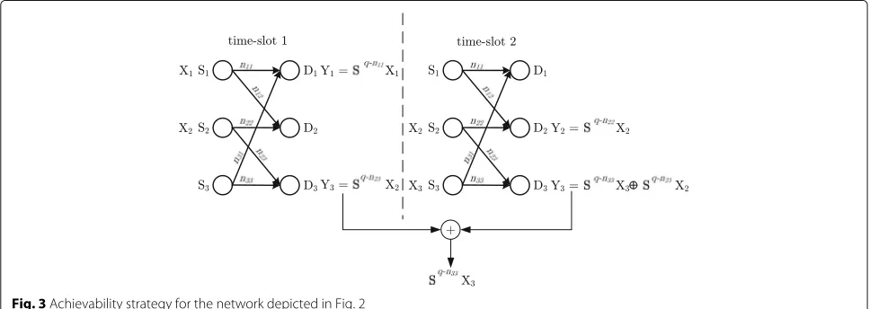
Before diving into the main results, we use a sequence of examples to understand the mechanisms that allow us outperform interference avoidance with only 1-local view. We first consider the single-layer network depicted in Fig. 2a. Using interference avoidance, we can create the induced subgraphs of all three S-D pairs as shown in Fig. 2b in three time slots. Thus, with interference avoid-ance, one can only achieveα = 13 which is the same as TDMA. However, we show that it is possible to recon-struct the three induced subgraphs in only two time slots and to achieveα= 12with 1-local view.
a
b
Fig. 2 aA network in which coding is required to achieve the normalized sum capacity andbthe induced subgraphs
original network by using only two time slots such that all nodes receive the same signal as if they were in the induced subgraphs. This would immediately imply that a normalized sum rate of12is achievable1.
To do so, we split the communication block into two time slots of equal length. Sources S1 and S2 transmit
the same codewords as if they are in the induced sub-graphs over first time slot. Destination D1 receives the
same signal as it would have in its induced subgraph, and destinationD3receives interference from sourceS2.
Over second time slot,S3transmits the same codeword
as if it was in its induced subgraph and S2 repeats its
transmit signal from the first time slot. Destination D2
receives its signal interference-free. Now, if destination D3 adds its received signals over the two time slots, it
recovers its intended signal as depicted in Fig. 3. In other words, we used interference cancellation at destination D3. Therefore, all S-D pairs can effectively communicate
interference-free over two time slots.
We can view this discussion in an algebraic framework. To each sourceSi, we assign a transmit vectorTSi of size 2×1 where 2 corresponds to the number of time slots. If the entry at rowtis equal to 1, thenSicommunicates the
codeword forDiduring time slott,i=1, 2, 3, andt=1, 2. In our example, we have
TS1 =
1 0
, TS2 =
1 1
, TS3 =
0 1
. (9)
To each destinationDi, we assign a receive matrixRDi of size 2×2 where each row corresponds to a time slot and each column corresponds to a source that has a route to destinationDi. More precisely,RDi is formed by con-catenating the transmit vectors of the sources that are connected toDi. In our example, we have
RD1 =
TS1TS3
= t=1 t=2
S1 S3
1 0 0 1
, (10)
RD2 = t=1
t=2
S1 S2
1 1 0 1
, RD3 = t=1
t=2 S2 S3
1 0 1 1
.
From the receive matrices in (10), we can easily check whether each destination can recover its corresponding signal or not. For instance, fromRD1, we know that in time
slot 1, the signal fromS1is received interference-free. A
similar story is true for the second pair andRD2. FromRD3,
we see that in time slot 2, the signal fromS3is received
with interference from S2. However, with a linear
row-operation, we can create a row where the only 1 appears in the column associated withS3. More precisely,
RD3(1, :)⊕RD3(2, :)=
S2 S3
(0 1).
whereRD3(t, :)denotes rowtof matrixRD3. Thus, each destination can recover its intended signal interference-free over two time slots. More precisely, we require
Si Sj
(1 0)∈rowspanRDi
, i,j∈ {1, 2, 3}, j=i. (11)
This example illustrated that with only 1-local view, it is possible to reconstruct the three induced subgraphs in only two time slots using (repetition) coding at the sources and go beyond interference avoidance and TDMA. In the following example, we show that more sophisticated ideas are required to beat TDMA in multi-layer networks.
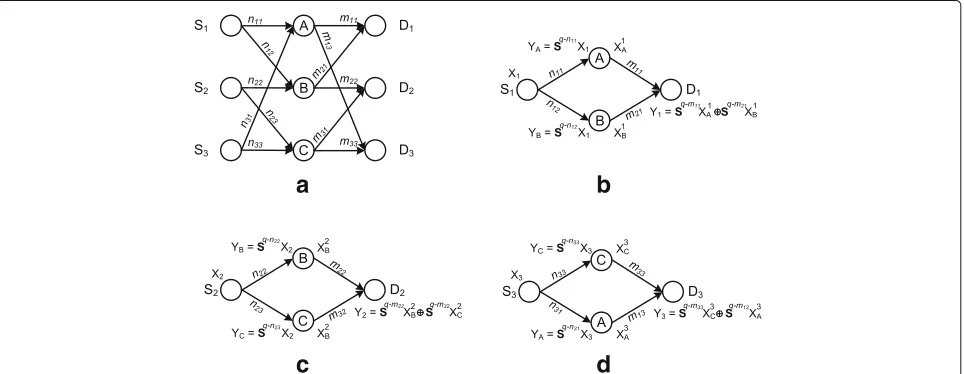
Consider the two-layer network of Fig. 4a. Under the lin-ear deterministic model it is straightforward to see that by using interference avoidance or TDMA, it takes three time slots to reconstruct the induced subgraphs of Fig. 4b–d, which results in a normalized sum rate ofα= 13.
We now show that using repetition coding at the sources and linear coding at the relays, it is possible to achieveα= 1/2 and reconstruct the three induced subgraphs in only two time slots. This example was first presented in [1].
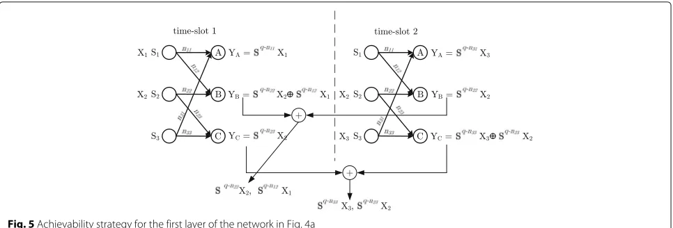
Consider any strategy for S-D pairs 1, 2, and 3 as illus-trated in Fig. 4b–d. In the first layer, we implement the achievability strategy of Fig. 3 illustrated in Fig. 5. As it can be seen in this figure, at the end of the second time slot, each relay has access to the same received signal as if it was in the diamond networks of Fig. 4b–d.
In the second layer during the first time slot, relaysV1
and V2 transmit XV11 and X1V2, respectively, whereas V3
transmitsXV23 ⊕XV33 as depicted in Fig. 6. DestinationD1
receives the same signal as Fig. 4b. During the second time slot , relaysV2andV3transmitXV22andX
receives the same signal as Fig. 4c. If destinationD3adds
its received signals over the two time slots, it recovers the same signal as Fig. 4d. Therefore, each destination receives the same signal as if it was only in its corresponding dia-mond network over two time slots. Hence, a normalized sum rate ofα= 12is achievable.
Again, this strategy can be viewed in an algebraic frame-work. We assign a transmit vector TSi of size 2×1 to 2×2 where each row corresponds to a time slot, and each column corresponds to a source that has a route to that relay.RVjis formed by concatenating the transmit vectors of the sources that are connected toVj. In our example, we have
From the receive matrices in (14), we can easily check whether each relay has access to the same received signals as if it was in the diamond networks of Fig. 4b–d.
Fig. 5Achievability strategy for the first layer of the network in Fig. 4a
We also assign a transmit matrix TVj of size 2×2 to relayVj where each column corresponds to a S-D pairi such thatVj ∈ Gii. If the entry at rowtand columnSi of this transmit matrixTVjis equal to 1, then the relay com-municates the signal it has for S-D pairiat timet. In our example, we have
TV1 =
t=1
t=2
S1 S3
1 0 1 1
, TV2 =
t=1
t=2
S1 S2
1 0 0 1
,
TV3 = t=1
t=2
S2 S3
1 1 1 0
. (14)
If in rowtmore than one 1 appears, then the relay cre-ates the linear combination of the signals it has for the S-D pairs that have a 1 in their column and transmits it. For instance, relayV1during time slot 2 transmitsXV11⊕X
3
V1.
To each destinationDi, we assign a received matrixRDi of size 2×4 where each row corresponds to a time slot, and each column corresponds to a route from a source through a specific relay (e.g.,S1:V1). In fact,RDiis formed
by concatenating (and reordering columns of ) the trans-mit matrices of the relays that are connected toDi. In our example, we have
RD1 = t=1
t=2
S1:V1 S1:V2 S2:V2 S3:V1
1 1 0 0
1 0 1 1
,
RD2 =
t=1
t=2
S1:V2 S2:V2 S2:V3 S3:V3
1 0 1 1
0 1 1 0
,
RD3 =
t=1
t=2
S1:V2 S2:V2 S2:V3 S3:V3
1 1 0 1
1 1 1 0
. (15)
From the receive matrices in (15), we can verify whether each destination can recover its corresponding signals or not. For instance, fromRD1, we know that in time slot 1,
the signals fromS1through relaysV1andV2are received
interference-free. FromRD3, we see that at each time slot,
one of the two signals thatD3is interested in is received.
However, with a linear row operation, we can create a row where 1s only appear in the columns associated withS3.
More precisely,
Thus, each destination can recover its intended signal interference-free and a normalized sum rate ofα = 12 is achievable.
4 An algebraic framework
In this section, given T ∈ N, we define a set of condi-tions that if satisfied, all induced subgraphs can be recon-structed in T time slots. Consider a two-layer wireless networkG=(V,E,{wij}(i,j)∈E)withKsource-destination
pairs and|V| −2K relay nodes. We label the sources as S1,. . .,SK, the destinations asD1,. . .,DK, and the relays asV1,. . .,V|V|−2K. We also need the following definitions:
Definition 5 We assign a number NVjto relayVjdefined
as
NVj
=i|Vj∈Gii, (17)
and we assign a number NDj to destinationDjdefined as
NDj
In this section, we assign matrices to each node inGand the only difference between the linear deterministic model and the Gaussian model is the entries to these matrices:
1. For the linear deterministic model, all entries to these matrices are in binary field (i.e., either 0 or 1); 2. For the Gaussian model, all entries to these matrices
are in{−1, 0, 1}.
We now describe the assignment of the matrices. Fix
T ∈N.
• We assign a transmit vectorTSiof sizeT×1to
sourceSiwhere each row corresponds to a time slot. • To each relayVj, we assign a receive matrixRVjof
sizeT×din(Vj), and we label each column with a source that has a route to that relay. The entry at row t and column labeled bySiinRVjis equal to the entry
at rowt ofTSi.
• We assign a transmit matrixTVjof sizeT×NVjto
each relay where each column corresponds to a S-D pairi where the relay belongs toGii.
• Finally, to each destinationDi, we assign a receive matrixRDiof sizeT×NDiwhere each column
corresponds to a route from a sourceSjthrough a specific relayVjand is labeled asSj:Vj. The entry at rowt and column labeled bySj:Vj inRDiis equal to
the entry at rowt and column labeled bySjofTVj.
An assignment of transmit and receive matrices to the nodes in the network isvalid if the following conditions are satisfied:
C.1Fori=1, 2,. . .,K:
RankTSi
=1. (19)
C.2For any relayVj, using linear row operationsRVjcan be transformed into a matrix in which ifVj ∈ Gii, then ∃such that all entries in roware zeros except for the column corresponding to sourceSi.
C.3For destinationDi, using linear row operationsRDi can be transformed into a matrix in which∃such that thethrow has only 1s in the columns corresponding to sourceSi,i=1, 2,. . .,K.
Remark 3It is straightforward to show that a neces-sary condition for C.3 is for each TVj to have full
col-umn rank. This gives us a lower bound on T which is
maxVji|Vj∈Gii. Moreover, TDMA is always a lower
bound on the performance of any strategy and thus pro-vides us with an upper bound on T. In other words, we have
max Vj
i|Vj∈Gii≤T <K. (20)
Theorem 1For a K-user two-layer network G =
(V,E,{wij}(i,j)∈E)with 1-local view if there exists a valid assignment of transmit and receive matrices, then all induced subgraphs can be reconstructed in T time slots and a normalized sum rate ofα= T1 is achievable.
Proof We first prove the theorem for the linear deter-ministic model, and then, we provide the proof for the Gaussian model.
Network G hasK S-D pairs. Consider theK-induced subgraphs of all S-D pairs, i.e., Gjj, j = 1, 2,. . .,K. We show that any transmission snapshot over these induced subgraphs can be implemented inGoverTtime slots such that all nodes receive the same signal as if they were in their corresponding induced subgraphs.
Linear deterministic model.Consider a transmission snapshot in theK-induced subgraphs in which:
• NodeVi(similarly a source) in the induced subgraph GjjtransmitsXjVi,
• NodeVi(similarly a destination) in the induced subgraphGjjreceives
YVji= i:(i,i)∈E
Sq−niiXj
Transmission strategy.At any time slott:
• SourceSitransmits
XSi[t]=TSi(t)X
i
Si, (22)
• Each relayVjtransmits
XVj[t]=
Note that condition C.1 guarantees that each source transmits its signal at least once. At any time instanttrelay Vi(similarly a destination) receives
YVi[t]=
i:(i,i)∈E
Sq−niiXV
i[t], t=1,. . .,T, (24)
where summation is performed inFq2.
Reconstructing the received signals. Based on the transmission strategy described above, we need to show that at any nodeVireceived signalYVjican be obtained.
ConditionC.2guarantees that using linear row opera-tions, RVj can be transformed into a matrix in which if Vi ∈ Gjj, then∃such that all entries in roware zeros except for the column corresponding to sourceSj. Note that linear operation in the linear deterministic model is simply the XOR operation. We note that two 1s in the same column of a receive matrix represent the same sig-nals and the same channel gains. Thus,Viis able to cancel out all interference by appropriately summing the received signals at different time slots.
Similar argument holds for any destinationDi. However, since it is possible that there exist multiple routes fromSi toDi, more than a single 1 might be required after the row operations. In fact, condition C.3guarantees that using linear row operations, destination Di can cancel out all interfering signals and only observe the intended signals fromSi.
Gaussian model.The proof presented above holds for the Gaussian channel model with some modifications. First, the operations should be in real domain and the row operations are now either summation or subtraction. At any time slottrelayVjtransmits:
XVj[t]=
Moreover, we need to show that with the row operations performed on received and transmit signals, the capacity of the reconstructed induced subgraphs is “close” to the
capacity of the induced subgraphs when there is no inter-ference. The following lemma shows that the capacity of the reconstructed induced subgraphs is within a constant number of bits of the capacity of the induced subgraphs with no interference. This constant is independent of the channel gains and transmit powerP.
Lemma 1Consider a multi-hop complex Gaussian relay network with one source Sand one destination D repre-sented by a directed graph
G=(V,E,{hij}(i,j)∈E)
where {hij}(i,j)∈E represents the channel gains associated with the edges.
We assume that at each receive node the additive white complex Gaussian noise has variance σ2. We also assume a power constraint of P at all nodes, i.e.,
limn→∞1nEnt=1|XVi[t]|2
≤ P. Denote the capacity of this network by C(σ2,P). Then, for all T ≥ 1, T ∈ R, we have
C(σ2,P)−τ ≤C(Tσ2,P/T)≤C(σ2,P), (26)
whereτ = |V|2 logT+17is a constant independent of the channel gains, P, andσ2.
ProofFirst note that by increasing noise variances and by decreasing the power constraint, we only decrease the capacity. Hence, we have C(Tσ2,P/T) ≤ C(σ2,P). To prove the other inequality, we use the results in [28]. The cut-set boundC¯ is defined as
¯
the cut-set bound evaluated for i.i.d.N(0,P)input distri-butions, andGis the transfer matrix associated with the cut, i.e., the matrix relating the vector of all the inputs at the nodes in, denoted byX, to the vector of all the
where |V| is the total number of nodes in the network. Similarly, we have
¯
Ci.i.d(Tσ2,P/T)−15|V| ≤C(Tσ2,P/T)
C(Tσ2,P/T)≤ ¯Ci.i.d(Tσ2,P/T)+2|V|. (29)
Now, we will show that
For any S-D cut, ∈ D, σP2GG∗is a positive
semi-definite matrix. Hence, there exists a unitary matrix U
such thatUGdiagU∗= σP2GG∗whereGdiagis a diagonal matrix. Refer to the non-zero elements inGdiagasgii’s. We have:
cally increasing ingii.
Now suppose that min∈ Dlog|I+T2Pσ2GG∗| =
where (a) follows from (31). From (28) and (29), we have
C(σ2,P)−C(Tσ2,P/T)≤ min
where(a)follows from (32). Therefore, we get
C(σ2,P)−τ ≤C(Tσ2,P/T)≤C(σ2,P), (34)
whereτ = |V|2 logT+17is a constant independent of the channel gains,P, andσ2.
5 Optimality of the strategies
In this section, we consider several classes of networks and derive the minimum number of time slots such that all induced subgraphs can be reconstructed as if there is no interference present. In other words, we characterize the normalized sum capacity of such networks.
5.1 Single-layer folded-chain networks
We start by considering a single-layer network motivated by the downlink cellular system similar to the one in Fig. 7.
Definition 6 A single-layer (K,m) folded-chain (1 ≤
m≤K ) network is a single-layer network with K S-D pairs. In this network, sourceSiis connected to destinations with ID’s1+{(i−1)++(j−1)}modKwhere i = 1,. . .,K , j=1,. . .,m and(i−1)+=max{(i−1), 0}.
Figure 8 is the single-layer(3, 2)folded-chain network corresponding to the downlink cellular system of Fig. 7. The following theorem characterizes the normalized sum capacity of such networks.
Theorem 2The normalized sum capacity of a single-layer (K,m) folded-chain network with 1-local view is
α∗= 1
m.
To achieve the normalized sum capacity of a single-layer(K,m)folded-chain network with 1-local, we need to incorporate repetition coding at the sources. We note that a single-layer(K,K)folded-chain network is aKuser fully connected interference channel, and in that case, with
Fig. 8The corresponding networkGfor the downlink cellular system illustrated in Fig. 7
1-local view, interference avoidance achieves the normal-ized sum capacity of 1/K.
ProofAchievability: We provide a valid assignment of transmit and receive matrices to the nodes withT = m. Then, by Theorem 1, we know that a normalized sum rate ofm1 is achievable.
Supposem < K < 2m (we will later generalize the achievability scheme for arbitraryK), letm =K−m. To each sourceSi,i = 1,. . .,K, we assign a transmit vector
TSisuch that:
TSi(j)=1⇔j≤i≤j+m, j=1,. . .,m. (35)
Remark 4For single-layer folded-chain networks, the assignment of the transmit vectors in (35) is the same for the linear deterministic model and the Gaussian model.
This assignment satisfies conditionsC.1-C.3:
• C.1is trivially satisfied since for any sourceSi, there exists at least one value ofj such thatTSi(j)=1.
• C.2is irrelevant since we have a single-layer network, and no relay is present.
• C.3is satisfied since for1≤i≤m,RDihas a single 1
in rowi and the column labeled asSi, and for m<i<2m, the summation of rows
i−m+1,. . .,i−1,iofRDihas a single 1 in the
column labeled asSi.
Since conditionsC.1-C.3are satisfied, from Theorem 1, we know that we can achieveα= m1.
For generalK, the achievability works as follows. Sup-pose,K=c(2m−1)+r, wherec≥1 and 0≤r< (2m−1), we implement the scheme for S-D pairs 1, 2,. . ., 2m−1 as if they are the only pairs in the network. The same for source-destination pairs 2m, 2m+1,. . ., 4m−2, etc. Finally, for the lastrS-D pairs, we implement the scheme withm=max{r−m+1, 1}. This completes the proof of achievability.
Converse: Assume that a normalized sum rate ofα is achievable3. We show thatα≤ 1
m. Consider a single-layer (K,m)folded-chain network in which the channel gain of a link fromSito destinationsi,i+1,. . .,mis equal ton∈ N(for the linear deterministic model) andh∈C(for the Gaussian model),i = 1, 2,. . .,m, and all other channel gains are equal to zero. See Fig. 9 for a depiction.
Destination Dm after decoding and removing the con-tribution ofSmhas the same observation (up to the noise term) asDm−1. Thus,Dmis able to decode Wm−1. With a
recursive argument, we conclude that
n
⎛ ⎝
j=1,2,...,m Rj−n
⎞
⎠≤HYmn|LDm,SI
. (36)
The MAC capacity at destinationDmin the linear deter-ministic model gives us
m(αn−τ)≤n⇒(mα−1)n≤dτ. (37)
Since this has to hold for all values ofn, andαandτare independent ofn, we getα ≤ m1. For the Gaussian model, the MAC capacity atDmgives us
m(αlog(1+ |h|2)−τ)≤log(1+m× |h|2), (38)
which results in
(mα−1)log(1+ |h|2)≤log(m)+mτ. (39)
Since this has to hold for all values ofh, andαandτare independent ofh, we getα≤ m1. This completes the proof of Theorem 2.
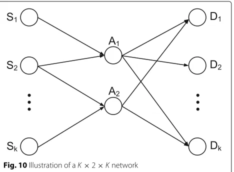
5.2 K×2×Knetworks
We move to two-layer networks and start with a special class of networks defined below.
Definition 7A K×2×K network is a two-layer network (as defined in Section2.1) with|V| −2K=2.
We establish the normalized sum capacity of such net-works in the following theorem.
Theorem 3 The normalized sum capacity of a K×2×K network with 1-local view isα∗ = 1/dmaxwhere dmaxis
defined in (7).
ProofThe result forK =1 is trivial, so we assumeK >
1. We refer to the two relays asA1andA2, see Fig. 10.
Achievability: We divide the S-D pair IDs into three disjoint subsets as follows:
• Jiis the set of all the S-D pair IDs such that the corresponding source is connectedonly to relayAi, i=1, 2;
Fig. 10Illustration of aK×2×Knetwork
• J12is the set of all the other S-D pair IDs. In other
words,J12is the set of all the S-D pair IDs where the
corresponding source is connected to both relays.
Without loss of generality assume that din(A2) ≥
din(A1)and rearrange sources such that
J1= {1, 2,. . .,din(A1)},
J2= {din(A1)+1,. . .,din(A1)+din(A2)},
J12= {din(A1)+din(A2)+1,. . .,K}. (40)
We pick the smallest member of J1 and the smallest
member of J2, and we set the first entry of the
corre-sponding transmit vectors equal to 1 and all other entries equal to zero. We remove these members from J1 and
J2. Then, we pick two smallest members of (updated)J1
andJ2and we set the second entry of the corresponding
transmit vectors equal to 1 and all other entries equal to zero. We continue this process untilJ1is empty. For any
remaining S-D pair IDj, we set thejth entry of the corre-sponding transmit vector equal to 1 and all other entries equal to zero.
In the second layer, we divide S-D pair IDs based on the connection of destinations to relays, i.e.,Jiis the set of all the S-D pair IDs such that the corresponding des-tination is connected to relayAi,i = 1, 2, andJ12 is the
set of all the other S-D pair IDs. ToAi, we assign a trans-mit matrix of sizeT ×Ji+J12 ,i = 1, 2, as described below.
Without loss of generality assume that dout(A2) ≥
dout(A1). We pick one member of J1 and one member
ofJ2 randomly, and in the first row ofTA1 andTA2, we
then pick one member of (updated)J1 and one member of (updated)J2randomly, and in the second row ofTA1
andTA2, we set the entry at the column corresponding to
the picked indices equal to 1 and all other entries in those rows equal to zero. We continue this process untilJ1 is empty.
We then pick one of the remaining S-D pair IDs (mem-bers ofJ12 and the remaining members ofJ2), and we assign a 1 in the next available row and to the column corresponding to the picked index in the corresponding transmit matrix. We set all other entries in those rows equal to zero. We continue the process until no S-D pair ID is left.
Condition C.1 is trivially satisfied. The correspond-ing transmission strategy in this case would be a “per layer” interference avoidance, i.e., if in the first hop, two sources are connected to the same relay, they do not transmit simultaneously, and if in the second hop, two destinations are connected to the same relay, they are not going to be served simultaneously. There-fore, since the scheme does not allow any interfer-ence to be created, no row operations on the receive matrix is required and conditions C.2 and C.3 are satisfied.
Note that according to the assignment of the vectors and matrices, we require
T =max{din(A2),dout(A2)} =dmax. (41)
Hence, from Theorem 1, we know that a normalized sum rate ofα= d1
max is achievable.
Remark 5For K×2×K networks, the assignment of the transmit vectors and matrices is the same for the linear deterministic model and the Gaussian model.
Converse: Assume that a normalized sum rate of α is achievable, we show that α ≤ d1
max. It is
suffi-cient to consider two cases: (1) dmax = din(A1) and
(2) dmax = dout(A1). Here, we provide the proof for
case (1) and we postpone the proof for case (2) to Appendix B.
The proof is based on finding a worst-case scenario. Thus, to derive the upper bound, we use specific assign-ment of channel gains. ConsiderDjforj ∈ J1, any such
destination is either connected to relay A1 or to both
relays. If it is connected to both, then set the channel gain from relayA2equal to 0. Follow similar steps for the
members ofJ2.
Now, considerDjforj∈ J12, such destination is either
connected to only one relay or to both relays. If such destination is connected to both relays, assign the channel
gain of 0 to one of the links connecting it to a relay (pick this link at random).
For all other links in the network, assign a channel gain ofn∈N(in the linear deterministic model) andh∈C(in the Gaussian model). With this channel gain assignment, we have:
∀j ∈ J1: HWj|YAn1,LA1,SI≤nn, (42) wheren→0 asn→ ∞. Thus, relayA1is able to decode
all messages coming from sources corresponding to the members ofJ1.
A similar claim holds for relay A2 and all messages
coming from J2. Relays A1 and A2 decode the
mes-sages coming from members ofJ1andJ2, respectively,
and remove their contributions from the received signals. After removing the contributions from members of J1
andJ2, relayA1can decode the message of members in
J12, i.e.,
Thus, each relay is able to decode the rest of the mes-sages (in the linear deterministic case, relays have the same received signals and in the Gaussian case, they receive the same codewords with different noise terms). This means that relayA1is able to decode all the messages
fromJ1andJ12, i.e.,
which in turn implies that
n
Given the assumption of 1-local view, in order to achieve a normalized sum rate ofα, each source should transmit at a rate greater than or equal toαn−τ (in linear deter-ministic model) for some constantτ. This is due to the fact that from each source’s point of view, it is possible that the other S-D pairs have capacity 0. Therefore, in order to achieve a normalized sum rate ofα, it should transmit at a rate of at leastαn−τ. The MAC capacity at relayA1
gives us
din(A1)(αn−τ)≤n⇒(din(A1)α−1)n≤din(A1)τ.
Since this has to hold for all values ofn, andα andτ are independent ofn, we getα ≤d 1
in(A1).
In the Gaussian case, each source should transmit at a rate greater than or equal toαlog(1+ |h|2)−τsince from each source’s point of view, it is possible that the other S-D pairs have capacity 0. From the MAC capacity at relay A1, we get
din(A1)
αlog(1+ |h|2)−τ≤log1+din(A1)× |h|2
, (47)
which results in
din(A1)
αlog1+ |h|2−τ≤log(din(A1))+log
1+×|h|2. (48)
Hence, we have
(din(A1)α−1)log(1+ |h|2)≤log(din(A1))+din(A1)τ.
(49)
Since this has to hold for all values ofh, andα andτ are independent ofh, we getα≤ d 1
in(A1).
Combining the argument presented above with the result in Appendix B, we get
α≤ 1 dmax
. (50)
This completes the proof of the converse.
5.3 3×3×3 networks
In this subsection, we consider two-layer networks with three source-destination pairs and three relays. We face networks in which we need to incorporatenetwork cod-ing techniques to achieve the normalized sum capacity with 1-local view. The coding comes in the form of rep-etition coding at sources and a combination of reprep-etition and network coding at relays.
Definition 8 A3×3×3network is a two-layer network (as defined in Section2.1) with K=3and|V| −2K=3.
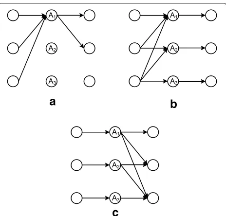
Theorem 4The normalized sum capacity of a3×3×3
network with 1 local view,α∗is equal to
1. 1 if and only ifGii∩Gjj= ∅fori=j.
2. 1/3if and only if one of the graphs in Fig. 11 is a subgraph of the network connectivity graphG. 3. 1/2otherwise.
Fig. 11 a–cThe normalized sum capacity of a 3×3×3 network with 1-local view,α∗, is equal to 1/3 if and only if one of the graphs in this figure is a subgraph ofG
As we show in this section, the transmission strategy is a combination of three main techniques:
1. Per layer interference avoidance
2. Repetition coding to allow overhearing of the interference
3. Network coding to allow interference neutralization
Remark 6From Theorems3and4, we conclude that for all single-layer, K×2×K , and3×3×3networks with 1-local view, the normalized sum capacityα∗= 1/K (i.e., TDMA) is optimal if and only if when all channel gains are equal and non-zero, then there exists a node that can decode all messages. We refer to such node as an “omni-scient” node. We believe this observation holds for much more general network connectivities with 1-local view or in fading networks with no channel state information at the transmitters. However, this is a different line of research and it is beyond the scope of this paper. Omniscient nodes are studied in [29, 30]in the context of source two-destination multi-layer wireless networks where they dic-tate the asymptotic (in terms of power) behavior of these networks.
Suppose none of the graphs in Fig. 11 is a subgraph of Gand that the network does not fall in category (a). This immediately impliesdmax=2.
We have the following claim for such networks.
ClaimFor a 3 × 3× 3 network with dmax = 2, the
only connectivity that results in a per layer fully connected conflict graph is the one shown in Fig.12.
If the per layer conflict graphs are not fully con-nected and the network does not fall in category (a), then a normalized sum rate of α = 1/2 is eas-ily achievable. Moreover, from claim 1, we know that with dmax = 2, the folded-chain structure of Fig. 12
exists in at least one of the layers. In Section 3, we showed that a normalized sum rate of α = 1/2 is achievable.
We note that these cases can be easily described within the algebraic framework of Section 4. In fact, if the
folded-Fig. 12The only connectivity that results in a per layer fully connected conflict graph in a 3×3×3 network withdmax=2
chain structure of Fig. 12 exists in at least one of the layers, as shown in Section 3, the transmission can be expressed as a valid assignment of transmit and receive matrices. However, if the per layer conflict graphs are not fully connected and the network does not fall in category (a), then the scheme is a per layer interfer-ence avoidance which can be easily expressed in terms of a valid assignment of transmit and receive matrices. Finally, we note that for all 3 × 3 × 3 networks, the assignment of the transmit vectors and matrices is the same for the linear deterministic model and the Gaussian model.
Converse:The forward direction of the proof for net-works in category (a) is trivial as there is no interference present in such networks. For the reverse direction as shown in Lemma 3 Appendix A, for any network that does not fall into category (a), an upper bound of 1/2 on the normalized sum capacity holds. Moreover, Lemma 3 also provides the outer-bound for networks in category (c). Thus, we only need to consider 3× 3× 3 networks in category (b).
For 3 × 3 × 3 networks in category (b), we first consider the forward direction. One of the graphs in Fig. 11 is a subgraph of the network connectivity graph G, say the graph in Fig. 11b. Assign channel gain of
n ∈ N(in linear deterministic model) and h ∈ C (in Gaussian model) to the links of the subgraph and chan-nel gain of 0 to the links that are not in the graph of Fig. 11b.
With this assignment of the channel gains, we have
HWi|YAni,LAi,SI
≤nn, i=1, 2, 3. (51)
Basically, each destination Di isonlyconnected to relay Ai, and each relay Ai has all the information that des-tination Di requires in order to decode its message, i = 1, 2, 3. Thus, relay A1 can decode W1. After
removing the contribution of S1, relay A1 is able to
decode W2. Continuing this argument, we conclude
that
n
⎛ ⎝3
j=1
Rj−n ⎞
⎠≤HYAn1|LA1,SI
. (52)
The MAC capacity at relayA1, for the linear
determin-istic model, gives us
3(αn−τ)≤n⇒(3α−1)n≤dτ. (53)
3(αlog(1+ |h|2)−τ)≤log(1+3× |h|2), (54)
which results in
(3α−1)log(1+ |h|2)≤log(3)+3τ. (55)
Since this has to hold for all values ofh, andα andτ are independent ofh, we getα≤ 13. The proof for the graphs in Fig. 11a, c is very similar.
For the reverse direction, if none of the graphs in Fig. 11 is a subgraph of the network connectivity graphG, a nor-malized sum rate ofα= 12is achievable and optimal. This completes the converse proof.
5.4 Folded-chain networks
We now consider a class of networks for which we need to incorporate network coding in order to achieve the normalized sum capacity with 1-local view. This class is the generalization of the networks in Section 5.1 to two layers.
Definition 9A two-layer(K,m) folded-chain network (1 ≤ m ≤ K ) is a two-layer network with K S-D pairs and K relays in the middle. Each S-S-D pair i has m disjoint paths, through relays with indices 1 +
{(i−1)++(j−1)}modK where i = 1,. . .,K , j =
1,. . .,m.
Theorem 5 The normalized sum capacity of a two-layer
(K,m)folded-chain network with 1-local view isα∗= m1.
ProofAchievability: The result is trivial form=1. For
m = K, the upper bound of α = K1 can be achieved simply by using TDMA. Similar to Theorem 2, suppose
m < K < 2m. The extension to the general case would be similar to Theorem 2. Here, we describe how to construct a valid assignment of transmit and receive matrices.
The assignment of the transmit vectors in the first layer is identical to that of Theorem 2 as given in (35). We note that each relay can recover all incoming sig-nals with this assignment. For the second layer, we have
K+1 steps.
•Steps 1 throughm: Our goal is to provide destination Di, 1 ≤ i ≤ m, during time sloti with its desired sig-nal without any interference. Therefore, rowiof any relay
connected toDi has a single 1 in the column associated with S-D pairiand 0s elsewhere;
•Stepsm+1 throughK: During stepi,m+1≤i≤K, our goal is to provide destinationDiwith its desired signal (interference will be handled later). To do so, consider the transmit matrix of any relay connected tosfDi; and place a single 1 in the column associated with S-D pairiand the row with the smallest index and least number of 1s;
• StepK + 1: During this step, our goal is to resolve interference and goes through the following loop:
1. LetLjdenote the set of row indices for which there exists at least 1 in the column associated with S-D pairj of the transmit matrix of a relay connected to
Dj,m+1≤j≤K;
then make this summation 0 making any of the
TVp
,Sj
’s that is not previously assigned equal to 14;
3. Setj=j+1; Ifj>Kand during the previous loop no change has occurred, then set all entries that are not yet defined equal to zero and terminate; otherwise, go to line 2 of the loop.
We now describe the K + 1 steps via an example of (5, 3)two-layer folded-chain network of Fig. 13. In Fig. 14, we have demonstrated the evolution of the relays’ trans-mit matrices at the end of stepsm,K, andK+1. For this example, the loop in stepK+1 is repeated three times.
It is easy to verify conditionC.3for destinationD1,D2,
andD3. We have providedRD4 in (56), and as we can see,
by adding the first and the second row, we can have a row that has only 1s in the columns corresponding to source S4. Similarly, we can show that the condition holds forD5.
Fig. 13A(5, 3)two-layer folded-chain network
K
i=1
Ri≥αCsum−τ, (58)
with error probabilities going to zero asN → ∞and for some constantτ ∈Rindependent of the channel gains.
Consider the first layer of the two-layer(K,m) folded-chain network, where the channel gain of a link from sourceito relaysi,i+1,. . .,mis equal ton∈N(for the linear deterministic model) andh ∈ C(for the Gaussian model),i = 1, 2,. . .,m, and all the other channel gains are equal to zero. In the second layer, we set the channel gain from relayito destinationiequal ton(for the linear deterministic model) orh(for the Gaussian model), and all other channel gains equal to 0,i=1, 2,. . .,m. See Fig. 15 for a depiction.
With this configuration, each destinationDiisonly con-nected to relayAi, and each relayAihas all the information that destinationDirequires in order to decode its message, i=1,. . .,m. We have
HWi|YAni,LAi,SI
≤nn, i=1,. . .,m. (59)
At relay Am after decoding and removing the contri-bution ofSm, relayAm is able to decode Wm−1. With a
Fig. 15Channel gain assignment in a two-layer(K,m)folded-chain network. Allsolid linkshave capacityn(for the linear deterministic model) andh(for the Gaussian model), and alldashed linkshave capacity 0
recursive argument, we conclude that
n
⎛ ⎝
j=1,2,...,m Rj−n
⎞
⎠≤HYAnm|LAm,SI
. (60)
The MAC capacity at relayAmfor the linear determin-istic model gives us
m(αn−τ)≤n⇒(mα−1)n≤dτ. (61)
Since this has to hold for all values ofn, andα andτ are independent ofn, we getα ≤ m1. For the Gaussian model, the MAC capacity at relayAmgives us
m(αlog(1+ |h|2)−τ)≤log(1+m× |h|2), (62)
which results in
(mα−1)log(1+ |h|2)≤log(m)+mτ. (63) Since this has to hold for all values ofh, andα andτ are independent ofh, we getα≤ m1.
5.5 Gain of coding over interference avoidance: nested folded-chain networks
In this subsection, we show that the gain from using coding over interference avoidance techniques can be unbounded. To do so, we first define the following class of networks.
Definition 10An L-nested folded-chain network is a single-layer network with K = 3L S-D pairs,{S1,. . .,S3L}
and {D1,. . .,D3L}. For L = 1, an L-nested folded-chain
network is the same as a single-layer (3, 2) folded-chain network. For L > 1, an L-nested folded-chain network is formed by first creating three copies of an(L−1)-nested folded-chain network. Then,
• The i-th source in the first copy is connected to the i-th destination in the second copy,i=1,. . ., 3L−1, • The i-th source in the second copy is connected to
the i-th destination in the third copy,i=1,. . ., 3L−1,
• The i-th source in the third copy is connected to the i-th destination in the first copy,i=1,. . ., 3L−1.
Figure16illustrates a 2-nested folded-chain network.
Consider anL-nested folded-chain network. The con-flict graph of this network is fully connected, and as a result, interference avoidance techniques can only achieve a normalized sum rate of13L. However, we know that for a single-layer (3, 2) folded-chain network, a normalized sum rate of 12is achievable.
Hence, applying our scheme to anL-nested folded-chain network, a normalized sum rate of12Lis achievable. For instance, consider the 2-nested folded-chain network in Fig. 16. We show that any transmission strategy over the induced subgraphs can be implemented in the original
network by using only four time slots such that all nodes receive the same signal as if they were in the induced subgraphs.
To achieve a normalized sum rate ofα =122, we split the communication block into four time slots of equal length. During time slot 1, sources 1, 2, 4, and 5 transmit the same codewords as if they are in the induced sub-graphs. During time slot 2, sources 3 and 6 transmit the same codewords as if they are in the induced subgraphs, and sources 2 and 5 repeat their transmit signal from the first time slot. During time slot 3, sources 7 and 8 trans-mit the same codewords as if they are in the induced subgraphs, and sources 4 and 5 repeat their transmit sig-nal from the first time slot. During time slot 4, source 9 transmits the same codewords as if it is in the induced subgraph, and sources 5, 6, and 8 repeat their transmit signal.
It is straightforward to verify that with this scheme, all destinations receive the same signal as if they were in the induced subgraphs. Hence, a normalized sum rate of α =1
2
2
is achievable for the network in Fig. 16. There-fore, the gain of using coding over interference avoidance is32Lwhich goes to infinity asL→ ∞. See Fig.17 for a depiction. As a result, we can state the following lemma.
Lemma 2Consider an L-nested folded-chain network. The gain of using MCL scheduling over MIL scheduling is
3
2
L
which goes to infinity as L→ ∞.
The scheme required to achieve a normalized sum rate of α = 12L for anL-nested folded-chain network can be viewed as a simple extension of the results presented in Section 4. In a sense instead of reconstructing a sin-gle snapshot, we reconstructLsnapshots of the network. The following discussion is just for the completion of the results.
To each sourceSi, we assign a transmit vectorTSiof size (LT)×1 where each row corresponds to a time slot. If we denote the transmit signal of nodeSiin theth snapshot byXS
i, then ifTSi(j)= 1 andcT+1 ≤j< (c+1)Tfor
c=0, 1,. . .,L−1, thenSicommunicatesXcS+i 1. The other transmit and receive matrices can be described similarly. ConditionsC.2andC.3have to be satisfied for submatri-ces ofRVjcorresponding to rowscT+1,cT+2,. . .,(c+ 1)T−1 forc=0, 1,. . .,L−1.
6 Conclusions
In this paper, we studied the fundamental limits of com-munications over multi-layer wireless networks where each node has limited channel state information. We developed a new transmission strategy for multi-layer wireless networks with partial channel state informa-tion (i.e., 1-local view) that combines multiple ideas including interference avoidance and network cod-ing. We established the optimality of our proposed strategy for several classes of networks in terms of achieving the normalized sum capacity. We also demon-strated several connections between network topol-ogy, normalized sum capacity, and the achievability strategies.
So far, we have only studied cases with 1-local view. One major direction is to characterize the increase in normalized sum capacity as nodes learn more and more about the channel state information. We also focused on the case in which wireless nodes know the network connectivity globally, but the actual val-ues of the channel gains are known for a subset of flows. Another important direction would be to under-stand the impact of local connectivity knowledge on the capacity and to develop distributed strategies to
optimally route information with partial connectivity knowledge.
Endnotes
1Since in two time slots, any transmission strategy
for the diamond networks can be implemented in the original network, we can implement the strategies that achieve the capacity for any S-D pair i with full net-work knowledge, i.e., Ci, over two time slots as well. Hence, we can achieve 12(C1+C2+C3). On the other
hand, we have Csum ≤ C1 + C2 + C3. As a result,
we can achieve a set of rates such that 3i=1Ri ≥
1
2Csum, and by the definition of normalized sum rate, we
achieveα = 12.
2A cutis a subset ofV such thatS ∈ ,D∈/ , and
c=V\.
3The result form = 1 is trivial since we basically have
an interference-free network.
Appendix A: Outer-bound of 1/2 for networks with interference
Lemma 3 In a K-user multi-layer network (linear deter-ministic or Gaussian) with 1-local view if there exists a path fromSitoDj, for some i=j, then the normalized sum capacity is upper-bounded byα=1/2.
Proof Consider a path from sourceSito destinationDj, i = j, i,j ∈ {1,. . .,K}. Assign channel gain of n ∈ N
(for the linear deterministic model) and h ∈ C(for the Gaussian model) to all edges in this path. For each one of the two S-D pairsiandj, pick exactly one path from the source to the destination and assign channel gain ofn
(for the linear deterministic model) orh(for the Gaussian model) to all edges in these paths. Assign channel gain of 0 to all remaining edges in the networkG. See Fig. 18 for an illustration.
In order to guarantee a normalized sum rate of α with 1-local view, each source has to transmit at a rate greater than or equal to αn − τ (for the linear deter-ministic model) orαlog(1+ |h|2)−τ (for the Gaussian model). This is due to the fact that from each source’s point of view, it is possible that the other S-D pairs have capacity 0.