R E S E A R C H
Open Access
A new DOA-based factor graph
geolocation technique for detection of
unknown radio wave emitter position using
the first-order Taylor series approximation
Muhammad Reza Kahar Aziz
1,2*, Khoirul Anwar
1and Tad Matsumoto
1,3Abstract
This paper proposes a new geolocation technique to improve the accuracy of the position estimate of a single unknown (anonymous) radio wave emitter. We consider a factor graph (FG)-based geolocation technique, where the input are the samples of direction-of-arrival (DOA) measurement results sent from the sensors. It is shown that the accuracy of the DOA-based FG geolocation algorithm can be improved by introducing approximated expressions for the mean and variance of the tangent and cotangent functions based on the first-order Taylor series (TS) at the tangent factor nodes of the FG. This paper also derives a closed-form expression of the Cramer-Rao lower bound (CRLB) for DOA-based geolocation, where the number of samples is taken into account. The proposed technique does not require high computational complexity because only mean and variance are to be exchanged between the nodes in the FG. It is shown that the position estimation accuracy with the proposed technique outperforms the conventional DOA-based least square (LS) technique and that the achieved root mean square error (RMSE) is very close to the theoretical CRLB.
Keywords: CRLB, DOA, Factor graphs, Geolocation, Taylor series
1 Introduction
Accurate wireless geolocation has received considerable attention in the past two decades [1] and is expected to play important roles in current and future wireless communications systems. This technology is the key to supporting location-based service applications, e.g., Emergency-911 (E-911), location-sensitive billing, smart transportation systems, vehicle navigation, fraud detec-tion, people tracking, and public safety systems [1–3]. This paper proposes a new direction-of-arrival (DOA)-based factor graph (FG) geolocation technique to detect the position of a single unknown anonymous radio wave emitter (the terminology “anonymous” is omitted in the rest of the paper for simplicity), where to convert
*Correspondence: [email protected]
1School of Information Science, Japan Advanced Institute of Science and Technology (JAIST), 1-1 Asahidai, Nomi-shi 923-1292, Japan
2Electrical Enginering Department, Institut Teknologi Sumatera (ITERA), Lampung Selatan 35365, Indonesia
Full list of author information is available at the end of the article
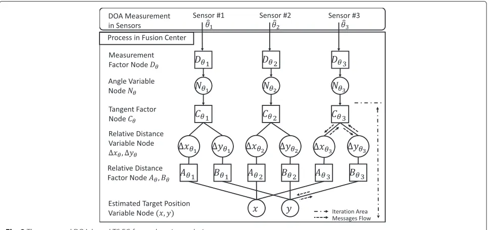
the measured DOA samples to the mean and variance of the tangent and cotangent functions, we utilize the first-order Taylor series (TS) approximation. The proposed technique is not only applicable for an unknown radio wave emitter, e.g., illegal radio wave emitter, but it is also applicable for common radio wave emitter position detec-tion. The basic setup is shown in Fig. 1, where the FG is performed at the fusion center.
The FG is first applied on a geolocation technique in [4]. In the FG, the complexity is reduced because the global function factors into the products of several sim-ple local functions, and the messages passed through the nodes are in the form of mean and variance, because of the Gaussianity assumption of the measured sample dis-tribution [5–8]. The FG technique has been extended to incorporate not only DOA [6, 7] but also other informa-tion sources such as time of arrival (TOA) [8, 9], time difference of arrival (TDOA) [10], and received signal strength (RSS) [11], since the location of the unknown
Fig. 1Basic structure of FG-based unknown radio wave emitter detection describing a single target, four monitoring spots (in the case of RSS-based FG technique), three sensors, and fusion center
radio wave emitter can be estimated from them. In this paper, we use the terminology DOA instead of angle of arrival (AOA) for better expression.
DOA is used in this paper because it is measured by using either antenna arrays or a directional antenna with-out requiring perfect synchronization, time stamp, or transmit power information of a single unknown radio wave emitter [12, 13]. The other FG-based techniques, in contrast to the DOA-based techniques, e.g., TOA-based techniques, should perform perfect time synchronization among the sensors as well as between the sensors and the unknown emitter. The TDOA-based techniques can eliminate the necessity of the synchronization between the sensors and the emitter, but still, the sensors have to be accurately synchronized. Perfect synchronization is needed both in TOA and TDOA because the high velocity of the light, e.g., error of 1μs, leads to error around 300 m [8]. Another difficulty arises in TOA-based geolocation techniques, where the TOA parameters cannot be mea-sured from an unknown radio wave emitter because the time stamp information (time of departure (TOD) of the signal) of the transmitted signal from an unknown radio emitter is not available.
On the other hand, the major difficulty with the RSS-based technique is that it requires equal transmit power between the target and the test signal transmit-ted from the monitoring spots to gather the prelimi-nary RSS map [11]. However, the transmit power of an unknown radio wave emitter is not available. The facts described above motivate us to use the DOA-based FG techniques to detect the position of the unknown radio emitter. The DOA-based FG techniques are also suit-able in line-of-sight (LOS) and imperfect synchronization conditions.
1.1 Related work
A lot of work in DOA-based geolocation techniques have been proposed even since 30 years ago [14, 15]. How-ever, it is quite recently that the FG-based techniques using DOA, TOA, TDOA, and RSS information were proposed, where the measurement data related to those parameters are used as the input to the algorithms. A joint TOA-DOA-based FG geolocation algorithm was proposed in [6], where the measured samples are effi-ciently used in FG to estimate the position accurately. Nevertheless, the joint TOA-DOA-based FG geoloca-tion algorithm shown in [6] is still not fully correct because the message to be exchanged, the information of measurement error derived from the measurement results, enters the FG at an improper node as identified by [8].
The FG geolocation technique derived in [6] is improved in [7] as suggested in [8]. It also removes the necessity of measuring the TOA data from the joint TOA-DOA-based FG geolocation algorithm shown in [6] to obtain a simple DOA-based FG technique. After the DOA-based FG technique reaches a convergence point, the position estimate results are used as the initial posi-tion for the Gauss-Newton (GN) algorithm as the second step of the algorithm, the so-called factor graph-Gauss-Newton (FG-GN) geolocation technique in [7], to attain even higher accuracy.
We found that (1) The distance (r) is used in [7] as
an argument of the tangent and cotangent functions, i.e., tan(r) and cot(r), which is obviously incorrect. Instead, the angle should be the argument of the tangent and cotangent functions, i.e., tan(θ)and cot(θ). (2) The fac-tor node for collecting the samples is not available in the DOA-based FG geolocation techniques in [6, 7]. More-over, the input parameter in [7] isrinstead ofθ. (3) The mean formula of tangent and cotangent function nodes [7] is not clearly described.
The Cramer-Rao lower bound (CRLB) is derived in [7], and the results of a series of simulations conducted to evaluate the accuracy of the DOA-based FG geoloca-tion technique are shown also in [7] for the comparison purpose between CRLB and the root mean square error (RMSE) of DOA-based geolocation techniques, i.e., FG-GN, FG-GN, and FG. However, the CRLB of the DOA-based technique shown in [7] does not take into account the influence of the sample number, and hence, the accuracy of the detection, when the number of the samples is large, is better than the CRLB, leading to the unusefulness of the comparison.
1.2 Contributions
of the DOA samples are used in the FG because of the Gaussianity assumption. The FG converts the angle infor-mation to the coordinate distance, referred to as relative distance, between the target and the sensor. The mes-sage passing takes place between the factor nodes and the variable nodes in the FG to obtain the target position estimate.
This paper provides clear understanding of the DOA-based geolocation techniques using FG, where the detail explanation of how the messages are updated at each node, and how the updated messages are exchanged between the nodes. The primary objectives of this paper are as follows: (A) We introduce a new set of formulas to be calculated at the tangent and cotangent factor nodes, to better approximate the mean and variance of the func-tion values by utilizing the first-order TS expansion of the functions, so that the Gaussianity assumption still holds. (B) We derive the CRLB of the DOA-based geolocation technique taking into account the number of samples; hence, the accuracy of the new CRLB obtained by this paper is higher than that shown in [7]. (C) The results of a series of simulations are presented to evaluate the con-vergence property of the proposed technique, where the trajectory of the iterative estimation process is presented. Comparison between the RMSE of the proposed tech-nique and the new CRLB is also provided. It is shown that the proposed algorithm can achieve close-CRLB accuracy, where the number of the samples, the number of the sen-sors, and the standard deviation of measurement error are used as a parameter.
The GN technique requires good initial position before it starts the iteration, while the proposed technique can
start at any initial point. Therefore, it is not required to make a comparison between our proposed technique and the GN technique because we start the iteration from any arbitrary points. Also, since the detailed description of the algorithm for the DOA-based FG geolocation tech-niques presented in [6, 7] have improper expression as mentioned above in Section 1.1, this paper does not com-pare the accuracy of the proposed technique with that of [6] and [7]. Instead, the accuracy comparison is between the proposed technique and the DOA-based least square (LS) geolocation [16]. The FG we propose in this paper
includes the DOAmeasurement factor node Dθandangle
variable node Nθ, as shown in Fig. 2, as in [8]. The two new nodes are proposed to emphasize that we need to cal-culate the mean and variance of DOA samples. It should be noted here that it is impossible to calculate variance with only one sample. It is also shown in this paper that with the proposed technique, the accuracy of the target position estimation outperforms the conventional DOA-based LS geolocation technique and the results are also very close to theoretical CRLB for the DOA-based geolocation.
2 System model
In general, the FG consists of the factor and variable nodes. In Fig. 2, the factor node is shown by a square, while the variable node by a circle. The factor node updates the messages forwarded from the connected vari-able nodes by using the specific simple local function, and the result is passed to the destination variable node. During the iteration, the messages sent from the source factor nodes are further combined in the variable node
and passed back to the destination factor node for the next round of iteration. At the final iteration, the variable node combines the messages from all the connected factor nodes by using the sum-product algorithm.
Assume that the unknown radio wave emitter is located at coordinate positionx=[x y]T, whereTis the transpose function. Sensors are located at positionXi = [Xi Yi]T, wherei,i = {1, 2,. . .,N}, is the sensor index. The orien-tation of the sensors is known to ensure that the sensors measure the angle with respect to the global coordinate system. The sensor to fusion center transmission is perfect via wired or wireless connections. xθi = [yθi xθi]T
is the relative distance between the position(Xi,Yi)and target position(x,y), given by
with theθi being the true DOA; however, the measured
samples are corrupted by error due to the spatial spread of the multipath component and impairments in mea-surement. The DOA measurement equation is then given by
ˆ
θk=θ+nk, k= {1, 2,. . .,K}, (2) wherek is the sample index. For notation simplicity, the
sensor index i is omitted from the equations common
to all the sensors, while it is included when needed, in the rest of the paper. It is reasonable to assume that nk is independent identically distributed (i.i.d.) zero-mean Gaussian random variable. The Gaussianity assumption is used in this paper because of the accumulative effects of many independent factors, as in [6–8, 10, 11]; hence, the assumption is reasonable for many of the wireless parameter measurement-based techniques such as DOA, TOA [8], TDOA [10], and RSS-based FG technique [11]. Furthermore, it can simplify the total computational com-plexity. This Gaussianity assumption is also used for the TOA/based FG technique in [6] and the DOA-based FG technique in [7]. This paper also uses the
same assumption. Then,θˆfollows a normal distribution
N(θ,σ2)having a probability density functionp(θ)ˆ as
where the sample index is also omitted from the expres-sion. However, each sensor does not know the needed
values of θ andσθ. Hence, each sensor in the proposed
DOA-based TS FG geolocation technique first calculates the meanmDθ→Nθ and the varianceσD2θ→Nθ from theK
-measured samples. The mark “→” in the suffix indicates
the message flow directions in the FG.
The nodeDθforwards the messages(mDθ→Nθ,σD2θ→Nθ)
to the Nθ, and then, the messages (mNθ→Cθ,σN2θ→Cθ)
are directly forwarded to the tangent factor node Cθ,
where mNθ→Cθ = mDθ→Nθ and σN2θ→Cθ = σ
θ are connected by the tangent and cotangent functions,
as [6, 7]
yθ = xθ·tan(θ), (3)
xθ = yθ·cot(θ). (4) Even though (3) and (4) are self-referenced point equations, which can be solved by iterative techniques, the iteration needs proper initialization of the mean and
vari-ance of the argument variables ˆxθ andˆyθ which are
corresponding toxˆandyˆby (1) and (2), where the detail of initializations are described in Section 5. We do not know the true values ofθ,xθ,yθ,x, andy; however, the mes-sage needed in the FG is the mean and variance of samples
ˆ
θ, xθˆ, yθˆ, xˆ, andyˆ, which can be produced from the angle messages in the form of the mean and variance of samples θˆ, (mDθ→Nθ,σD2θ→Nθ). The details of the entire
process are described in next section.
3 The proposed technique
The messages corresponding to yθ and xθ of (3)
and (4), respectively, are the mean and variance, i.e.,
(mCθ→xθ,σC2θ→xθ) and (mCθ→yθ,σ (3) and (4), based on the formula for the product of two independent random variables (a·b) as [17]
ma·b = ma·mb, (5)
σ2
a·b = m2a·σb2+mb2·σa2+σa2·σb2, (6)
where mx and σx2, x ∈ {a,b,a· b} are the mean and
variance of x, respectively. It should be noticed from
(3)–(6) that the means and variances of tan(θ)ˆ and cot(θ)ˆ ,
mtan(θ)ˆ and σ2
tan(θ)ˆ, mcot(θ)ˆ and σ 2
cot(θ)ˆ, respectively, are
required. However, there arises a problem because tan(θ)ˆ and cot(θ)ˆ in (4) and (3) are both nonlinear functions that violates the Gaussianity assumption to express the messages only by the mean and variance in the FG. This motivates us to use the first-order TS to derive linear approximation of the tangent and cotangent functions to obtain the messages corresponding to the relative dis-tance, as(mCθ→xθ,σC2θ→xθ) and(mCθ→yθ,σ
2
Cθ→yθ).
The detailed derivation is described below. The first-order TS is expressed as [18]
wheref(θ)ˆ is either tan(θ)ˆ or cot(θ)ˆ ,θˆis the DOA sam-ple, mθˆ is the mean of θˆ, f(mθˆ) is either the tan(mθˆ)
or cot(mθˆ), andf(mθˆ)is the first derivative off(mθˆ). It should be noticed that (7) is a linear approximation for function of θˆ, and hence, it is found that f(θ)ˆ can be approximated by a Gaussian variable. The meanmf(θ)ˆ and varianceσ2
Equations (11) and (13) provide our proposed algorithm with accurate enough approximation over a relatively large value range of the angles except for the mean of the angles around 0 radiant. This exception is because cot(0) and csc(0) are infinity. Hence, we can solve the infinity
problem by empirically setting a limit value of mθ. We
found thatmθˆ ≥ |0.1|in units of radiant is reasonable. By setting the limit value properly, unstable behavior of the algorithm can be avoided. Theoretically, we also require to set a limit value ofmθˆfor (10) and (12), (11) and (13) to avoid the infinity values for the angles around{π/2, 3π/2},
{2π}radiants, respectively.
The node Cθ calculates relative distance messages,
(mCθ→xθ,σC2θ→xθ)and(mCθ→yθ,σ
distance variable node xθ for the X-coordinate, while the messages (mCθ→yθ,σC2θ→yθ) obtained from (14)
and (16) are forwarded to therelative distance variable
node yθ for theY-coordinate. The variable nodexθ
directly forwards the messages (mxθ→Aθ,σ2xθ→Aθ)
to the relative distance factor node Aθ, where
(mxθ→Aθ,σ2xθ→Aθ) = (mCθ→xθ,σ 2
Cθ→xθ). The
node yθ forwards the messages (myθ→Bθ,σ2yθ→Bθ)
to the relative distance factor node Bθ, where
(myθ→Bθ,σ2yθ→Bθ)=(mCθ→yθ,σC2θ→yθ).
The messages in the nodesAθ andBθ are finally
con-verted to the coordinate variable node, as[6–8]
As shown in Fig. 2, the messages of (20) and (21),
(mAθ→x,σA2θ→x) and (mBθ→y,σB2θ→y), produced by the nodesAθ andBθ, respectively, are forwarded to the esti-mated target position variable nodes xandy. According to the message-passing principle, now the reverse pro-cess is invoked. Recall that we omitted the sensor index in the equations; however, to derive the messages sent from the variable nodesxandy, the sensor index has to be introduced. All the messages coming from the nodes
Aθj,j = {1, ...,N}, except for the message sent back to the
nodeAθi, i = j, are used in the node x. It can be easily
found by invoking the fact that the products of multiple Gaussian pdfs having different means and variances are proportional to the Gaussian pdf; the messages sent back from the variable nodexto the factor nodeAθiare given
by(mx→Aθi,σ
where i and j are the sensor indexes. The messages
(my→Bθi,σ
the node Aθi are used by (18) to calculate the messages
σ2
The entire process is repeated iteratively. When the itera-tion converges or maximum iteraitera-tion is reached, all
mes-sages from the nodes Aθi and Bθi are combined in the
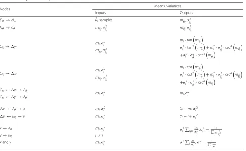
Finally, the estimated coordinate position (x,y) of the unknown radio wave emitter is determined by(mx,my). To provide more comprehensive understanding, we sum-marize all equations operating at each node of the FG in
Table 1, where the directions of the message flow is shown in the left column.
4 CRLB derivation for DOA-based geolocation
This section derives the CRLB for DOA-based geoloca-tion, taking into account the number of samples. The CRLB for DOA-based geolocation is presented in [7]; however, it does not take into account the effect of num-ber of samples. The likelihood forKi.i.d. samplesθˆk, k=
{1, 2,. . .,K}, following the Gaussian distribution, is pre-sented in [19], as
p(θˆ;θ)=
omitted again for simplicity. After several mathematical manipulations, as described in the Appendix, the closed form of the second-order derivative of log-likelihood function (LLF) is expressed as [19]
∂2
Table 1The operations required for each node in the DOA-based TS FG
The closed-form CRLB for DOA-based geolocation technique which takes into account the number of sam-ples is found to be
CRLBDOA=
trace
JT−1
θ J K
−1
, (29)
where θ = σθ2IN denotes Gaussian covariance, IN
denotes anN ×N identity matrix, andJ = ∂θ∂x denotes
Jacobian matrix given by
J= ⎡ ⎢ ⎢ ⎢ ⎢ ⎢ ⎢ ⎣
Y1−y
r21 −
X1−x
r21 Y2−y
r2
2 −
X2−x
r2 2
..
. ...
YN−y
r2N −
XN−x
rN2 ⎤ ⎥ ⎥ ⎥ ⎥ ⎥ ⎥ ⎦
(30)
with theri denotes the Euclidean distance between the
target and sensors.
5 Simulation results
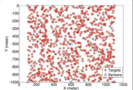
The performance of the proposed technique was verified via computer simulations, where the simulation round consists of 1000 single-target locations randomly chosen from the area of 1000×1000 m2, where each target loca-tion is tested in 100 trials. It should be noted here that the scope in this paper is to estimate only one target posi-tion. The case of unknown multiple-target detection is left for future work. It is assumed that the illegal radio, as an example of unknown radio emitter, emits the radio wave with strong enough transmit power covering the
area of 1000×1000 m2. The values of the measurement
error wereσθ = {1◦, 5◦, 10◦, 15◦,· · ·, 45◦}. It was assumed that the simulation does not contain outliers in angular measurement.
It may be difficult toachievethe LOS condition in areas
with a size of 1000 × 1000 m2 especially in (sub)urban
environments. However, instead, we can include the error due to the non-LOS components to the variance of the measurement error as shown in [20, 21], where the vari-ances are different between the sensors. For simplicity,
we assume that the variance σθ2 of the measurement
error is common to all sensors as in [6–8, 10, 11]. It is rather straightforward to derive the algorithm where each sensor has different values of variances. In fact, in our simulation setup, the area size is much smaller than that used in other references, for example, the TOA-based FG in [[8], TOA/DOA-based FG in [6], DOA-based FG in [7], and TDOA-based FG in [10], where they consider a hexagonal area with a radius of 5 km. Furthermore, as found in the simulation results, the estimation accu-racy is quite high even with relatively large variance, e.g., with standard deviationσθ =45◦. This indicates that the
assumption for the impact of the non-LOS components being represented by the measurement error variance is reasonable.
As shown in Fig. 3, six sensors were assumed in
total, indicated by the mark. The positions of the
sensors in the simulation were limited to certain
posi-tions making a sensing area with three and five
sen-sors at{(100, 0),(1100, 0),(600,−1000)}m and{(100, 0),
(1100, 0), (600,−500), (100,−1000), (1100,−1100)} m, respectively. As described above, the target positions are
randomly chosen inside the sensing 1000×1000 m2area
to evaluate the effectiveness of the proposed technique. The accuracy of the proposed technique was evaluated by using the following parameters: (a) three to five sensors taken from the total of six sensors, (b) 25 to 1000 samples, and (c) 10 times of iterations for each trial. The initializa-tion point is set at(0, 0)formx→Aθandmy→Bθand at(1, 1)
forσx2→Aθ andσy2→Bθ. It should be noted that the initial-ization point can be set arbitrarily inside the area of the expected target detection. Regardless of the target posi-tions (1000 points tested), with the initialization of mean and variance being set at(0, 0)and(1, 1), respectively, the final estimate of the target position is quite accurate. Con-versely, this observation should be understood in a way that the estimation result is less sensitive to the initial values.
To demonstrate the convergence property of the pro-posed technique, the trajectory of a detection trail is shown in Fig. 4. It shows clearly that the target position estimate successfully reaches the true target position at
(x,y)=(444,−746)m in 10 iterations, where the iteration process is started from the initial point (0,0) m. The esti-mate target position is calculated in each iteration by using (26) and (27). It should be noticed that only with seven iterations, the position estimate of the proposed technique reaches a point close to the true target position by using three sensors.
Fig. 4Trajectory of the proposed technique with 3 sensors, 10 iterations, 100 samples,σθ=10◦, and target at(444,−746)m
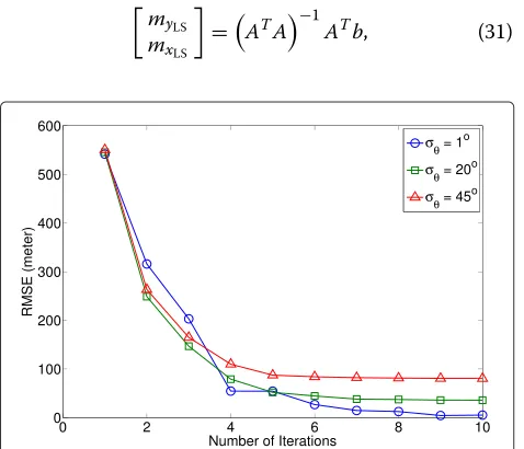
Figure 5 shows the RMSE versus the iteration times
with the standard deviationσθof the measurement error
as a parameter. The RMSE of the proposed technique converges after nine iterations forσθ = 1◦, while it con-verges after five iterations forσθ = 20◦andσθ = 45◦as shown in Fig. 5. Hence, the iteration converges faster with a higher standard deviation of the measurement error because lowerσθneeds more times to achieve better accu-racy. Although the RMSE withσθ =1◦is worse with less
than five iterations, the RMSE with smaller σθ is lower
when the iterations converges.
To make a comparison of the accuracy of the proposed technique to the conventional DOA-based LS technique in [16], we conducted another series of the conventional DOA-based LS algorithm [16] in summarized below
myLS mxLS
=ATA −1ATb, (31)
Fig. 5RMSE vs. iteration times of DOA-based TS FG geolocation technique with 3 sensors, 10 iterations, 100 samples, 1000 locations, 100 trials, andσθ= {1◦, 20◦, 45◦}
where
A =
⎡ ⎢ ⎢ ⎢ ⎢ ⎢ ⎢ ⎣
1−tan
mNθ1→Cθ1
1−tanmNθ2→Cθ2
.. . ... 1−tan
mNθN→CθN ⎤ ⎥ ⎥ ⎥ ⎥ ⎥ ⎥ ⎦
, (32)
b = ⎡ ⎢ ⎢ ⎢ ⎢ ⎢ ⎢ ⎣
Y1−X1tan
mNθ1→Cθ1
Y2−X2tan
mNθ2→Cθ2
.. .
YN−XNtan
mNθN→CθN ⎤ ⎥ ⎥ ⎥ ⎥ ⎥ ⎥ ⎦
,
with(mxLS,myLS)being the target position estimate. The
RMSEs achieved by the proposed and the conventional DOA-based LS techniques are then compared with the CRLB. In each round of simulations, both techniques used the same parameter values as described before.
Figure 6 shows that the RMSE versus the standard
devi-ation σθ of the measurement error with the number of
sensors as a parameter. It is found that the more sensors, the smaller the RMSE. Figure 7 shows the number of the sensors versus the RMSE with the standard deviationσθof the measurement error as a parameter. It is found from the figure that there is a clear difference in the tendency of the RMSE between the proposed technique and the conven-tional DOA-based LS technique. With the convenconven-tional DOA-based LS technique, the RMSE with three sensors yields better performance than that of with four sensors
forσθ = 1◦, and the RMSE with five sensors is almost
the same as that with four sensors. This indicates that since the LS equation is overdetermined with more than three sensors, the LS error is the dominant factor with
σθ = 1◦. Whenσθ = {20◦, 45◦}, on the other hand, the measurement error is the dominating factor, and hence,
Fig. 7RMSE vs. sensor number with 10 iterations, 1000 locations, 100 trials, andσθ= {1◦, 20◦, 45◦}
the achieved RMSEs with three, four, and five sensors are almost the same. This may be because the measurement error dominates the accuracy over the error due to the overdetermination.
In contrast to this observation, the RMSE decreases by increasing the sensor number forσθ = {1◦, 20◦, and 45◦} with the proposed technique, and such tendency is consis-tent to the CRLB. It can be concluded that the geolocation accuracy in terms of RMSE with the proposed technique outperforms the reference conventional DOA-based LS technique.
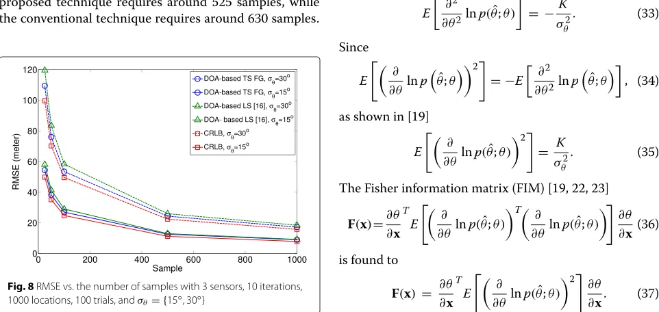
Figure 8 shows the effect of the number of samples to the accuracy of DOA-based geolocation techniques
withσθ as a parameter. The RMSE of both the proposed
and reference techniques[16] as well as the CRLB for the DOA-based geolocation decreases when more samples are used. It is shown in Fig. 8 that with RMSE 24 m, the proposed technique requires around 525 samples, while the conventional technique requires around 630 samples.
Fig. 8RMSE vs. the number of samples with 3 sensors, 10 iterations, 1000 locations, 100 trials, andσθ= {15◦, 30◦}
The accuracy of the proposed technique always outper-forms the reference technique with the same number of samples used. Obviously, by increasing the number of samples, the gap to the CRLB decreases with both the pro-posed and reference techniques. It is also found from the figure that the smaller the measurement error, the smaller
the gap to the CRLB. The gap with different σθ values
decreases when the number of samples increases.
6 Conclusions
We have proposed a new FG-based geolocation technique using DOA information for a single unknown (anony-mous) radio emitter with accuracy improvement of the position estimate. We have derived a set of new approxi-mated expression for the mean and variance of the tangent and cotangent functions based on the first-order TS to hold the Gaussianity assumption. We have also derived a closed-form expression of the CRLB for DOA-based techniques taking into account the influence of the num-ber of samples. The simulation results confirmed that our proposed technique provides (a) better accurate position estimate with the number of samples, number of sensors, and standard deviation of measurement error as parame-ters, (b) fast convergence, and (c) keep low computational complexity, which are suitable for the future geolocation techniques requiring high accuracy and low complexity in an imperfect synchronization condition. The develop-ment of DOA-based TS FG technique for multiple-target detection is left as future work.
Appendix: CRLB derivations for DOA-based geolocation
The sensor indexi is omitted in this derivation for sim-plicity. By taking the expectation of (28), we have
E ∂2
∂θ2lnp(θˆ;θ)
= −K
σ2
θ
. (33)
Since
E
∂ ∂θ lnp
ˆ θ;θ
2
= −E
∂2
∂θ2lnp
ˆ
θ;θ , (34)
as shown in [19]
E
∂
∂θ lnp(θˆ;θ) 2
= K
σ2
θ
. (35)
The Fisher information matrix (FIM) [19, 22, 23]
F(x)=∂θ ∂x
T
E
∂
∂θ lnp(θˆ;θ) T∂
∂θ lnp(θˆ;θ)
∂θ
∂x(36)
is found to
F(x) = ∂θ ∂x
T
E
∂
∂θ lnp(θˆ;θ) 2∂θ
Substituting (35) into (37) yields
F(x)= ∂θ ∂x
TK
σ2
θ
∂θ
∂x. (38)
Now, we replace θ by a vectorθ = (θ1,. . .,θN). Then, the variance(σθ2)is replaced by the Gaussian covariance matrixθ, as
F(x)=KJTθ−1J. (39)
Finally, by substituting (39) into the CRLB expression (29), as in [7, 10, 19], we obtain the CRLB for a DOA-based geolocation technique that takes into account the
measured number of samplesK, as
CRLBDOA=
trace
JT−1
θ J K
−1
.
Acknowledgements
This research is supported, in part, by Koden Electronics Co., Ltd., and in part by the Doctor Research Fellow (DRF) Program of Japan Advanced Institute of Science and Technology (JAIST).
Authors’ contributions
MRKA conceived and designed the research work, expanded and improved the algorithms for more potential applications, conducted computer simulations, acquired and analyzed data, and critically revised the manuscript. KA conceived and designed the research work, developed the base of algorithm for geolocation, analyzed data, and critically revised the manuscript. TM conceived and designed the research work, performed verification of the algorithm, analyzed data, and critically revised the manuscript. All authors read and approved the final manuscript.
Competing interests
The authors declare that they have no competing interests.
Author details
1School of Information Science, Japan Advanced Institute of Science and
Technology (JAIST), 1-1 Asahidai, Nomi-shi 923-1292, Japan.2Electrical Enginering Department, Institut Teknologi Sumatera (ITERA), Lampung Selatan 35365, Indonesia.3Centre for Wireless Communications (CWC), University of Oulu, 90014 Oulu, Finland.
Received: 25 April 2015 Accepted: 5 August 2016
References
1. J James, J Caffery, GL Stuber, Overview of radiolocation in CDMA cellular systems. IEEE Commun. Mag.36(4), 38–45 (1998)
2. K Pahlavan, X Li, J-P Makela, Indoor geolocation science and technology. IEEE Commun. Mag.40, 112–118 (2002)
3. Y Zhao, Standardization of mobile phone positioning for 3G systems. IEEE Commun. Mag.40, 108–116 (2002)
4. J-C Chen, C-S Maa, J-T Chen, inProc. IEEE International Conference on Acoustics, Speech, and Signal Processing (ICASSP) 2003. Factor graphs for mobile position location, vol. 2, (2003), pp. 393–396
5. FR Kschischang, BJ Frey, H-A Loeliger, Factor graphs and the sum-product algorithm. IEEE Trans. Inf. Theory.47(2), 498–519 (2001)
6. J-C Chen, P Ting, C-S Maa, J-T Chen, inIEEE VTC 2004. Wireless geolocation with TOA/AOA measurements using factor graph and sum-product algorithm, vol. 5, (2004), pp. 3526–3529
7. B Omidali, SA-AB Shirazi, in14th International CSI Computer Conference (CSICC 2009). Performance improvement of AOA positioning using a two-step plan based on factor graphs and the Gauss-Newton method, (2009), pp. 305–309
8. J-C Chen, Y-C Wang, C-S Maa, J-T Chen, Network side mobile position location using factor graphs. IEEE Trans. Wireless Comm.5(10), 2696–2704 (2006)
9. J-C Chen, C-S Maa, J-T Chen, Mobile position location using factor graphs. IEEE Commun. Lett.7, 431–433 (2003)
10. C Mensing, S Plass, Positioning based on factor graphs. EURASIP J. Adv. Signal Process.2007(ID 41348), 1–11 (2007)
11. C-T Huang, C-H Wu, Y-N Lee, J-T Chen, A novel indoor RSS-based position location algorithm using factor graphs. IEEE Trans. on Wireless Comm.
8(6), 3050–3058 (2009)
12. G Giorgetti, A Cidronali, SKS Gupta, G Manes, Single-anchor indoor localization using a switched-beam antenna. Commun. Letters, IEEE.
13(1), 58–60 (2009)
13. J Wang, J Chen, D Cabric, Cramer-Rao bounds for joint RSS/DOA-based primary-user localization in cognitive radio networks. IEEE Trans. Wireless Commun.12(3), 1363–1375 (2013)
14. DG Gregoire, GB Singletary, inAerospace and Electronics Conference, 1989. NAECON 1989., Proceedings of the IEEE 1989 National. Advanced ESM AOA and location techniques, (1989), pp. 917–9242
15. SZ Kang, Z Ming, inAerospace and Electronics Conference, 1988. NAECON 1988., Proceedings of the IEEE 1988 National. Passive location and tracking using DOA and TOA measurements of single nonmaneuvering observer, (1988), pp. 340–3441
16. P Kulakowski, J Vales-Alonsob, E Egea-Lopez, W Ludwin, J Garcá-Haro, Angle-of-arrival localization based on antenna arrays for wireless sensor networks. Comput. Electr. Eng.36, 1181–1186 (2010)
17. N O’Donoughue, JMF Moura, On the product of independent complex Gaussians. IEEE Trans. Signal Process.60(3), 1050–1063 (2012) 18. G Casella, RL Berger,Statistical inference, 2nd edn., (Duxbury, 2002) 19. SM Kay,Fundamentals of statistical signal processing: estimation theory.
(Prentice Hall, 1993)
20. H-L Jhi, J-C Chen, C-H Lin, A factor-graph-based TOA location estimator. IEEE Commun. Mag.11(5), 1764–1773 (2012)
21. MP Wylie, J Holtzman, The non-line of sight problem in mobile location estimation. IEEE Trans. Signal Process, 827–831 (1996)
22. C Gentile, N Alsindi, R Raulefs, C Teolis,Geolocation techniques, principles and applications. (Springer, New York, 2013)
23. G Mao, B Fidan,Localization algorithms and strategies for wireless sensor networks: monitoring and surveillance techniques for target tracking. (IGI Global, New York, 2009)
Submit your manuscript to a
journal and benefi t from:
7 Convenient online submission
7 Rigorous peer review
7 Immediate publication on acceptance
7 Open access: articles freely available online
7 High visibility within the fi eld
7 Retaining the copyright to your article