Earth Planets Space,61, 237–247, 2009
Analyzing the variation of embedding dimension of solar and geomagnetic
activity indices during geomagnetic storm time
M. Mirmomeni1and C. Lucas1,2
1Control and Intelligent Processing Center of Excellence, College of Engineering, School of Electrical and Computer Engineering, University of Tehran, Tehran, Iran
2School of Cognitive Sciences, Institute for studies in theoretical Physics and Mathematics, Tehran, Iran
(Received March 21, 2008; Revised August 3, 2008; Accepted September 7, 2008; Online published February 18, 2009)
Cyclic solar activity as one of the natural chaotic phenomena has significant effects on Earth, climate, and satellites. Rapid changes in the near-Earth space environment can affect the performance and reliability of both spacecraft and ground-based systems. This can imply major problems due to communication and satellite operational anomalies. Therefore, it is meaningful to analyze solar activity and geomagnetic indices to elicit the behavior of sun as the origin of most of these chaotic phenomena. One of the most important tools for analyzing the chaotic trends is the “Embedding Dimension” (ED). In this paper, the variation of ED for solar activity indices especially during storm time for two well-known storms is considered. The first storm is the super-storm on 13 March 1989, which shuts down the power supply system in Qu´ebec, Canada and the second one is the storm caused by Coronal Mass Ejection on 11 January 1997 which causes the failure of Telstar 401 satellite. The method of this paper is based on the fact that the reconstructed dynamics of an attractor should be a smooth map, i.e. with no self intersection in the reconstructed attractor. It is shown that the Embedding Dimension (and other chaotic characteristics) of some solar and geomagnetic activity indices during these storms varies rapidly.
Key words: Space weather, chaotic dynamics, embedding dimension, polynomial models, solar activity, geo-magnetic activity, geogeo-magnetic storms.
1.
Introduction
Recently, there has been so much progress made in so-lar plasma eruptions, geomagnetic storms and sub-storms that the time is now ripe to put all related and global as-pects together into a field of space weather. On the other hand, technological progress was made in 20th century and continued in the beginning of 21st century has made hu-man life increasingly dependent on satellites. There has been a rapidly increasing reliance on spacecraft systems to meet modern human needs for information transfer and re-mote sensing (Baker, 2000). As human presence in space is in an explosive phase, it is expected that the impact of these effects will be quite significant in this and the next solar cycles (Vassilidiadis, 2000; Sharifiet al., 2006; Mir-momeniet al., 2006, 2007). In addition, modern satellite systems and subsystems appear to show an increasing sus-ceptibility to effects of the space weather due to their high-sensitive electronic nature (Baker, 2000). Space weather not only affects the functioning of technical systems in space and on Earth, but may also endanger human health and life (Hill et al., 2000; Carlowicz and Lopez, 2002). The ef-fects of this phenomenon are many and varied: they include electronic failures (Loveet al., 2000; Dorman, 2005), im-mediate and long term hazards to astronauts and aircraft crews (Garrett and Hoffman, 2000; Jokiaho, 2004; Defise
Copyright cThe Society of Geomagnetism and Earth, Planetary and Space Sci-ences (SGEPSS); The Seismological Society of Japan; The Volcanological Society of Japan; The Geodetic Society of Japan; The Japanese Society for Planetary Sci-ences; TERRAPUB.
et al., 2005), changes in electrostatic charging of satellites (Lai, 1996, 1999; Baker, 2000), interruptions in telecom-munications and navigational systems (Boteleret al., 1998; Kikuchi, 2003; Stanislawskaet al., 2003), and power trans-mission failures (Kappenman, 1999; Pirjola, 1998; Daglis et al., 2004) and disruption to rail traffic signaling (Label and Barth, 2000; Pirjola, 2003). Space weather is thus a lot more than the impressive auroras at high latitudes, with which we are all familiar and risk hazards due to space weather exotic phenomena pose serious threat motivating rapid search for accurate analyzing, modeling, and predic-tion methods (Turner, 2000; Bothmer, 2004).
It is shown that the cyclic solar activity has chaotic char-acteristics especially during storm time which depicts the difficulties in long-term prediction of solar activity indices (Stefanski, 2003; Gholipouret al., 2007; Mirmomeniet al., 2007). It has to be said that, deterministic chaos appears in different fields of science like physics, biomedicine, and engineering (Ruelle, 1978; Kocarevet al., 2006). The main idea of chaotic time series analysis is that a complex system can be described by a strange attractor in the phase space (Mirmomeni and Lucas, 2008). The first step of chaotic time series analysis is the reconstruction of the equivalent attractor’s state space. State space reconstruction can be de-scribed by embedding the time series in a vector space. The embedding theorem is proposed by Takens (Takens, 1981; Saueret al., 1991). However, Takens’ theorem is valid for indefinite noise free data only and does not address the cal-culation of embedding dimension and lag time. In addition,
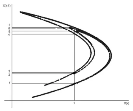
Fig. 1. Strange attractor of a two dimensional chaotic system, if order is under-estimated tod = 1 all the points 1, . . . ,7 onx(k−1)axis are projected on point 1 inx(k)axis and have the same one step ahead value.
it is of little practical relevance since it suggests a sufficient condition based on the dimension of the attractor’s mani-fold, which is not known a priori. There are many publica-tions concerning the estimation of suitable embedding di-mension from chaotic time series. They can be summarized in three main categories as follow.
The first approach is based on the fact that the original at-tractor lies on a smooth manifold. This condition is checked by different methods by many researchers. The most fa-mous work seems to be the method of False Nearest Neigh-bours (FNN) developed in Kennelet al.(1992). The second approach for estimating the embedding dimension is based on Singular Value Decomposition (SVD) method which is proposed in Broomhead and King (1986) and Cao (1997). The main idea of this approach is to obtain a base for the embedding space in such a way that the attractor can be modelled by an invariant geometry in a subspace with fixed dimension. It has to be said that, many researchers doubt in the quality of this method in eliciting the characteristics of nonlinear time series because the SVD essentially is a linear approach with firm theoretic base (Messet al., 1987; Fraser, 1989; Bian and Ning, 2004; Menget al., 2007). The third approach is based on considering an invariant on the attrac-tor such as correlation dimension (Grassberger and Procac-cia, 1983), successive values of embedding dimension and convergent values. The typical problems of this method are its computation time, its poor performance for short time series, and its sensitivity to noise (Menget al., 2007).
In this paper, it is tried to elicit the variation of chaotic trends of solar activity indices, especially during storm time. Eliciting the variation of chaotic trends is the first step for modeling such complex and chaotic phenomena. To achieve this, there are some quantitative measures including fractal dimension, entropy and Lyapunov exponents (LEs) (Sano and Sawada, 1985; Chenet al., 2006; Liuet al., 2005; Serletiset al., 2007).
In this paper, the variation of embedding dimension from some solar activity indices based on polynomial models is considered. This method has been used in many
applica-tions by several researchers (e.g., Ataeiet al., 2003, 2004; Bian and Ning, 2004; Meng et al., 2007) and the perfor-mance of this method in estimating the optimal embedding dimension even for noisy chaotic dynamics is great (Meng et al., 2007). In addition, this method is applicable to short time series as well and its performance for estimating em-bedding dimension of noisy chaotic dynamic is good (Bian and Ning, 2004; Menget al., 2007). In this method a gen-eral polynomial autoregressive model (Landauet al., 1989; Isermann, 1991; Ljung, 1998; Nelles, 2001), is considered to locally fit the given data. The order of this model is the same as the dimension of the reconstructed state space. The reconstructed dynamics should be a smooth map, i.e. with no self-intersection in the reconstructed attractor. This property is checked by the evaluation of the one step ahead prediction error of the fitted model for different orders and various degrees of nonlinearity in the polynomials. The minimum embedding dimension is determined as the or-der with which the level of the prediction error decreases abruptly. It is shown that this approach has the capability of adaptively computing embedding dimension of uncer-tain or time varying chaotic dynamical systems (Ataeiet al., 2004). Therefore, it is useful to apply this adaptive estima-tion method to elicit the variaestima-tion of ED for solar activity indices. To show the variation of ED of solar activity in-dices, two well-known storms are considered. The first one is the super-storm on 13 March 1989 which cause a black out about nine hours in Qu´ebec, Canada and the second one is the storm caused by Coronal Mass Ejection (CME) on 11 January 1997 which causes the most widely known dis-turbances and failures for satellites: the failure of Telstar 401 satellite. In this paper, ED of three solar activity and some other related indices is estimated via proposed adap-tive approach: Sunspot number, Disturbance Storm Time (Dst) and Proton temperature as one of the factors of solar
wind index. The results of this paper depict that the embed-ding dimension (and chaotic characteristics) of these solar activity indices during these storms vary rapidly.
The remaining sections of this paper are structured as follows: the main idea of the method for estimating the minimum embedding dimension is presented in Section 2. Model based procedure for estimation of the embedding di-mension is presented in Section 3. Section 4 is devoted to describe the performance of the proposed method in elic-iting the variation of chaotic characteristics of solar activ-ity indices especially during storm time by estimating min-imum embedding dimension of solar activity indices. The last section contains the concluding remarks.
2.
Model Based Estimation of the Embedding
Di-mension
In this section, the basic idea and the procedure of the model based method for estimating the embedding dimen-sion is presented. Let the original attractor of the system exists in anm-dimensional smooth manifold, M. The dy-namical behavior of the system is not known a priori and only a sequence of measurements is available as follows,
y(t+ts),y(t+2ts), . . . ,y(t+N ts)≡y1,y2, . . . ,yN
M. MIRMOMENI AND C. LUCAS: ANALYZING THE VARIATION OF EMBEDDING DIMENSION 239
Fig. 2. Daily average ofDstindex during 1989.
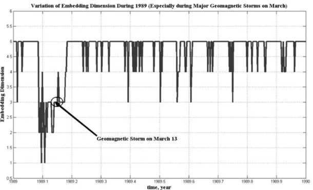
Fig. 3. Variation of the minimum embedding dimension ofDstindex during 1989.
wheretsis the sampling time and N is the total number of
measurements.
An embedding is a smooth map from the manifold M to spaceU in such a way that its image be a smooth sub-manifold ofU. It has to be said that this map is a diffeomor-phism betweenM and its image. By using Method of De-lays (Takens, 1981; Mirmomeni and Lucas, 2008), which is based on Takens’ theorem, the embedding space is recon-structed by d (greater than 2m) sequential values of mea-surements as:
[y((k−(d−1))ts) ,y((k−(d−2))ts) , . . . ,
y((k−1)ts) ,y(kts)] (2)
where ts is the sampling time and the dimension of the
reconstructed space, d is called the embedding dimension (its optimal value is looked for).
The attractor of the well reconstructed phase space is equivalent to the original attractor and should be expressed as a smooth map. The state equations of the reconstructed
dynamics are considered as:
x(k+1)= f x(k) (3) where f(.)is a continuously differentiable function to the state vectorx(k). In many practical situations, the structure of the underlying dynamical system is unknown. Depend-ing on the objectives, there are different theories which are suitable for special analysis of nonlinear systems. In this paper, in order to model the reconstructed state space, the vector (2) after normalization, is considered as the state vec-tors.
x(k)=
⎡ ⎢ ⎢ ⎢ ⎣
x1(k)
x2(k)
...
xd(k)
⎤ ⎥ ⎥ ⎥
⎦=
⎡ ⎢ ⎢ ⎢ ⎣
y(k−(d−1)) y(k−(d−2))
...
y(k)
⎤ ⎥ ⎥ ⎥
⎦ (4)
Fig. 4. Variation of one step ahead prediction error calculated for the estimated embedding dimension and degree of nonlinearity of the polynomial models ofDstindex during storm on March 1989.
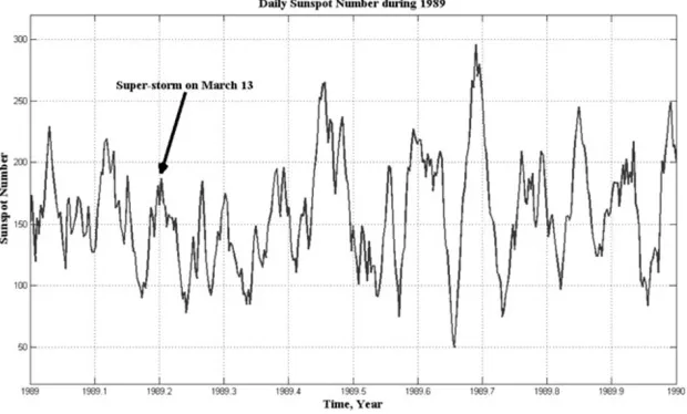
Fig. 5. Daily average SSN index during 1989.
by polynomial modeling as follows:
y(k+1)=gx(k) (5) A canonical state space representation of the system is obtained as follows:
x(k+1)=
⎡ ⎢ ⎢ ⎢ ⎣
y(k−d+2) y(k−d+3)
...
y(k+1)
⎤ ⎥ ⎥ ⎥
⎦=
⎡ ⎢ ⎢ ⎢ ⎣
x2(k)
x3(k)
...
gx(k)
⎤ ⎥ ⎥ ⎥
⎦ (6)
Thus, the order of polynomial model g(.) will also be d. Therefore, the optimal embedding dimension and the suitable order of the polynomial model have the same value. Now, let us have an example to show the main idea of finding the optimal embedding dimension for a chaotic dy-namic. Consider for example a two dimensional nonlinear chaotic system with its strange attractor as shown in Fig. 1. The phase diagram or state trajectory which is shown in
Fig. 1 depicts the chaotic trends of this dynamic. The objec-tive is to find a model as Eq. (5) by using the autoregressive polynomial structure. If the order of the model is under-estimated tod =1, it is obvious from Fig. 1 that the model will project seven points(i,1),i =1, . . . ,7 to the same one step ahead value, sayxˆk+1. Therefore, the first step ahead
prediction error for each transition of the point is:
e(i,1)= ˆxk+1−xk+1(i,1) (7)
i =1, . . . ,7 (Number of points proejcted to the same
one step ahead value)
wherexk+1(i,1)denotes the true first step ahead value. By
this assumption for embedding dimension, these errors will be large since only one fixed projection has been considered for all of these points. If the order of model is selected to d = 2, then for each points of xk+1(i,1), i = 1, . . . ,7
M. MIRMOMENI AND C. LUCAS: ANALYZING THE VARIATION OF EMBEDDING DIMENSION 241
Fig. 6. Variation of the minimum embedding dimension of SSN index during 1988 and 1989.
Fig. 7. Variation of one step ahead prediction error calculated for the estimated.
error in this case is:
e(i,1)= ˆxk+1(i,1)−xk+1(i,1) (8)
i =1, . . . ,7 (Number of points proejcted to the same
one step ahead value)
The errors in this case are much smaller than the previous case, since the error in this analysis shows only the capabil-ity of selected model in predicting one step ahead value of chaotic dynamic. In addition, the mean squares of these er-rors for all points of the strange attractor differ so much in these two different choices. Typically, it is observed that the mean squares of prediction errors decrease whiled in-creases; however if one continues to increase the value of d, there will be a value ford (or an order for state space of the model) which the change ond has no effects on predic-tion error. This order is the best choice for the order of the model and is selected as minimum embedding dimension as well.
In the following section, by using the aforementioned idea, the procedure of estimating the minimum embedding dimension for chaotic time series is presented.
3.
Model Based Procedure for Estimation of the
Embedding Dimension
The procedure for estimation of the embedding dimen-sion of chaotic time series consists of 7 steps as follows:
Fig. 8. DailyDstindex during 1997.
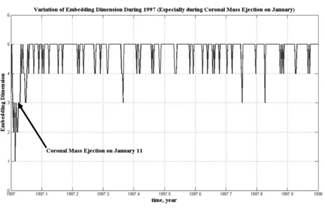
Fig. 9. Variation of the minimum embedding dimension ofDstindex during 1997.
2) Some definite ranges for embedding dimension and degree of nonlinearity of the polynomial models have to be chosen such as
D= {1,2, . . . ,dmax}
Np= {1,2, . . . ,nmax}
(9)
3) For eachdi∈ Dconstruct the delayed vector as
x(k)=
⎡ ⎢ ⎢ ⎢ ⎣
y(k−(di−1))
y(k−(di−2))
...
y(k)
⎤ ⎥ ⎥ ⎥
⎦ (10)
4) For each delayed vector (10), findr nearest neighbors whichr as a designing parameter should be greater thanmas defined by Ataeiet al.(2003, 2004):
m= (di+ni)! di!ni!
(11)
where di and n are the model order and degree of
nonlinearity respectively.
5) The following polynomial autoregressive model (Iser-mann, 1991; Ljung, 1998) is fitted to the set of neigh-bors found in the last step by well-known Least Square (LS) technique (Isermann, 1991; Ljung, 1998; Nelles, 2001).
y(k+1)=θ0+ di−1
i=0
θ1iy(k−i)
+ di−1
i=0 di−1
j=i
θ2i jy(k−i)y(k− j)
+ di−1
i=0 di−1
j=i di−1
p=j
θ3i j py(k−i)y(k−j)y(k−p)+ · · ·
+ di−1
i=0 di−1
j=i · · ·
di−1
v=u
θnii j p···uvy(k−i)y(k− j)· · ·
M. MIRMOMENI AND C. LUCAS: ANALYZING THE VARIATION OF EMBEDDING DIMENSION 243
Fig. 10. Variation of one step ahead prediction error calculated for the estimated embedding dimension and degree of nonlinearity of the polynomial models ofDstindex during CME on January 1997.
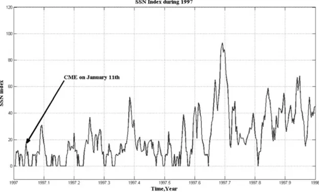
Fig. 11. Daily SSN index during 1997.
The initial values of parameters in vector which should be tuned by least square technique are chosen randomly. For the model orderdi and degree of
non-linearityn the number of parameters in vectorthat should be estimated to identify the underlying model can be calculated via Eq. (11).
6) The mean square of prediction errors is computed as:
σ =
1
N
N
k=1
e2k=
1
N
N
k=1
ˆ
x(k)−x(k)2 (13)
whereNis the total number of points andekis the one
step ahead prediction error.
7) The one step ahead prediction error should be calcu-lated for all embedding dimension and degree of non-linearity of the polynomial models by above procedure (the full range of DandNp). By plotting the level of
prediction error vs. model order, the minimum embed-ding dimension can be considered as the model order
d∗which the variation of prediction error is negligible ford >d∗.
As it said before, this method has the following advan-tages, it is (1) applicable to a short time series, (2) stable to noise, (3) computationally efficient (typically, the anal-ysis of a 500-point time series takes just a few seconds on a desktop computer), and (4) without any purposely intro-duced parameters (Bian and Ning, 2004; Menget al., 2007).
4.
Case Studies
This section is devoted to elicit the variation of embed-ding dimension of some solar activity and other related in-dices such as sunspot number (SSN), Disturbance storm time (Dst) as an important measure for predicting magnetic
storms and Proton temperature as an important factor of so-lar wind index during storm time. Two well-known storms are considered in this section.
interplan-Fig. 12. Variation of the minimum embedding dimension of SSN index during 1997.
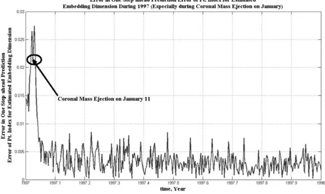
Fig. 13. Variation of one step ahead prediction error calculated for the estimated embedding dimension and degree of nonlinearity of the polynomial models of SSN index during CME on January 1997.
etary magnetic field (IMF) and solar wind plasma parame-ters measured by various spacecrafts near the Earth’s orbit, as well as geomagnetic and solar activity indices, and ener-getic proton fluxes. This data set was created at NSSDC in 2003 as a successor to the OMNI data set first created in the mid-1970’s. A detailed discussion of the creation OMNI 2 is at http://nssdc.gsfc.nasa.gov/omniweb/.
4.1 Case study 1: variation of ED during magnetic storm on 13 March 1989
This subsection is devoted to elicit the variation of ED of two important solar and geomagnetic activity indices during super-storm on 13 March 1989. It has to be said that the proton temperature of solar wind index was not saved during this storm. Therefore in this subsection the variation of ED for SSN andDstindices are analyzed.
The proposed method for estimating the embedding di-mension or suitable order of model based on local poly-nomial modeling is implemented to these solar activity in-dices as some chaotic time series. For these time series,
the developed general program of polynomial modeling is applied for variousd andn, andσ is computed for all the cases in a look up table. After that, based on the discussions in Sections 2 and 3, the optimum embedding dimension is selected for these time series in each step.
M. MIRMOMENI AND C. LUCAS: ANALYZING THE VARIATION OF EMBEDDING DIMENSION 245
Fig. 14. Daily proton temperature index during 1997.
Fig. 15. Variation of the minimum embedding dimension of proton temperature index during 1997.
average of Dst index during 1989. The drop off during
March depicts the major magnetic storm which caused the black out in Quebec.
It has to be said that, the estimated embedding dimen-sion for overallDstindex is equal to 5. Figure 3 shows the
variation of the minimum embedding dimension of Dst
in-dex during 1988 and 1989. The variation of ED is large and there is an obvious oscillation before storm onset. Fig-ure 4 shows the variation of the one step ahead prediction error calculated for the estimated embedding dimension and degree of nonlinearity of the polynomial models by above procedure during storm on March 1989. It is obvious that the one step ahead prediction error increases rapidly before storm and during the storm time which shows the varia-tion of chaotic characteristics of this natural chaotic phe-nomenon.
Again, for SSN, the developed general program of poly-nomial modeling is applied to estimate the minimum em-bedding dimension of this chaotic dynamic. Figure 5 shows the hourly SSN during 1989. During this magnetic
super-storm, the SSN is high.
Figure 6 shows the variation of the ED of SSN during 1988 and 1989. It is obvious that the variation of ED is not as large as the variation of ED of Dst Index; however
there is a rapid oscillation right before storm beginning for this index too. Figure 7 shows the variation of the one step ahead prediction error for estimated embedding dimension of SSN during March 1989. It is obvious that the one step ahead error increases rapidly during this storm.
4.2 Case study 2: variation of ED during CME on 11 January 1997
This subsection is devoted to elicit the variation of ED of three important solar and geomagnetic activity indices during a Coronal Mass Ejection on 11 January 1997 which was a result of events with signs started even at 6 January 1997.
Fig. 16. Variation of one step ahead prediction error calculated for the estimated embedding dimension and degree of nonlinearity of the polynomial models of proton temperature index during CME on January 1997.
off during January depicts the CME.
Figure 9 shows the variation of the ED ofDstindex
dur-ing 1996 and 1997. It can be seen that the variation of ED is not as large as the variation of embedding dimension on March 13th and there is not an oscillation before storm on-set because this hazard happened by a CME as a singular phenomenon. Figure 10 shows the variation of the one step ahead prediction error calculated for the estimated embed-ding dimension and degree of nonlinearity of the polyno-mial models by above procedure during CME on January 1997. It is obvious that the one step ahead prediction error increases rapidly before CME and during the CME.
Again, for SSN, the proposed adaptive estimation al-gorithm is applied for estimation of minimum embedding dimension of this chaotic dynamic. Figure 11 shows the hourly SSN during 1997.
Figure 12 shows the variation of the ED of SSN during 1996 and 1997. It is obvious the ED varies rapidly during this storm. Therefore, it is meaningful to use the variation of the minimum embedding dimension to alarm space weather hazards. Figure 13 shows the variation of the one step ahead prediction error for estimated embedding dimension of SSN during CME on January 1997. It is obvious that the one step ahead error increases rapidly during this CME.
Like Dstand SSN indices, for proton temperature factor
of solar wind index which is an important measure during a solar storm, the proposed estimation method is applied to estimate minimum embedding dimension. Figure 14 shows the hourly proton temperature index during 1997. The large temperature during January depicts the CME.
Figure 15 shows the variation of the ED of proton tem-perature index during 1996 and 1997. It can be seen that the variation of ED is large and there is an obvious pattern before storm beginning and variation of embedding dimen-sion clearly shows the impact of this CME. Figure 16 shows the variation of the one step ahead prediction error for es-timated embedding dimension of proton temperature index during CME on January 1997. It is obvious that the one step ahead error increases rapidly during this CME.
5.
Discussion and Conclusions
In this paper, it is tried to elicit the variation of chaotic trends of solar activity indices such as sunspot number,Dst
and proton temperature during storm time by estimating the minimum embedding dimension via an improved estima-tion method based on polynomial modelling. Two well-known storms are considered in this paper. The first one is the magnetic super-storm which caused the nine hours black out in Quebec, Canada on 13 March 1989 and the sec-ond one is a storm caused by Coronal Mass Ejection on 11 January 1997 which caused the most well-known satellite failure. The results of analysis on estimation and variation of embedding dimension depict that there is a rapid change with an obvious oscillation of ED of these solar activity in-dices during these storms. The ED of these solar activity indices begins to vary in such a way that an obvious pattern can be detected about 10 steps sooner before storm begins. Considering this fact that the hazard on 11 January was hap-pened by a CME as a singular phenomenon, the oscillation in estimated embedding dimension can not been detected easily. However, this hazard can be detected by looking to the one step ahead prediction error of embedding dimen-sion. Therefore, it is meaningful to use the variation of ED for alarming systems against space weather hazards.
Acknowledgments. The authors wish to thank the “National Space Science Data Center” for using this data set.
References
Ataei, M., A. Khaki-Sedigh, B. Lohmann, and C. Lucas, Model based method for determining the minimum embedding dimension from chaotic time series univarite and multivariate cases,Nonlinear Phenom. Compl. Syst.,6(4), 842–851, 2003.
Ataei, M., A. Khaki-Sedigh, B. Lohmann, and C. Lucas, Model based method for estimating an attractor dimension from uni/multivariate chaotic time series with application to Bremen climatic dynamics, Chaos,Solitons Fractals,19, 1131–1139, 2004.
Baker, D. N., The occurrence of operational anomalies in spacecraft and their relationship to space weather,IEEE Trans. Plasma Sci.,28(6), 2007–2016, 2000.
M. MIRMOMENI AND C. LUCAS: ANALYZING THE VARIATION OF EMBEDDING DIMENSION 247
13(5), 633–936, 2004.
Boteler, D. H., R. Pirjola, and H. Nevanlinna, The effects of geomagnetic disturbances on electrical systems at the earth’s surface,Adv. Space Res. J.,22(1), 17–27, 1998.
Bothmer, V., The solar and interplanetary causes of space storms in solar cycle 23,IEEE Trans. Plasma Sci.,32(4), 1411–1414, 2004.
Broomhead, D. S. and G. P. King, Extracting qualitative dynamics from experimental data,Phys. D,20, 217–236, 1986.
Cao, L., Practical method for determining the minimum embedding di-mension of a scalar time series,Phys. D,110, 43–50, 1997.
Carlowicz, M. J. and R. E. Lopez,Storms from the Sun: The Emerging Science of Space Weather, Joseph Henry Press, 2002.
Chen, Z. M., K. Djidjeli, and W. G. Price, Computing Lyapunov exponents based on the solution expression of the variational system,Appl. Math. Comput.,174, 982–996, 2006.
Daglis, I. A., D. Delcourt, F. A. Metallinou, and Y. Kamide, Particle accel-eration in the frame of the storm-substorm relation,IEEE Trans. Plasma Sci.,32(4–1), 1449–1454, 2004.
Defise, J. M.et al., SWAP and LYRA: space weather from a small space-craft,2nd Int. Conf. on Recent Advances on Space Technologies 2005 (RAST2005), 9–11th June, 2005.
Dorman, L. I., Forecasting of great radiation hazard: estimation of particle acceleration and propagation parameters by possible measurements of gamma rays generated in interactions of sep with upper corona and solar wind matter,2nd Online Proceeding on European Space Weather Week, ESA-ESTEC, Noordvijk, Netherland, 14–18th November, 2005. Fraser, M., Reconstructing attractors from scalar time series: A comparison
of singular system and redundancy criteria,Phys. D,34, 391–404, 1989. Garrett, H. B. and A. R. Hoffman, Comparison of spacecraft charging environments at the Earth, Jupiter, and Saturn,IEEE Trans. Plasma Sci., 28(6), 2048–2057, 2000.
Gholipour, A., C. Lucas, B. N. Araabi, M. Mirmomeni, and M. Shafiee, Extracting the main patterns of natural time series for long-term neuro-fuzzy prediction,J. Neural Comput. Appl.,16(4–5), 383–393, 2007. Grassberger, P. and I. Procaccia, Measuring the strangeness of strange
atractors,Phys. D,9, 189–208, 1983.
Hill, F., W. Erdwurm, D. Branston, and R. McGraw, The National Solar Observatory Digital Library—a resource for space weather studies,J. Atmos. Sol.-Terr. Phys.,62, 1257–1264, 2000.
Isermann, R., Adaptive control systems, Prentice-Hall, Inc., Englewood Cliffs, New Jersey, 1991.
Jokiaho, O. P., Impact of space weather on satellite operations and ter-restrial systems,55th Int. Astronautical Congress of the International Astronautical Federation, the International Academy of Astronautics, and the International Institute of Space Law, Vancouver, Canada, 4–8th October, 2004.
Kappenman, J. G., Geomagnetic storm and power system impacts: ad-vanced storm forecasting for transmission system operations,Power En-gineering Society Summer Meeting, 18–22th July, 1999.
Kennel, M. B., R. Brown, and H. D. I. Abarbanel, Determining embedding dimension for phase space reconstruction using a geometrical construc-tion,Phys. Rev. A,45, 3403–3411, 1992.
Kikuchi, T., Space weather hazards to communication satellites and the space weather forecast system,21st Int. Communications Satellite Sys-tems Conference and Exhibit, Yokohama, Japan, 15–19th April, 2003. Kocarev, K., J. Szczepanski, J. M. Amig´o, and I. Tomovski, Discrete
chaos-I: Theory,IEEE Trans. Circuit Syst.-I,53(6), 1300–1309, 2006. Label, K. A. and J. L. Barth, Radiation effects on emerging technologies—
implications of space weather risk management,AIAA Space 2000 Con-ference and Exposition, Long Beach, CA, 19–21th September, 2000. Lai, S. T., What measurements in space weather are needed for predicting
spacecraft charging?,IEEE Int. Conf. Plasma Sci., 3–5th June, 1996. Lai, S. T., DSCS satellite dielectric charging correlation with magnetic
activity,IEEE Int. Conf. Plasma Sci. (ICOPS’99), 20–24th June, 1999.
Landau, I. D., R. Lozano, and M. M’Saad,Adapted Control, Speringer-Verlag, 1989.
Liu, H. F., Z. H. Dai, W. F. Li, X. Gong, and Z. H. Yu, Noise robust estimates of the largest Lyapunov exponent,Phys. Lett. A,341, 119– 127, 2005.
Ljung, L.,System identification: theory for the user, Prentice-Hall, Inc., Englewood Cliffs, New Jersey, 1998.
Love, D. P., D. S. Toomb, D. C. Wilkinson, and J. B. Parkinson, Penetrating electron fluctuations associated with GEO spacecraft anomalies,IEEE Trans. Plasma Sci.,28(6), 2075–2084, 2000.
Meng, Q.-F., Y.-H. Peng, and P.-J. Xue, A new method of determining the optimal embedding dimension based on nonlinear prediction,Chin. Phys.,16(5), 1252–1257, 2007.
Mess, A. I., P. E. Rapp, and L. S. Jennings, Singular-value decomposition and embedding dimension,Phys. Rev. A,36, 340–346, 1987.
Mirmomeni, M. and Lucas C., Model based method for determining the minimum embedding dimension from solar activity chaotic time series,
Int. J. Eng., Trans. A: Basics,21(1), 31–44, 2008.
Mirmomeni, M., M. Shafiee, C. Lucas, and B. N. Araabi, Introducing a new learning method for fuzzy descriptor systems with the aid of spectral analysis to forecast solar activity,J. Atmos. Sol.-Terr. Phys.,68, 2061–2074, 2006.
Mirmomeni, M., C. Lucas, B. N. Araabi, and M. Shafiee, Forecast-ing sunspot numbers with the aid of fuzzy descriptor models,Space Weather,J. Res. Appl., doi:10.1029/2006SW000289, 2007.
Nelles, O.,Nonlinear system identification, Springer Verlag, Berlin, 2001. Pirjola, R., Space weather and risk management,54th Int. Astronautical Congress of the International Astronautical Federation, the Interna-tional Academy of Astronautics, and the InternaInterna-tional Institute of Space Law, Bremen, 29–3rd September, 2003.
Pirjola, R., A. Viljanen, O. Amm, and A. Pulkkinen, 1999: Power and pipelines (ground systems),the Proceeding of the ESA Workshop on Space Weather, ESTEC, Noordwijk, Netherlands, 11–13th November, 1998.
Ruelle, D., Dynamical system with turbulence behaviour,Lecture Notes in Physics,80, 341–360, 1978.
Sano, M. and Y. Sawada, Measurement of the Lyapunov spectrum from a chaotic time series,Phys. Rev. Lett.,55(10), 1082–1085, 1985. Sauer, T., J. A. Yorke, and M. Casdagli, Embedology, J. Stat. Phys.,
65(3/4), 579–616, 1991.
Serletis, A., A. Shahmoradi, and D. Serletis, Effect of noise on estimation of Lyapunov exponents from a time series, Chaos,Solitons Fractals,32, 883–887, 2007.
Sharifi, J., B. N. Araabi, and C. Lucas, Multi-step prediction of Dst. index using singular spectrum analysis and locally linear neurofuzzy model-ing,Earth Planets Space,58(3), 331–341, 2006.
Stanislawska, I., P. Bradley, Z. Klos, and H. Rothkaehl, Physical phenom-ena in ionospheric and trans-ionospheric radio-communication,the Int. Conf. on Recent Advances on Space Technologies 2003 (RAST’03), 20– 22th November, 2003.
Stefanski, A., Estimation of the largest Lyapunov exponent in systems with impacts, Chaos,Solitons Fractals,11, 2443–2451, 2003.
Takens, F., Detecting strange attractors in turbulence, inLecture Notes in Mathematics, edited by D. A. Rand and L. S. Young, Springer, Berlin, 898, 366–381, 1981.
Turner, R., Solar particle events from a risk management perspective,IEEE Trans. Plasma Sci.,28(6), 2103–2113, 2000.
Vassilidiadis, D., System identification, modeling, and prediction for space weather environments,IEEE Trans. Plasma Sci.,28(6), 1944–1955, 2000.