Basins of attraction of certain rational anti competitive system of difference equations in the plane

(1)

R E S E A R C H

Open Access

Basins of attraction of certain rational

anti-competitive system of difference

equations in the plane

Samra Moranjki´c and Zehra Nurkanovi´c

*

*_{Correspondence:} [email protected] Department of Mathematics, University of Tuzla, Tuzla, Bosnia and Herzegovina

Abstract

We investigate the global asymptotic behavior of solutions of the following anti-competitive system of rational diﬀerence equations:

xn+1=

γ

1yn

A1+xn

, yn+1=

β

2xn

A2+B2xn+yn

, n= 0, 1,. . .,

where the parameters

γ

1,

β

2,A1,A2andB2are positive numbers and the initial conditions (x0,y0) are arbitrary nonnegative numbers. We ﬁnd the basins of attraction of all attractors of this system, which are the equilibrium points and period-two solutions.

MSC: 39A10; 39A11

Keywords: diﬀerence equations; anti-competitive; map; stability; stable manifold

1 Introduction

A ﬁrst-order system of diﬀerence equations

xn+=f(xn,yn), yn+=g(xn,yn),

n= , , . . . , (x,y)∈R, ()

whereR⊂R_{, (f}_,_{g) :}_R_→_R_,_f_,_g _{are continuous functions is}_competitive_if _f_(x,_{y) is}

non-decreasing inxand non-increasing iny, andg(x,y) is non-increasing inxand non-decreasing iny.

System () where the functions f andg have a monotonic character opposite of the monotonic character in competitive system will be calledanti-competitive.

We consider the following anti-competitive system of diﬀerence equations:

xn+=

γyn A+xn

, yn+=

βxn A+Bxn+yn

, n= , , . . . , ()

where the parametersA,γ,A,Bandβare positive numbers and the initial conditions

(x,y) are arbitrary nonnegative numbers. In the classiﬁcation of all linear fractional

sys-tems in [], System () was mentioned as System (, ).

(2)

Competitive and cooperative systems of the form () were studied by many authors such as Clark and Kulenović [], Clark, Kulenović and Selgrade [], Hirsch and Smith [], Ku-lenović and Ladas [], KuKu-lenović and Merino [], KuKu-lenović and Nurkanović [, ], Garić-Demirović, Kulenović and Nurkanović [, ], Smith [, ] and others.

The study of anti-competitive systems started in [] and has advanced since then (see [, ]). The principal tool of the study of anti-competitive systems is the fact that the second iterate of the map associated with an anti-competitive system is a competitive map, and so the elaborate theory for such maps developed recently in [, , ] can be applied.

The main result on the global behavior of System () is the following theorem.

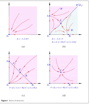
Theorem 

(a) Ifβγ≤AA, then E= (, )is a unique equilibrium, and the basin of attraction of

this equilibrium isB(E) ={(x,y) :x≥,y≥}(see Figure (a)).

(b) Ifβγ–AA> –B[A +γ(A–AB)]andβγ–AA> , then there exist two

equilibrium points: E which is a repeller and E+which is an interior saddle point, and

minimal period-two solutions A= (,βγ_γ_–_BA_A)and B= (βγ_A_–_BA_A, )which are locally

asymptotically stable. There exists a setC⊂R=[,∞)×[,∞)such that E∈C, and

Ws_(E

+) =CEis an invariant subset of the basin of attraction of E+. The setCis a graph

of a strictly increasing continuous function of the ﬁrst variable on an interval and separates

Rinto two connected and invariant components, namely

W–:=

x∈R\C:∃x ∈Cwithxsex

, W+:=

x∈R\C:∃x ∈Cwithx sex

,

which satisfy (see Figure (b)): (i) If(x,y)∈W+, then

lim

n→∞(xn,yn) =

βγ–AA

AB

, 

=B

and

lim

n→∞(xn+,yn+) =

,βγ–AA

γB

=A.

(ii) If(x,y)∈W–, then

lim

n→∞(xn,yn) =

,βγ–AA

γB

=A

and

lim

n→∞(xn+,yn+) =

AB

, 

=B.

(c) If <βγ–AA= –B[A+γ(A–AB)], then (see Figure (c))

(i) There exist two equilibrium points: Ewhich is a repeller and E+∈int(R)which is a

non-hyperbolic, and an inﬁnite number of minimal period-two solutions

Ax=

x,βγ–AA–xAB

γB

(3)

Bx=

βγ–AA–xAB

B(x+A)

, –xβγ (A–γB)(x+A)

for x∈[,βγ–AA

AB ], that belong to the segment of the line () in the ﬁrst quadrant.

(ii) All minimal period-two solutions and the equilibrium E+are stable but not

asymp-totically stable.

(iii) There exists a family of strictly increasing curvesC+,CAx,CBxfor x∈(,

AB )and

CA=

(x,y) :x= ,y> , CB=

(x,y) :x> ,y= 

that emanate from Eand Ax∈CAx, Bx∈CBx for all x∈[,

AB ), such that the curves

are pairwise disjoint, the union of all the curves equalsR

+. Solutions with initial points

inC+ converge to E+and solutions with an initial point inCAx have even-indexed terms converging to Axand odd-indexed terms converging to Bx; solutions with an initial point in

CBx have even-indexed terms converging to Bxand odd-indexed terms converging to Ax. (d) If <βγ–AA< –B[A+γ(A–AB)], then System () has two equilibrium

points: Ewhich is a repeller and E+which is locally asymptotically stable, and minimal

period-two solutions Aand B which are saddle points. The basin of attraction of the

equilibrium point E+is the set

B(E+) =

(x,y) :x> ,y> 

and solutions with an initial point in{(x,y) :x= ,y> }have even-indexed terms con-verging to Aand odd-indexed terms converging to B, solutions with an initial point in

{(x,y) :x> ,y= }have even-indexed terms converging to Band odd-indexed terms

con-verging to A(see Figure (d)).

2 Preliminaries

We now give some basic notions about systems and maps in the plane of the form (). Consider a mapT= (f,g) on a setR⊂R_{, and let}_E_∈_R_{. The point}_E_∈_R_{is called a}_ﬁxed

pointifT(E) =E. Anisolatedfixed point is a fixed point that has a neighborhood with no other fixed points in it. A fixed pointE∈Ris anattractorif there exists a neighborhood

U ofEsuch thatTn₍_x₎_→_E_as_n_{→ ∞}_for_x_∈_U_{; the}_{basin of attraction}_{is the set of all}

x∈Rsuch thatTn₍_x₎_→_E_as_n_{→ ∞}_{. A ﬁxed point}_E_{is a global attractor on a set}_K_if

Eis an attractor andKis a subset of the basin of attraction ofE. IfT is differentiable at a fixed pointE, and if the JacobianJT(E) has one eigenvalue with modulus less than one and a second eigenvalue with modulus greater than one,Eis said to be asaddle. See [] for additional definitions.

Here we give some basic facts about the monotone maps in the plane, see [, , , ]. Now, we write System () in the form

x y

n+

=T

x y

(4)

Figure 1Basins of attraction

where the mapT is given as

T:

x y

→

⎛ ⎝

γy

A+x

βx

A+Bx+y

⎞ ⎠=

f(x,y) g(x,y)

. ()

The mapTmay be viewed as a monotone map if we deﬁne a partial order onR_{so that the}

positive cone in this new partial order is the fourth quadrant. Speciﬁcally, forv= (v,v),

w= (w,w)∈Rwe say thatvwifv≤wandw≤v. Two pointsv,w∈R+are said

to berelatedifvworwv. Also, a strict inequality between points may be deﬁned asv≺wifvwandv= w. A stronger inequality may be deﬁned asv≺≺wifv<w

andw<v. A mapf :intR+→IntR+isstrongly monotoneifv≺wimplies thatf(v)≺≺

f(w) for allv,w∈IntR

+. Clearly, being related is an invariant under iteration of a strongly

(5)

conﬁguration

+ –

– +

.

The mean value theorem and the convexity ofR

+may be used to show thatTis monotone,

as in [].

Forx= (x,x)∈R, deﬁneQl(x) forl= , . . . ,  to be the usual four quadrants based at

xand numbered in a counterclockwise direction, for example,Q(x) ={y=(y,y)∈R:

x≤y,x≤y}.

The following deﬁnition is from [].

Deﬁnition  LetSbe a nonempty subset ofR_{. A competitive map}_T_:_S_→_S_{is said to}

satisfy condition (O+) if for everyx,yinS,T(x)neT(y) impliesxney, andT is said to satisfy condition (O–) if for everyx,yinS,T(x)neT(y) impliesynex.

The following theorem was proved by de Mottoni-Schiaﬃno for the Poincaré map of a periodic competitive Lotka-Volterra system of diﬀerential equations. Smith generalized the proof to competitive and cooperative maps [].

Theorem  LetSbe a nonempty subset ofR_{. If T is a competitive map for which (O+)}

holds then for all x∈S,{Tn_(x)_}_{is eventually componentwise monotone. If the orbit of x has} compact closure, then it converges to a ﬁxed point of T . If instead (O–) holds, then for all x∈S,{Tn_}_{is eventually componentwise monotone. If the orbit of x has compact closure} inS, then its omega limit set is either a period-two orbit or a ﬁxed point.

The following result is from [], with the domain of the map specialized to be the Carte-sian product of intervals of real numbers. It gives a suﬃcient condition for conditions (O+) and (O–).

Theorem  LetR⊂R_{be the Cartesian product of two intervals in}_{R. Let T}_:_R_→_R_be

a C_{competitive map. If T is injective and}_det_J

T(x) > for all x∈Rthen T satisﬁes (O+). If T is injective anddetJT(x) < for all x∈Rthen T satisﬁes (O–).

Next two results are from [, ].

Theorem  Let T be a competitive map on a rectangular regionR⊂R_{. Let}_x_∈_R_{be a}

ﬁxed point of T such that:=R∩int(Q(x)∪Q(x))is nonempty (i.e.,xis not the NW or

SE vertex ofR), and T is strongly competitive on. Suppose that the following statements are true.

a. The mapT has aC_{extension to a neighborhood of}_x_.

b. The Jacobian matrix ofTatxhas real eigenvaluesλ,μsuch that <|λ|<μ, where

|λ|< , and the eigenspaceEλ_{associated with}_λ_{is not a coordinate axis.}

Then there exists a curveC⊂Rthroughxthat is invariant and a subset of the basin of attraction ofx, such thatCis tangential to the eigenspace Eλ_at_x_{, and}_C_{is the graph of a}

(6)

Theorem (Kulenović & Merino) LetI,Ibe intervals inRwith endpoints a, aand

b, bwith endpoints respectively, with a<aand b<b, where–∞ ≤a<a≤ ∞and

–∞ ≤b<b≤ ∞. Let T be a competitive map on a rectangleR=I×Iandx∈int(R).

Suppose that the following hypotheses are satisﬁed:

. T(int(R))⊂int(R)andTis strongly competitive onint(R). . The pointxis the only ﬁxed point ofT in(Q(x)∪Q(x))∩int(R).

. The mapT is continuously diﬀerentiable in a neighborhood ofx. . At least one of the following statements is true:

a. Thas no minimal period two orbits in(Q(x)∪Q(x))∩int(R).

b. detJT(x) > andT(x) =xonly forx=x. . xis a saddle point.

Then the following statements are true.

(i) The stable manifoldWs₍_x₎_{is connected and it is the graph of a continuous}

increasing curve with endpoints in∂R.int(R)is divided by the closure ofWs₍_x₎_into two invariant connected regionsW+(“below the stable set”), andW–(“above the

stable set”), where

W–:=

x∈R\Ws(x) :∃x ∈Ws(x)withx_sex,

W+:=

x∈R\Ws(x) :∃x ∈Ws(x)withx sex

.

(ii) The unstable manifoldWu(x)is connected, and it is the graph of a continuous decreasing curve.

(iii) For everyx∈W+,Tn(x)eventually enters the interior of the invariant setQ(x)∩R,

and for everyx∈W–,Tn(x)eventually enters the interior of the invariant set

Q(x)∩R.

(iv) Letm∈Q(x)andM∈Q(x)be the endpoints ofWu(x), wheremsexseM. For everyx∈W–and everyz∈Rsuch thatmsez, there existsm∈Nsuch that Tm(x)sez, and for everyx∈W+and everyz∈Rsuch thatzseM, there exists m∈Nsuch thatMseTm(x).

3 Linearized stability analysis Lemma 

(i) Ifβγ–AA≤, then System () has a unique equilibrium pointE= (, ).

(ii) Ifβγ–AA> , then System () has two equilibrium pointsEandE+= (x,y),

x> ,y> .

Proof The equilibrium pointE(x,y) of System () satisﬁes the following system of equa-tions:

x= γy A+x

, y= βx

A+Bx+y

. ()

It is easy to see thatE= (, ) is one equilibrium point for all values of the parameters, and

E+= (x,y) is a positive equilibrium point ifβγ–AA> . Indeed, substitutingyfrom the

ﬁrst equation in () in the second equation in (), we obtain thatxsatisﬁes the following equation:

f(x) =x+ (A+Bγ)x+

A_+ABγ+Aγ

(7)

By using Descartes’ theorem, we have that equation () has one positive equilibrium if the condition

βγ–AA>  ()

is satisﬁed,i.e.,βγ>AA.

Theorem 

(i) Ifβγ<AA, thenEis locally asymptotically stable.

(ii) Ifβγ=AA, thenEis non-hyperbolic.

(iii) Ifβγ>AA, thenEis a repeller.

Proof The mapTassociated to System () is of the form (). The Jacobian matrix ofTat the equilibriumE= (x,y) is

JT(x,y) = ⎛ ⎝ –

γy

(A+x)

γ

A+x

β(A+y)

(A+Bx+y) –

βx

(A+Bx+y)

⎞

⎠ ()

and

JT(, ) =

 γ

A

β

A 

.

The corresponding characteristic equation has the following form:

λ– βγ AA

= ,

from whichλ,=±

βγ

AA.

(i) Ifβγ<AA, then|λ,|< ,i.e.,Eis locally asymptotically stable.

(ii) Ifβγ=AA, then|λ,|= , which implies thatEis non-hyperbolic.

(iii) Ifβγ>AA, then|λ,|> , which implies thatEis a repeller.

Theorem 

() Assume thatβγ>AAand

βγ–AA> –B

A_+γ(A–AB)

. ()

Then the positive equilibriumE+is a saddle point.

() Assume that

 <βγ–AA= –B

A_+γ(A–AB)

. ()

Then the positive equilibriumE+is a non-hyperbolic point and

x= –A+

γ(AB–A), y=

(–A+

γ(AB–A))

γ(AB–A)

γ

(8)

() Assume that

Then the positive equilibriumE+is locally asymptotically stable.

Proof The Jacobian matrix ofT at the equilibriumE+= (x,y) is of the form () and the

corresponding characteristic equation has the following form:

(9)

Now, for the positive equilibrium, it holds

 +p+q>  ⇔ φ(x) < ,

 +p+q=  ⇔ φ(x) = ,

 +p+q<  ⇔ φ(x) > .

IfA

+γ(A–AB)≥, thenφ(x) >  for allx> , which implies thatE+is a saddle point.

IfA

+γ(A–AB) < , thenφ(x) =  forx±= –A±

γ(AB–A) (x–< ,x+> ).

Now we have three cases:x+<x,x+=xorx<x+. Functionsf(x) andφ(x) are increasing

forx> .

() Ifx+<x, then  =φ(x+) <φ(x),i.e.,  +p+q<  andf(x+) <f(x) = . So,

f(x+) =f

–A+

γ(AB–A)

< 

⇔ –A+

γ(AB–A)



+ (A+Bγ)

–A+

γ(AB–A)



+A_+ABγ+Aγ

–A+

γ(AB–A)

+γ(AA–βγ) < ,

from which it follows

γB(AB–A) < (βγ–AA) +AB,

i.e.,

βγ> (A–γB)(A–AB). ()

Now we have

βγ–AA> –B

A_+γ(A–AB)

,

so we can see that the conditions () and () are suﬃcient forE+= (x,y) to be a saddle

point.

() Ifx+=x, then  =φ(x+) =φ(x), hence  +p+q= ,i.e.,

f(x+) =f(x) =f

–A+

γ(AB–A)

= ,

from which

βγ= (A–γB)(A–AB). ()

If conditions () and () are satisﬁed, then

βγ–AA= –B

A_+γ(A–AB)

> 

holds,i.e.,E+= (x,y) is a non-hyperbolic point of the form

x=x+= –A+

γ(AB–A), y=

(–A+

γ(AB–A))

γ(AB–A)

γ

(10)

() Ifx<x+, thenφ(x) <φ(x+) =  and

 =f(x) <f(x+) =f

–A+

γ(AB–A)

,

from which

βγ< (A–γB)(A–AB). ()

Hence, if conditions () and () are satisﬁed, then

 <βγ–AA< –B

A_+γ(A–AB)

holds, soE+is a locally asymptotically stable.

4 Periodic character of solutions

In this section, we give the existence and local stability of period-two solutions.

Lemma  Assume thatβγ>AA. Then System () has the following minimal period-two

solutions:

A=

,βγ–AA

γB

and B=

AB

, 

. ()

If

 <βγ–AA= –B

A_+γ(A–AB)

,

then System () has an inﬁnite number of minimal period-two solutions of the form

Ax=

x,βγ–AA–xAB

γB

,

Bx=

βγ–AA–xAB

B(x+A)

, –xβγ (A–γB)(x+A)

for x∈[,βγ–AA

AB ], located along the line

H=

(x,y) :xA+γy+A+γ(A–AB) = ,x∈

,βγ–AA AB

. ()

Proof The second iterate ofTis (). Equilibrium curves of the mapT_(x,_{y) are}

CT=

(x,y)∈[,∞):xβγ(x+A) =x(y+A+xB)

A_+xA+yγ

()

and

CT=

(x,y)∈[,∞):yβγ(y+A+xB) =y

AA+xβ+xA+xAB+xyA

+xβA+yAA+yγB+yγAB+xAAB+xyγB

(11)

We get period-two solutions as the intersection point of equilibrium curves () and () in the ﬁrst quadrant. Ifx= ,y= , then System (), () is reduced to the equation

βγ(x+A) =A(A+xB)(x+A),

and the positive solution of this equation is

x=βγ–AA AB

> , forβγ–AA> .

Ifx= ,y= , then System (), () is reduced to the equation

βγ(y+A) = (y+A)(AA+yγB),

with the positive solution

y=βγ–AA

γB

> , forβγ–AA> .

On the other hand, ifx> ,y> , then we have

βγ(x+A) = (y+A+xB)

A

+xA+yγ

βγ(y+A+xB) =AA+xβ+xA+xAB+xyA+xβA+yAA

+y_γ

B+yγAB+xAAB+xyγB

⎫ ⎪ ⎪ ⎬ ⎪ ⎪ ⎭ ,

that is

(x+A)(βγ–AA) = (y+xB)

A_+xA+yγ

+yγA ()

and

xβ+xA+xAB+xyA+xβA+yγB+yγAB+xyγB

= (y+xB+A)(βγ–AA). ()

Therefore, it must be (βγ–AA) >  in order to get any positive solution. By eliminating

the term (βγ–AA) from () and using condition (), we get

(y+xB+AB)

yγ+xA+A+γA–γAB

= ,

which implies

yγ+xA+A+γ(A–AB) = ,

hence

y= –

γ

xA+A+γ(A–AB)

(12)

Now, by eliminatingyand the term (AA–βγ) from (), we get the identity

(x+A)(x+A–γB)

βγ– (A–AB)(A–γB)

γ

= .

Ifx=γB–A, we have

y= –

γ

xA+A+γ(A–AB)

= –A< , γ= .

So, periodic solutions are located along line () with endpoints given by () using con-ditions (). It is easy to see thatAx,Bx∈Hifβγ–AA= –B[A+γ(A–AB)].

Let (x,y)∈H, then the corresponding Jacobian matrix of the mapT_{has the following}

form:

J_TH(x,y) =

a b c d

, ()

wherea:=Fx(x,y),b:=Fy(x,y),c:=Gx(x,y),d:=Gy(x,y).

Lemma  Assume that <βγ–AA= –B[A +γ(A–AB)]. Then the following

statements are true.

(a) The pointsAx,Bx∈Hare non-hyperbolic ﬁxed points for the mapT, and both of them have eigenvaluesλ= andλ∈(, ).

(b) Eigenvectors corresponding to the eigenvaluesλandλare not parallel to coordinate

axes.

Proof

(a) From () we havey_H(x) = –A

γ < . Since

H=(x,y)∈[,∞):F(x,y) =x=(x,y)∈[,∞):G(x,y) =y,

by implicit diﬀerentiation of equationsF(x,y) =xandG(x,y) =yat the point (x,y)∈H, we obtain

y_H(x) = –a

b =

c  –d= –

A

γ

< . ()

Sincea> ,b< ,c<  andd> , from (), we get

 <a<  and  <d< . ()

The characteristic polynomial of the matrix () at the point (x,y)∈His of the form

P(λ) =λ– (a+d)λ+ (ad–bc).

Now, using () we have ( –a)( –d) =bc, and since

(13)

we getλ= , and due to Vieta’s formulas and condition (), it follows

On the other hand, we have

(14)

and the corresponding eigenvalues are

so it comes to the same conclusion!

5 Global results

In this section, we present the results on the global dynamics of System ().

Lemma  Every solution of System () satisﬁes . xn≤_Aγ_·_Bβ_,yn≤_Bβ_,n= , , . . ..

Proof From System (), we have

yn+=

Proof of . and . is an immediate checking.

Lemma  The map T_{is injective and}_det_J

T(x,y) > , for all x≥and y≥.

Proof

(i) Here we prove that map T is injective, which implies that T _{is injective. Indeed,}

T_yx_=T_yx_implies that

(15)

By solving System () with respect tox,xory,y, we obtain that (x,y) = (x,y).

(ii) The mapT(x,y) =_GF(₍x_x_,,_yy)₎is of the form T(x,y)

= ⎛ ⎝

xβγ(x+A)

(y+A+xB)(A+xA+yγ)

yβγ(y+A+xB)

AA+xβ+xA+xAB+xyA+xβA+yAA+yγB+yγAB+xAAB+xyγB

⎞

⎠ ()

and

J_T(x,y) =

Fx Fy Gx Gy

,

where

Fx=βγ

A_A+yA+ xAA+xAA+ xyγ+ xyA+xyA

+yγA+ xyγA+yγAA+xyγB

/yγ+xA+A



(y+A+xB)

,

Fy= –

xβγ(x+A)(yγ+xA+A+γA+xγB)

(yγ+xA+A)(y+A+xB)

,

Gx= –yβγ

A_+ yA_+yA+ xAB+ xyβ+ xβA+yβA

+xAB+βAA+xβB+ xyAB

/AA+xβ+xA+xAB+xyA+xβA+yAA

+yγB+yγAB+xAAB+xyγB



,

Gy=βγ(x+A)

A_+ yA_+yA+ xAB+ xyβ+xβA+xAB

+xβB+ xyAB



.

Now, we obtain

detJT(x,y) =F_xG_y–F_yG_x=UV,

where

U=β



γ(x+A)(xA+yA+AA)

(yγ+xA+A)(y+A+xB)

> ,

V=A_A_+xAA+yAA+xβA

+xβA+yγA+yγA+xAAB+xAAB+xyAA+xyγAB



> 

(16)

Corollary  The competitive map T _{satisﬁes the condition (O+). Consequently, the}

se-quences{xn},{xn+},{yn},{yn+}of every solution of System () are eventually monotone.

Proof It immediately follows from Lemma , Theorem  and .

(17)

Now, we have

Lemma  The map T_{associated to System () satisﬁes the following:}

T(x,y) = (x,y) only for(x,y) = (x,y).

Proof SinceT_{is injective, then}_T_(x,_{y) = (x,}_{y) =}_T_(x,_y)_⇒_(x,_{y) = (x,}_y).

Proof of Theorem  Case βγ≤AA

EquilibriumEis unique (see Lemma ), and by Lemma , every solution of System ()

belongs to

which is an invariant box. In view of Corollary  and Theorem , every solution converges to minimal period-two solutions orE. System () has no minimal period-two solutions

(Lemma ). So, every solution of System () converges toE.

Case βγ–AA> –B[A+γ(A–AB)] andβγ–AA> 

By Lemmas , ,  and Theorems  and , there exist two equilibrium points:Ewhich

is a repeller andE+which is a saddle point, and minimal period-two solutionsAandB

which are locally asymptotically stable. ClearlyT_{is strongly competitive and it is easy}

to check that the pointsAandBare locally asymptotically stable forTas well.System

(18)

The existence of the setCwith the stated properties follows from Lemmas , , , , Corol-lary , Theorems  and .

Case   <βγ–AA= –B[A+γ(A–AB)]

Cases (i) and (ii) from (c) in Theorem  are the consequence of Lemmas , ,  and Theorems  and .

SinceTis strongly competitive and pointsAxandBx, for allx∈[,βγ_A–__BA_A), are non-hyperbolic points of the map T, by Lemmas , , , , , Corollary , Theorems , ,  and , it follows that all conditions of Theorem  are satisﬁed for the mapT _with

R=[,∞)×[,∞). By Lemma , it is clear that

CA=

(x,y) :x= ,y>  and CB=

(x,y) :x> ,y= .

Case   <βγ–AA< –B[A+γ(A–AB)]

Lemma  implies that System () has minimal period-two solutions (). Furthermore, Corollary  and Theorem  imply that all solutions of System () converge to an equi-librium or minimal period-two solutions, and since, by Theorem ,E is a repeller, all

solutions converge toE+(which is, in view of Theorem , locally asymptotically stable) or

minimal period-two solutions (). The pointsAandBare saddle points of the strongly

competitive mapT_{; and by Lemma , the stable manifold of}_A

(underT) is

B(A) =

(x,y) :x= ,y> 

and the stable manifold ofB(underT) is

B(B) =

(x,y) :x> ,y= 

and each of these stable manifolds is unique. This implies that the basin of attraction of the equilibrium pointE+is the set

B(E+) =

(x,y) :x> ,y> ,

and Lemma  completes the conclusion (d) of Theorem .

Competing interests

The authors declare that they have no competing interests.

Authors’ contributions

Both authors contributed to each part of this study equally and read and approved the ﬁnal version of the manuscript.

Acknowledgements

The authors are very grateful to Professor M.R.S. Kulenovi´c for his valuable suggestions. They thank also the referees for their useful comments.

Received: 20 March 2012 Accepted: 23 August 2012 Published: 4 September 2012

References

1. Camouzis, E, Kulenovi´c, MRS, Ladas, G, Merino, O: Rational systems in the plane - open problems and conjectures. J. Diﬀer. Equ. Appl.15, 303-323 (2009)

2. Clark, D, Kulenovi´c, MRS: On a coupled system of rational diﬀerence equations. Comput. Math. Appl.43, 849-867 (2002)

(19)

4. Hirsch, M, Smith, H: Monotone Dynamical Systems. In: Handbook of Diﬀerential Equations. Ordinary Diﬀerential Equations, vol. 2, pp. 239-357. Elsevier, Amsterdam (2005)

5. Kulenovi´c, MRS, Ladas, G: Dynamics of Second Order Rational Diﬀerence Equations with Open Problems and Conjectures. Chapman and Hall/CRC, Boca Raton (2001)

6. Kulenovi´c, MRS, Merino, O: Discrete Dynamical Systems and Diﬀerence Equations with Mathematica. Chapman and Hall/CRC, Boca Raton (2002)

7. Kulenović, MRS, Nurkanović, M: Asymptotic behavior of a system of linear fractional difference equations. J. Inequal. Appl.2005, 127-144 (2005)

8. Kulenović, MRS, Nurkanović, M: Asymptotic behavior of a competitive system of linear fractional difference equations. Adv. Differ. Equ.2006, 1-13 (2006)

9. Brett, A, Garić-Demirović, M, Kulenović, MRS, Nurkanović, M: Global behavior of two competitive rational systems of difference equations in the plane. Commun. Appl. Nonlinear Anal.16, 1-18 (2009)

10. Garic-Demirović, M, Kulenović, MRS, Nurkanović, M: Global behavior of four competitive rational systems of difference equations in the plane. Discrete Dyn. Nat. Soc.2009, Article ID 153058 (2009)

11. Smith, HL: Planar competitive and cooperative difference equations. J. Differ. Equ. Appl.3, 335-357 (1998) 12. Smith, HL: The discrete dynamics of monotonically decomposable maps. J. Math. Biol.53, 747-758 (2006) 13. Kalabušić, S, Kulenović, MRS: Dynamics of certain anti-competitive systems of rational difference equations in the

plane. J. Diﬀer. Equ. Appl.17, 1599-1615 (2011)

14. Garic-Demirović, M, Nurkanović, M: Dynamics of an anti-competitive two dimensional rational system of difference equations. Sarajevo J. Math.7(19), 39-56 (2011)

15. Kalabušić, S, Kulenović, MRS, Pilav, E: Global dynamics of anti-competitive systems in the plane (submitted) 16. Kulenović, MRS, Merino, O: Competitive-exclusion versus competitive-coexistence for systems in the plane. Discrete

Contin. Dyn. Syst., Ser. B6, 1141-1156 (2006)

17. Kulenovi´c, MRS, Merino, O: Global bifurcation for discrete competitive systems in the plane. Discrete Contin. Dyn. Syst., Ser. B12, 133-149 (2009)

18. Robinson, C: Stability, Symbolic Dynamics, and Chaos. CRC Press, Boca Raton (1995)

19. Kulenovi´c, MRS, Merino, O: Invariant manifolds for competitive discrete systems in the plane. Int. J. Bifurc. Chaos20, 2471-2486 (2010)

20. Clark, D, Kulenovi´c, MRS, Selgrade, JF: Global asymptotic behavior of a two dimensional diﬀerence equation modelling competition. Nonlinear Anal. TMA52, 1765-1776 (2003)

21. Kulenovi´c, MRS, Merino, O: A global attractivity result for maps with invariant boxes. Discrete Contin. Dyn. Syst., Ser. B 6, 97-110 (2006)

doi:10.1186/1687-1847-2012-153