R E S E A R C H
Open Access
Qualitative analysis and sensitivity based
optimal control of pine wilt disease
Aziz Ullah Awan
1, Takasar Hussain
2, Kazeem Oare Okosun
3and Muhammad Ozair
2**Correspondence:
[email protected] 2Department of Mathematics,
COMSATS Institute of Information Technology, Attock, Pakistan Full list of author information is available at the end of the article
Abstract
We design a deterministic model of pine wilt affliction to analyze the transmission dynamics. We obtain the reproduction number in unequivocal form, and global dynamics of the ailment is totally controlled by this number. With a specific end goal to survey the adequacy of malady control measures, we give the affectability investigation of basic reproduction numberR0and the endemic levels of diseased classes regarding epidemiological parameters. From the aftereffects of the sensitivity analysis, we adjust the model to evaluate the effect of three control measures: exploitation of the tainted pines, preventive control to limit vector host contacts, and bug spray control to the vectors. Optimal analysis and numerical simulations of the model show that limited and appropriate utilization of control measures may extensively diminish the number of infected pines in a viable way.
Keywords: dynamical system; pine wilt disease; stability analysis; sensitivity analysis; optimal control
1 Introduction
Vector-borne illnesses are the maladies that outcome from disease transmitted by the nib-ble of infected arthropod species, for example, mosquitoes, fleas, ticks, and bugs. These biological agents that transmit contagious pathogen are called vectors. Malaria is the most regular case of vector-borne diseases. Many occurrences of vector-borne ailments are known for plants, for instance, coconut palm disease in palms and pine wilt illness in pine trees [1].
Pine wilt disease is a deadly ailment since it slays the infected tree within a few months. Bursaphelenchus xylophilus is the nematode that causes this disease. Monochamus alter-natus, pine sawyer beetle, serves as a vector for this parasite, and it spreads the nematode to pine trees [2]. It was first observed in 1905 in Japan. In United States, the pine wood nematode was first reported in 1934. Asian countries other than Japan began to report presence of pinewood nematode in the 1980s.
The first noticeable pine wilt disease symptom is reduction in the flow of oleoresin from bark wounds. Another indication of pine wilt disease is change of needle color from light grayish green to yellowish green, yellowish brown, and finally completely brown as tree succumbs to the disease [3].
Three transmission pathways of pine wilt disease are perceived. One occurs when adult beetles infested with nematode fly to healthy pine trees and begin maturation feeding and transmit nematode into the tree, and this transmission is pointed as a primary transmis-sion. The secondary transmission occurs during egg lying activities of mature female on dead or dying, freshly cut pine tree. Horizontal transmission of nematode occurs during mating as mature male search for female beetle in bark wounds like oviposition wounds [4].
In this paper, we formulate a mathematical model based on ordinary differential equa-tions. This model describes the infectious disease of pine trees through pine sawyer bee-tles. The motivation behind this paper is two-overlay. The first is to discuss the qualitative behavior of the proposed model. The second point is to accomplish awareness about the most attractive method for limiting the transmission of the disease using the sensitivity analysis. On the basis of sensitivity analysis, the model is modified by including three time-dependent controls: erosion of infected trees, tree-injection, and atmospheric pesticide spray.
2 Model framework
We formulate a four-dimensional mathematical model composed of the susceptible host pine trees Sh at time t that are at risk of being infected by the nematode. These trees radiate oleoresin that performs as a natural barrier to beetle oviposition, in-fected host pine tree Ih at time t that have stopped exduating oleoresin, susceptible vector beetles Sv at time t that do not have pinewood nematode, and the infected vector beetles Iv at time t that carry pinewood nematode. The common transmis-sion of nematodes among pine trees and bark beetles occur during maturation feed-ing of infected vectors. The pine sawyers have pinewood nematode when it emerges from infected pine trees. However, the beetles may likewise get tainted directly through copulating. Let Nh denote total population of host pine trees, and letNv denote the total vector population consisting of adult beetles at any time t, respectively. Hence mathematically the populations are given by the equations Nh =Sh + Ih and Nv =
Sv+Iv.
Under these assumptions, the mathematical model can be described as the following system of ordinary differential equations:
dSh
Note that each described variable will remain nonnegative for nonnegative initial condi-tions because the model represents tree and beetle populacondi-tions. The total vector popula-tion satisfies the following differential equapopula-tion:
dNv
The positively invariant region for system (3) is
=
whereR3+represents the nonnegative part ofR3including its lower-dimensional surfaces.
3 Existence of equilibria
The disease dynamics is characterized by the basic reproduction, which is stated as ‘the av-erage number of secondary infections produced by an infected individual in a completely susceptible population.’ The spread of the disease in a community is analyzed through the basic reproduction number. Its value for model (3) is given by
The disease-free equilibrium of system (3) isE0= (μhh, 0, 0). LetE∗= (S∗h,Ih∗,Iv∗) be the
en-andIv∗is calculated by the quadratic equation
AIv∗2+BIv∗+C= 0, (6)
From (7) the following observations have been made:
• C< 0if and only ifR0> 1.
• Ais always positive. • B> 0forR0< 1.
By the preceding it can be concluded thatIv∗has no positive value forR0< 1 and unique positive value wheneverR0> 1. We conclude the observations as follows.
Theorem 3.1 An infection-free equilibrium E0of system(3)always exists,and a unique
endemic equilibrium E∗= (S∗h,I∗h,Iv∗)represented in(5)and(6)exists whenever R0> 1.
4 Stability of equilibria
4.1 Global stability of disease-free equilibrium
Theorem 4.1 If R0≤1,then the disease-free equilibrium E0of model(3)is globally
asymp-totically stable in.
Proof Consider the following Lyapunov function:
V(t) =α1Ih+α2Iv, whereα1= β3v
μv
,α2=σ. (8)
The derivative of V along the solution of (3) is
= α1(β1δ1+β2δ2η)h
globally asymptotically stable in.
4.2 Global stability of endemic equilibrium
When the threshold parameterR0> 1, the uniform persistence of (3) can be proved by applying the technique given in [5], and the global stability of unique endemic equilibrium
E∗ can be proved by using the technique of geometrical approach developed by Li and Muldowney [6]. The geometric approach applied to host-vector models can be studied in [7, 8].
Theorem 4.2([6]) Suppose that H1,H2,and H3hold.The unique endemic equilibrium E∗
is globally stable inifq¯2< 0.
Clearly,={(Sh,Ih,Iv)∈R3+|0≤Nh≤μhh, 0≤Iv≤
v
μv}is a simply connected region, so
H1 holds. The boundedness ofξ and Lemma 5.1 given in [5] imply that system (3) has a compact absorbing setK⊂. ThusH2 holds.H3 holds in the view of Theorem 3.1. The appropriate vector norm|x|inR3has been chosen together with the matrix-valued functionP(x) =diag(1,Ih
Iv,
Ih
Iv) of order 3×3.
The functionPisC1and nonsingular in the interior of. The Jacobian matrixJ=∂∂fx, wheref denotes the vector field, of system (3) is
J=
The second compound matrix of Jacobian is given by
b22= –μh– (β1δ1+β2δ2η)Iv–β3Ih+ represents the vector inR3. The Lozinski˘ı measure regarding this norm is defined to be μ(A)≤sup(g1,g2), where
g1=|A12|+μ1(A11), g2=|A21|+μ1(A22). System (3) can be written as
1
The Lozinski˘ı measure ofA11regarding any vector norm inR1will beA11because it is a scalar. Hence
A11= –σ– (β1δ1+β2δ2η)Iv–μh, |A12|=
IvSh(β1δ1+β2δ2η)
Ih
,
andg1will become
Lozinski˘ı measure ofμ1(A22) of a matrixA22regardingl1norm inR2is rem 4.2 are satisfied, the unique endemic equilibriumE∗is globally asymptotically stable in.
5 Sensitivity analysis
Table 1 Parameter values used for sensitivity analysis
Parameter Description Numerical Value Reference
h The recruitment rate of the host pine population 0.009041 [9]
v A constant emergence rate of the vector pine sawyer beetle 0.002691 [9]
μv The natural death rate of vector population 0.011764 [10]
μh The natural death rate of host population 0.0000301 [11]
β The rate at which the beetles get directly during mating 0.00305 Assumed β3 The rate in which the adult beetles have pinewood nematode
when it escapes from dead trees
0.00305 [12]
β1 The rate in which infected beetles transmit nematode by contact
0.00166 [13]
δ1 The number of contacts during maturation feeding period 0.2 [14] β2 The rate in which infected beetles transmit nematode by
oviposition
0.0004 [13]
δ2 The number of contacts during the oviposition period 0.41 [9]
η The probability in which the susceptible host pine is not infectious by nematode and ceases oleoresin exudation naturally
0.0000301 [9]
σ The felling rate of infectious pine trees 0.004 Assumed
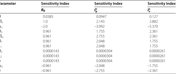
Table 2 Sensitivity indices ofR0,I∗h, andI∗v, based on the parameter values given in Table 1
Parameter Sensitivity Index Sensitivity Index Sensitivity Index
R0 I∗h I∗v
Table 1 for the model. The sensitivity indices analysis identifies the parameters that are more pivotal for disease transmission and prevalence.
Definition The normalized forward sensitivity index of a variablehthat depends on the differentiability with respect to a parameter lis defined asγlh= ∂h
∂l × l
h. The sensitivity indices ofR0,Ih∗, andIv∗are given in Table 2.
By the analysis of sensitivity indices the most sensitive parameter isμv. The reproduc-tion number R0 is inversely connected toμv. Thus, it can be said that an increase (or decrease) inμvby 10%,R0decreases (or increases) by 20%. Similarly if we increase (or decrease)σby 10%, thenR0will also decrease (or increase) by 10%.
The endemic level of infected pine trees is inversely related to the mortality rate of bark beetles and exploitation rate of infected pine trees. We see thatIh∗is decreased (increased) by almost four times with respect to the parameterμv, and it is decreased (increased) almost 27%by increasing (decreasing) the exploitation rate by 10%.
(increased) by almost five times with respect to the parameterμv, and it is decreased (in-creased) almost 23%by increasing (decreasing) the exploitation rate by 10%.
The sensitivity indices ofR0,Ih∗, andIv∗proposed that three controls, nematicide injected into the trunk of uninfected trees, cutting down infected trees burning and burying, and spray of insecticides, can be applied for vector control.
6 Optimal control analysis
Now model (1) is modified to evaluate the effect of few control measures, namely nemati-cide injected into the trunk of uninfected trees, exploiting and burying infected pine trees, and spray of insecticides. In the pine population, the factor 1 –u1is involved to reduce the associated force of infection, and the exploitation rate of infected pine trees is increased at a rateu2. The reproduction rate of the beetle population is reduced through the factor 1 –u3.
The control functionu1represents the use of nematicide injected into the trunk of unin-fected trees. The control functionu2represents the increase in exploitation rate of infected pine trees so that bark beetle could not oviposit on them. The level of adulticide used for vector control such as aerial spraying of pesticide is represented by the control functionu3. Thus the reproduction rate of the vector population is diminished by a factor of 1 –u3. Further, we assume that the exploitation rate of infected pine trees and the mortality rate of the vector population increase at rates proportional tor1andr0, respectively.
For the disease control, it is necessary to examine the optimal level of efforts. For this purpose, we design the objective functionalJ. This objective functional helps us in min-imizing the number of infected pines and also the expense of applying the controlsu1,
u2,u3: tryagin’s maximum principle [15] is used to satisfy the necessary conditions of the optimal solution. For the application of this principle, we define the HamiltonianHas
+λ2
Hereλi,i= 1, 2, 3, 4, are the adjoint variables. To prove the existence of the optimal con-trol using the result given by Fleming and Rishel [16], we state and prove the following theorem.
Theorem 6.1 There exists an optimal control(u∗1,u∗2,u∗3)that minimizes J over U subject to the control system(11).Further,for system(11),there exist adjoint variablesλi,i= 1, 2, 3, 4,
satisfying Since the state solutions are bounded, the state system satisfies the Lipschitz property corresponding to the state variables. The existence of optimal control follows from [16]. The equations representing the rate of change of the adjoint variables are formed by the differentiation of the Hamiltonian function with respect to state variables evaluated at the optimal control. The optimal solution given by (15) can be obtained by solving the equations
on the internal of the control set using the property of the control spaceU.
7 Numerical simulations
Figure 1 The Population approaches disease-free equilibrium whenR0< 1.
Figure 2 The Population approaches endemic equilibrium whenR0> 1.
whereas Figure 2 shows that the population approaches endemic equilibrium as the re-production number exceeds unity.
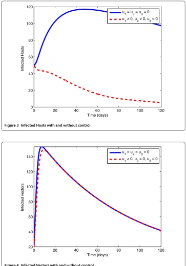
Now, we investigate numerical results for the efficacy of the optimal control planning for the disease spread in a community. We have chosen the set of weight factorsA1= 1,
A2= 5,B1= 3,B2= 7,B3= 9 and initial state variablesSh(0) = 100,Ih(0) = 50,Sv(0) = 150,
Figure 3 Infected Hosts with and without control.
Figure 4 Infected Vectors with and without control.
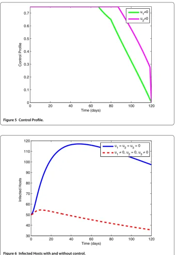
7.1 Application of preventive measures (u1= 0) and exploiting and disposing off
infected pines (u2= 0)
Figure 5 Control Profile.
Figure 6 Infected Hosts with and without control.
strategy to control the number of infected vectors. The control profile explored in Figure 5 states that the controlu1remains at the upper bound till 35 days, whereas the controlu2 rises to the upper bound after 60 days.
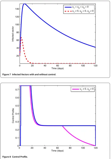
7.2 Application of preventive measures (u1= 0) and spray of insecticides (u3= 0)
Figure 7 Infected Vectors with and without control.
Figure 8 Control Profile.
of infected pines and infected vectors, respectively. By the analysis of control profile shown in Figure 8 we see that the controlu1rises to its upper bound in 20 days, and after these days it gradually drops down to zero, whereas the controlu3can be activated after 20 days.
7.3 Use of exploitation of infected pines (u2= 0) and spray of insecticides (u3= 0)
Figure 9 Infected Hosts with and without control.
Figure 10 Infected Vectors with and without control.
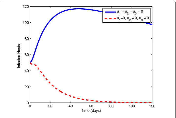
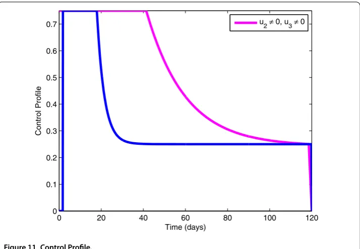
7.4 Use of preventive measures (u1= 0), exploitation of infected pines (u2= 0) and spray of insecticides (u3= 0)
Figure 11 Control Profile.
Figure 12 Infected Hosts with and without control.
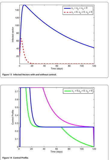
7.5 Effects of weight constants
Figure 13 Infected Vectors with and without control.
Figure 14 Control Profile.
Competing interests
The authors declare that they have no competing interests.
Authors’ contributions
All authors carried out the proofs of the main results and approved the final manuscript.
Author details
1Department of Mathematics, University of the Punjab, Lahore, Pakistan.2Department of Mathematics, COMSATS
Figure 15 Plot of different weight constants on the controlu1.
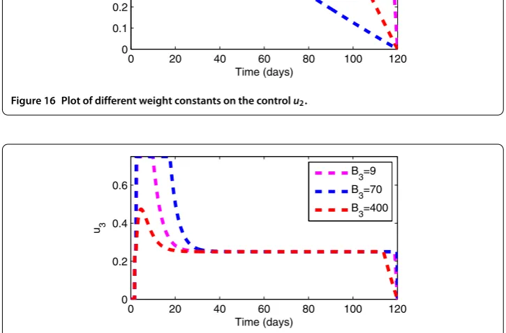
Figure 16 Plot of different weight constants on the controlu2.
Figure 17 Plot of different weight constants on the controlu3.
Publisher’s Note
Springer Nature remains neutral with regard to jurisdictional claims in published maps and institutional affiliations.
Received: 10 October 2017 Accepted: 12 January 2018
References
1. Ozair, M, Lashari, AA, Jung, IH, Okosun, KO: Stability analysis and optimal control of a vector-borne disease with nonlinear incidence. Discrete Dyn. Nat. Soc.2012, Article ID 595487 (2012).
2. Yoshimura, A, Kawasaki, K, Takasu, F, Togashi, K, Futai, K, Shigesada, N: Modeling the spread of pine wilt disease caused by nematodes with pine sawyers as vector. Ecology80(5), 1691-1702 (1999)
4. Edwards, OR, Linit, MJ: Transmission of Bursaphelenchus xylophilus through oviposition wounds of Monochamus carolinensis (Coleoptera: Cerambycidae). J. Nematol.24, 133-139 (1992)
5. Ozair, M, Shi, X, Hussain, T: Control measures of pine wilt disease. Comput. Appl. Math. (2014). https://doi.org/10.1007/s40314-014-0203-2
6. Li, MY, Muldowney, JS: A geometric approach to global stability problem. SIAM J. Math. Anal.27, 1070-1083 (1996) 7. Buonomo, B, Vargas-De-Leon, C: Stability and bifurcation analysis of a vector-bias model of malaria transmission.
Math. Biosci.242(1), 59-67 (2013)
8. Tumwiine, J, Mugisha, JYT, Luboobi, LS: A host vector model for malaria with infective immigrants. J. Math. Anal. Appl.
361(1), 139-149 (2010)
9. Lee, KS: Stability analysis and optimal control strategy for prevention of pine wilt disease. Abstr. Appl. Anal.2014, Article ID 182680 (2014)
10. Togashi, K: Population density of Monochamus alternatus adults (Coleoptera: Cerambycidae) and incidence of pine wilt disease caused by Bursaphelenchus xylophilus (Nematoda:Aphelenchoididae). Res. Popul. Ecol.30(2), 177-192 (1988)
11. Monserud, RA, Sterba, H: Modeling individual tree mortality for Austrian forest species. For. Ecol. Manag.113(2-3), 109-123 (1999)
12. Kim, DS, Lee, SM, Huh, HS, Park, NC, Park, CG: Escape of pine wood Nematode, Bursaphelenchus xylophilus, through feeding and oviposition behavior of Monochamus alternatus and M.saltuarius (Coleoptera: Cerambycidae) adults. Korean J. Appl. Entomol.48(4), 527-533 (2009)
13. Kobayashi, F, Yamane, A, Ikeda, T: The Japanese pine sawyer beetle as the vector of pine wilt disease. Annu. Rev. Entomol.29, 115-135 (1984)
14. Kim, DS, Lee, SM, Kim, CS, Lee, DW, Park, CG: Movement of Monochamus altermatus hope (Coleoptera: Cerambycidae) adults among young black pine trees in a screen cage. Korean J. Appl. Entomol.50(1), 1-6 (2011) 15. Pontryagin, LS, Boltyanskii, VG, Gamkrelidze, RV, Mishchenko, EF: The Mathematical Theory of Optimal Processes, vol.
4. Gordon & Breach, New York (1986)