R E S E A R C H
Open Access
Modelling the guaranteed QoS for wireless sensor
networks: a network calculus approach
Lianming Zhang
1*, Jianping Yu
2and Xiaoheng Deng
3Abstract
Wireless sensor networks (WSNs) became one of the high technology domains during the last 10 years. Real-time applications for them make it necessary to provide the guaranteed quality of service (QoS). The main contributions of this article are a system skeleton and a guaranteed QoS model that are suitable for the WSNs. To do it, we develop a sensor node model based on virtual buffer sharing and present a two-layer scheduling model using the network calculus. With the system skeleton, we develop a guaranteed QoS model, such as the upper bounds on buffer queue length/delay/effective bandwidth, and single-hop/multi-hops delay/jitter/effective bandwidth. Numerical results show the system skeleton and the guaranteed QoS model are scalable for different types of flows, including the self-similar traffic flows, and the parameters of flow regulators and service curves of sensor nodes affect them. Our proposal leads to buffer dimensioning, guaranteed QoS support and control in the WSNs.
Keywords:wireless sensor networks, quality of service, network calculus, upper bounds
1. Introduction
Wireless sensor networks (WSNs) have been became one of the high technology domains of the seven seas, and theoretic and applications study about them are more and more regarded in recent years [1-3]. Real-time application areas for the WSNs encompass tracking, environment scouting, fo-recasting and medical care. Sink nodes of the WSNs respond in time on needs, so data channel between sink nodes and sensor nodes must offer a guaranteed quality of service (QoS). It includes deterministic sending rate, transmission with-out loss, end-to-end delay with upper bound and so on [1]. The guaranteed QoS plays an important role in data transmission for the WSNs. For example, the end-to-end delay with upper bound is one of the guaranteed services, whether the upper bound on end-to-end can obtain a guarantee is a key to provide the guaranteed QoS and to complete effectively routing, congestion control and load balancing. To fulfill aims, the WSNs need to send some special probe packets [4]. The extra cost accounts for much total power under constrained energy, bandwidth and buffer size of a sensor node.
However, it results in shortening of the WSNs’lifetime, and it is important to provide the guaranteed QoS model and the performance evaluation method for the WSNs.
Network calculus is a set of recent developments that enable the effective derivation of deterministic perfor-mance bounds in networking [5,6]. Compared with some traditional statistic theories, network calculus has the merit that provides deep insights into performance analysis of deterministic bounds. Now, research areas for the network calculus include mostly QoS control, resource allocation and scheduling, and buffer/delay dimensioning in the virtual circuit switched networks, the guaranteed service networks and the aggregate sche-duling networks [5].
In recent years, the end-to-end delay bounds, in FIFO-multiplexing tandems, were esti-mated based on the least upper delay bound (LUDB) method [7]. The delay of individual traffic flows, in feed-forward networks under arbitrary multiplexing, was computed [8]. The maximum end-to-end delay, for a given flow in any feed-forward network under blind multiplexing, was cal-culated [9]. Resource allocation and congestion control was investigated in distributed sensor networks using the network calculus [10]. An analytical framework was presented, based on the network calculus, to analyse * Correspondence: [email protected]
1
College of Physics and Information Science, Hunan Normal University, Changsha, Hunan 410081, China
Full list of author information is available at the end of the article
worst-case performance and to dimension resources of sensor networks [11-14]. The power management pro-blem in video sensor networks was investigated [15]. The worst-case performance of the WSNs was analysed [16]. Recently, the cluster-tree WSNs were modelled and dimensioned in the network calculus [17-19].
In previous studies [20-23], we drawn the determinis-tic performance bound on end-to-end delay jitter for self-similar traffic regulated by a fractal leaky bucket regulator in a generalized processor sharing system, and obtained the deterministic and statistical performance bounds on end-to-end delay in the WSNs and the wire-less mesh networks.
In this article, we describe a generalized scenario of the WSNs, and present a practicable model of sensor nodes for guaranteed service support using a scheme based on virtual buffer sharing. On the basis of the notion of flows and microflows, we propose, using arri-val curves and service curves in the network calculus, a two-layer scheduling model for sensor nodes. We develop a guaranteed QoS model, including the upper bounds on buffer queue length/delay/effective band-width, and single-hop/multi-hops delay/jitter/effective bandwidth. Combined with the research results of pre-decessor researchers, the main different contributions of this study are as follows. First, we present a system ske-leton and a guaranteed QoS model that are suitable for the WSNs with some characteristics of distribution and multi-hops, and the sensor node model which not only fulfills these wants, but also makes performance analysis simpler. Second, we find that quantitative relations between the upper bounds on buffer queue length/ delay/effective bandwidth, and single-hop/multi-hops delay/jitter/effective bandwidth and the service rate, the latency of the service curves in sensor nodes, and as well as the hops. Third, we reveal the impact of the ser-vice rate, the latency and the parameters of the regula-tors, including the Hurst parameter of self-similar traffic flows, on the guaranteed QoS. The findings’ contribu-tions are used to modelling the guaranteed QoS for the WSNs, and they may have potential applications to buf-fer and delay di-mensioning, QoS support, routing implementing, congestion control and load balancing for the WSNs and other wireless networks with some char-acteristics of distribution and multi-hops.
The rest of the article is organized as follows. Section 2 devotes to the background knowledge of the network calculus. Section 3 discusses a system skeleton, includ-ing a generalized scenario of the WSNs, a sensor node model, the flow source model, the guaranteed QoS ser-vice and the scheduling model of a sensor node. Section 4 draws the upper bounds on the guaranteed QoS model. Section 5 shows the numerical results and com-pares one another to demonstrate the availability and
the merits of the proposed skeleton, the guaranteed QoS model and our approach through same examples. Finally, Section 6 contains the summary of the results, some inferring remarks and future works.
2. Background on network calculus
In this section, we provide a brief background on the network calculus used in the article. Network calculus is the results of the studies on traffic flow problems, min-plus algebra and max-min-plus algebra applied to qualitative or quantitative analysis for networks in recent years, and it belongs to tropical algebra and topical algebra.
Network calculus can be classified into two types: deterministic network calculus and statistical network calculus. The former, using arrival curves and service curves, is mainly used to obtain the exact solution of the bounds on network performance, such as queue length and queue delay, and so on. And then the latter, based on arrival curves and effective service curves, is used to obtain the stochastic or statistical bounds on the network performance. Here, we give only the neces-sary introductory material used in this article.
Theorem1 (queue length and queue delay): Assume a flow passes through a sensor node, and the sensor node has an arrival curve a(t) and offers a service curveb(t). The queue lengthQand the queue delayDof the flow, passing through the sensor node, satisfy, respectively,
Q≤supt≥0{α(t)−β(t)}, (1) and
D≤inft≥0{d≥0 :α(t)≤β(t+d)}. (2) Theorem2 (multi-hops service curve): Assume a flow passes through the sensor node 1, node 2, ..., nodeNin sequence. Assume the sensor nodes offer the service curves ofb(1), b(2), ...,b(N)to the flow, respectively. The fixed delays between two neighbor sensor nodes ared1, d2, ..., dN-1 in sequence. The multi-hops service curve bm-hsatisfies
βm−h =β(1)⊗β(2)⊗ · · · ⊗β(N)⊗δ
d1+···+dN−1, (3)
where⊗is the operator of the min-plus convolution given by
(f⊗g)(t) =
infs∈[0,t][f(t−s) +g(s)], t≥0
0, t<0 ,
andδd is called a burst delay function. For 0≤t≤ d,
δd(t) = 0, and fort>d,δd(t) = +∞.
In Equation 3, we obtain, settingn= 2, the single-hop service curvebs-has follows
The proof of the theorems and more information about the network calculus are found in [5,6].
3. System skeleton
3.1. System model
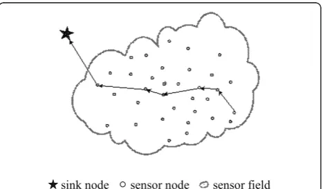
In the following, we firstly describe a generalized sce-nario of the WSNs, where includes sink nodes, sensor nodes and a sensor field as shown in Figure 1.
When certain sensor node of the sensor field probes an occurring event, the sensor node sends probed data to one of its neighbor sensor nodes according to the route arithmetic arranged in advance, and then the neighbor sensor node sends the data to one of its neigh-bor sensor nodes. Finally, the data probed by the first sensor node is transmitted to a sink node passing multi-hops.
In general, the energy of a sensor node is supplied by battery under constrained energy, so the storage and communication capacity of a sensor node is constrained. It is essential to provide the guaranteed QoS to lessen spending and to prolong a network lifetime.
The next, we present, using a scheme based on virtual buffer sharing, a sensor node model as shown in Figure 2. The buffer of the sensor node is allocated to data channels between the sensor node and its upstream neighbor nodes. The probed data from its upstream neighbor nodes share the buffer of the sensor node. The scheduler of the sensor node sends the data to the downstream neighbor nodes according to the QoS priority. Figure 2 shows the case for the sensor node j and i upstream neighbor nodes, including the sensor node 1, node 2, ..., nodei.
Remark 1: The sensor node model using the virtual buffer sharing has some merits as follows.
(1) The model provides a minimum guaranteed ser-vice rate for every data channel from upstream neighbor nodes under constrained bandwidth,
namely, when the data flow passes through a sensor node, the node guarantees a minimum service rate. (2) The buffer and the bandwidth of a sensor node are shared by all of upstream neighbor nodes and delivered to them in part to their weights, so the WSNs obtain a larger gain from the statistical multi-plexing of independent flows.
(3) The model makes performance analysis simpler, and it is suitable for mobile sensor nodes in the WSNs.
3.2. Flow source model
The dynamic and complexity properties of the network and the fluctuation of the traffic possibly cause the bur-stiness of the traffic flows in the WSNs. They increase the average delay and result in the unfairness of resource allocation. It becomes more difficult in provid-ing or analysprovid-ing the guaranteed QoS. In this article, we can categorize traffic flows into two types: flow and microflow. The former contains file flows, audio flows and video flows and so on. The latter, belonging to the identical type, aggregates a flow. The aggregate flow enters a sharing buffer to queue and schedule for the sensor node. In this article, we select the leaky bucket source model due to its simplicity and practical applic-ability, and use leaky bucket regulators to regulate the microflows at every sensor node, to enable non-rule microflows to be restraint under the certain conditions. The microflow, regulated by the leaky bucket regulator, is indicated by envelopea(t) as shown in Equation 4,
α(t) = min m∈{1,...,M}{r
m·t+bm},∀t≥0,
(4)
where the case of M = 1 agrees to the simple leaky bucket regulator,bis interpreted as the burst parameter, andr as the average arrival rate.
Remark 2: the microflow in an interval [t, t+τ] is denoted byA(t,t+τ), and it has the following properties as shown in [24].
sink node sensor node sensor field
Figure 1A generalized scenario of WSNs.
virtual queue 1 sensor node 1
sensor node 2
sensor node i
virtual queue 2
virtual queue i sensor node j
scheduler
Property1 (additivity):
A(t1,t3) =A(t1,t2) +A(t2,t3),∀t3>t2>t1>0. Property2 (sub-additive bound):
A(t,t+τ)≤α(τ),∀t≥0,∀τ ≥0.
Property 3 (independence): all microflows are independent.
3.3. Guaranteed QoS
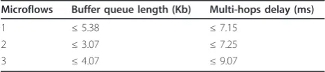
The guaranteed QoS provides the QoS guarantees which involve the stability of performance, the usability and reliability of calculation resources, as well as the rationality of calculation price. In this article, we mainly discuss how to provide guarantees for the QoS, including the upper bounds on buffer queue length/ delay/effective bandwidth, and the upper bounds on single-hop/multi-hops delay/jitter/effective bandwidth. It is important to limit the values of buffer queue length/delay/jitter to a sustainable level below the upper bounds. For example, once the value of tracking or environment scouting delay is beyond a certain value, such as the upper bound on end-to-end delay in the WSNs, the accuracy of tracking and the effective-ness of environment scouting have sharply declined. Table 1 reports an example of guaranteed service that comes from the experimental results for a real-time tracking environment and scouting application in the cluster-tree WSNs based on IEEE 802.15.4/ZigBee pro-tocol in [19].
3.4. Two-layer scheduling model
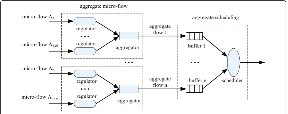
In the following, we present a two-layer scheduling model of a sensor node as shown in Figure 3. The pro-cess of the model is as follows: First, the microflows, entering a sensor node, with the same or similar QoS are regulated by a leaky bucket regulator given in Equa-tion 4, and serves for the arrival curvea(t) of the next buffer. The functionsa(t) andA(t,t+τ) satisfy Property 2; Second, we assume that the first come, first served strategy is adopted in the buffer, and the microflows, belonging to the same type, enter a special buffer assigned by the sensor node; Finally, the aggregate flows are scheduled in a way of a service curveb(t). The ser-vice curve is shown as follows.
From Properties 1 and 3, and Figure 3, the aggregate flows Aj(t, t+τ) and microflows Aj,k(t, t+τ), k= 1,2,...,n satisfy
Aj(t,t+τ) =
n
k=1Aj,k(t,t+τ), ∀t,τ >0 (5) From [25], the equivalent envelope curve aj(t) of the aggregate flows and the envelope curveaj,k(t) (k= 1,2,..., n) of the microflows satisfy
αj(t) =
n
k=1αj,k(t), ∀t>0. (6)
The service curvebi(t) of the flowiis defined as
βi(t) =β(t)− n
k=1,k=i
αk(t−θk), ∀t> θ≥0, (7)
whereb(t) is interpreted as a service curve of sensor node,akas an arrival curve of the bufferk, andnas the number of the buffers in the sensor node.
In order to simplify the calculation, without loss of generality, we assume the service curveb(t) of the sen-sor node is a rate-latency functionbR,T(t) given by
β(t) =βR,T(t) =R·(t−T),∀t>T>0, (8) whereRis interpreted as the service rate,Tas the latency. Obviously forR> 0 and 0≤t≤T, we havebR,T(t) = 0.
From Property 3, Equations 5 and 6, the simple leaky bucket regulator is used, and the envelope curve of the regulator is
αi(t) =εi(t) =
n
k=1(bi,k+ri,kt). (9) From Equations 4 and 8, ifni=1ri<R, then the para-meterθiis optimized, and we have
θi=T+ n
k=1,k=i
bk/R, i= 1, 2, . . ., n
Substituting θiinto Equation 7, and combining Equa-tion 6 with EquaEqua-tion 9, we obtain
βi(t) =
⎛ ⎝R−
n
k=1,k=i cj
j=1 rk,j
⎞ ⎠·
⎛ ⎝t−T−
n
k=1,k=i cj
j=1 bk,j/R
⎞
⎠. (10)
Remark 3: From Equation 10, we have known, each flow, which enters the sensor node scheduler, holds a certain service curve, and the service curve will not only be decided by the total service curve of the sensor node scheduler, but also by the arrival curve of the flow.
4. Guaranteed QoS model
In this section, we present, using the network calculus, the guaranteed QoS model. The model is mainly used in
Table 1 An example of the guaranteed QoS
Microflows Buffer queue length (Kb) Multi-hops delay (ms)
1 ≤5.38 ≤7.15
2 ≤3.07 ≤7.25
two aspects: one is the off-line dimensioning of a sys-tem, which is responsible for the quantification to obtain the pre-arranged resources providing the guar-anteed QoS; and the other is the on-line admission control, which is responsible to decide whether receives a new flow according to the QoS requirements and the usable resources. In the following, the guaran-teed QoS model, including the upper bounds on Qi, Di, ei, DDN, ΔDN and eeN (in Table 2) of the system skeleton in Section 3 are discussed in the network calculus.
4.1. Node QoS model
Proposition1: (upper bound on buffer queue length): In an interval [0,t], the upper bound onQisatisfies
Qi= supt≥0
Proof: From Equation 1, we have
Qi≤supt≥0{αi(t)−βi(t)}. (12)
Substituting Equations 9 and 10 into Equation 12, we hold
Proposition2: (upper bound on buffer queue delay): In an interval [0,t], the upper bound onDisatisfies
Di=T+
Proof: From Equation 2, we obtain
Di≤inft≥0{d≥0 :αi(t)≤βi(t+d)}. (14) Substituting Equations 9 and 10 into Equation 14, we have
Figure 3Two-layer scheduling model.
Table 2 The parameters of the QoS
Symbol Definition
Qi Buffer queue length of the sensor nodei Di Buffer queue delay of the sensor nodei
ei Buffer queue effective bandwidth of the sensor nodei DDN Single-hop delay forN= 2, and multi-hops delay forN> 2
ΔDN Single-hop delay jitter forN= 2, and multi-hops delay jitter forN> 2
Proposition 3: (upper bound on buffer effective bandwidth): In an interval [0,t], the upper bound onei satisfies
whereDiis given by Equation 13.
Proof: Substituting Equation 9 into Equation 1.30 in [5], we have Equa-tion 16.
Remark 4: The leaky bucket regulators and aggrega-tors do not increase the upper bounds on buffer queue length/delay/effective bandwidth of a sensor node, and also do not increase the buffer requirements of the sensor node.
4.2. Single-hop and multi-hops QoS model
Proposition4: (upper bound on single-hop and multi-hops delay): Assume a flow passes through the sensor node 1, node 2, ..., node Nin sequence, and the sensor node i offers the service curves ofb(1), b(2), ...,b(N)to the flow, respectively. The fixed delays between two neighbor sensor nodes are d1, d2, ...,dN-1 in sequence. The upper bound onDDNsatisfies
DDN =T1+
whereRiandTi are interpreted as the service rate and the latency of the sensor nodei, andr(ki,)j andb(ki,)jas the burst parameter and the average arrival rate of the leaky bucket regulator of the sensor nodei, respectively.
Proof: From Equations 10, 3 and 8, we hold
βm−h
Substituting Equations 9 and 18 into Equation 2, we have Equation 17.
Proposition5 (upper bound on single-hop and multi-hops delay jitter): Assume a flow passes through the sensor node 1, node 2, ..., nodeNin sequence, and the sensor nodeioffers the service curves of b(1), b(2), ...,b (N) to the flow, respectively. The fixed delays between
two neighbor sensor nodes are d1, d2, ..., dN-1 in sequence. The upper bound onΔDNsatisfies
DN=T1+
whereT1is interpreted as the latency of the first sen-sor node,b(1)i,k as the burst parameter of the microflowk of the flowi, entering the first sensor node, and others in Equation 19 are shown in Equation 17.
Proof: The upper bound onDDNobtained from Equa-tion 17 is the total delay, and the upper bound onΔDN and the fixed delay Dc hold ΔDN = DDN - Dc. The multi-hops fixed delay is defined as Dc=
N−1 i=1 di. Therefore, Equation 19 exists obviously.
Proposition6 (upper bound on single-hop and multi-hops effective bandwidth): Assume a flow passes through the sensor node 1, node 2, ..., node N in sequence, and the sensor nodeioffers the service curves of b(1),b(2), ..., b(N)to the flow, respectively. The fixed delays between two neighbor sensor nodes ared1,d2, ..., dN-1in sequence. The upper bound oneeNsatisfies
eeN= max
where the parameters in Equation 20 are given in Equation 19.
Proof: From Equations 9 and 16, we obtain
eeN≤max{ri,k,bi,k
Di,k},
for Di,k ≥ Di, from Equations 17 and 16, we have Equation 20.
Remark5: The single-hop scenario is a special case of the multi-hops WSNs. In Equations 17, 19 and 20, we obtain the single-hop QoS model forN= 2, and obtain the multi-hops QoS model forN> 2.
Remark 6: The leaky bucket regulators and aggrega-tors do not increase the upper bounds on single-hop/ multi-hops delay/jitter/effective bandwidth of the WSNs.
5. Numerical results
the latency of the service curves of the sensor nodes. The fixed delay between two neighbor sensor nodes is marked asd.
Figure 4 shows the transmission of three flows in the WSN. The three flows, namely, flow1, flow2 and flow3, are marked as A1(t), A2(t) andA3(t), respectively. They come from the sensor nodes A, B and C. Hence, with-out any loss of generality, we assume the flowA1(t) con-tains three microflows:A1,1(t),A1,2(t),A1,3(t), the flowA2 (t) contains two microflows:A2,1(t) andA2,2(t), and the flowA3(t) contains one microflow:A3,1(t).
Recent research suggests that the sensory data flow is bounded by arrival curvea(t) = 576(bps) + 390(b) xtin the cluster-tree WSNs based on IEEE 802.15.4/ZigBee protocol in [19]. Here, we consider the case of M= 2 in Equation 4 and assume that every microflow is regulated by the leaky bucket regulatora(t) as shown in Equation 9. The average arrival rateri,kand the burst tolerance bi,
kof the six microflows are shown in Table 3. Obviously, the arrival curves of the flows are given by Equation 10.
Remark7: The units of buffer queue lengthQ, effec-tive bandwidth e and ee are Mb, the units of delayD andDD, the time t, the latencyTand the fixed delay d are ms and the unit of the service rateRis Mbps except the units that are given.
5.1. Node QoS
In the following, we discuss the relations between the sensor node QoS and the parameters of the service curve provided by the sensor nodes, and the time evolu-tion of the sensor node QoS.
Figure 5 shows the impact of the service rateR and the latency T on the upper bounds on buffer queue lengthQand the evolution laws ofQin a sensor node. We see a straightforward dependency: the upper bound
onQis smaller for smaller service rateRwith low-value or smaller latencyT; it is smaller for larger service rate R with high-value or larger evolution time t. For all flows, the changing tendency of the upper bound onQ with the increase of the service rateRor the latency T and the time evolution tof Qare the same. The size deviation of the upper bounds on Q1, Q2andQ3 of the flows: A1(t),A2(t) and A3(t) is equal regardless of R values and Tvalues. The upper bound on Q2ofA2(t) is more than that ofQ1 ofA1(t), and that ofQ3 of theA3
1 2 N-1 N
A
B
C
Figure 4General scenario of WSNs.
Table 3 The parameters of the three flows
FlowsAi(t) Mico-flows
Ai,k(t)
Average arrival rateri,k(Kbps)
Burst tolerance
bi,k(Kb)
A1(t) 1 500 30
2 300 300
3 420 150
A2(t) 1 600 200
2 240 500
A3(t) 1 300 200
0 1 2 3 4 5
x 105 1400
1600 1800 2000 2200 2400
Service Rate ( R )
UBBQL (
Q )
(a) flow1
flow2 flow3
0 0.002 0.004 0.006 0.008 0.01 0.012
1000 1500 2000 2500 3000 3500
Latency ( T )
U
B
B
Q
L
( Q
)
(b) flow1
flow2 flow3
0 0.002 0.004 0.006 0.008 0.01
500 1000 1500 2000 2500
Time ( t )
UBBQL (
Q )
(c) flow1
flow2 flow3
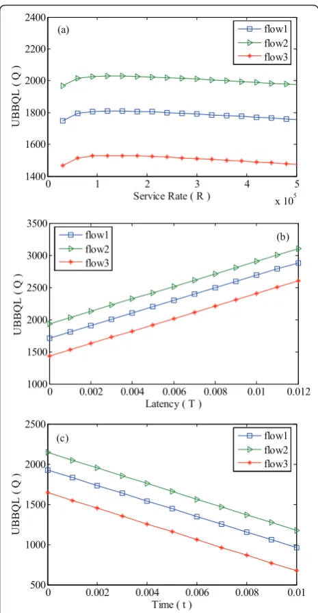
Figure 5The upper bounds on buffer queue length (UBBQL)Q (in Kb) of a sensor node:(a)Qas a function of the service rateR
(in Kbps) forT= 1 andt= 1.2;(b)Qas a function of the latencyT
(t) is smallest. Obviously, the impart of the latencyT or burst tolerance b on the upper bound on Q is more than that of the service rateRor the average arrival rate r, respectively.
Figure 5a plots the Qcurves as a function of the ser-vice rateR. The upper bound on Qfor any flow reaches a maximum Qmax when the service rate R = 128, and the Qmax value of the flows: A1(t), A2(t) and A3(t) is 1.81, 2.03 and 1.53, respectively. The shapes of curves at the two sides of the maximum point are asymmetric. For example, at the distance 50 from the maximum point on the left, the Qmax value of the three flows is 1.81, 2.02 and 1.52, but the Qmax value of the three flows is 1.81, 2.03 and 1.53, respectively, at the same dis-tance on the right.
Figure 5b plots the Q curves as a function of the latency T. The upper bound on Q increases linearly with the increase of the latencyT, and the slope of each line is 9.764 × 10⁴.
Figure 5c plots theQcurves as a function of the evo-lution time t. There exists a linear relationship between the upper bound onQand the evolution timetand the same slopes of the all lines are -9.642 × 10⁴.
Figure 6 shows the impact of the service rateR and the latency T on the upper bounds on buffer queue delay D in a sensor node. We see a straightforward dependency: the upper bound on Dis smaller for larger service rateR; it is smaller for smaller latencyT.
Figure 6a plots the Dcurves as a function of the ser-vice rate R. TheDvalues, curving inwards, decay with the increase of Rregardless ofT values, nearly conver-ging 0 for all flows. The decay rates in the upper bounds onDby the near exponential increase with the increase of the service rateRfor certain flow, and increase with the increase of the burst toleranceb of the flows with the same service rate T. For instance, if T= 1 andR= 50, then the Dvalue of the flows:A1(t),A2(t) andA3(t) is 38.7, 43.3 and 32.8, and if T = 1 and R= 200, then the D value of the three flows is 10.3, 11.4 and 8.9, respectively.
Figure 6b plots the D curves as a function of the latencyT. The upper bounds onDincrease linearly with the increase of the latency Tregardless of theRvalues. The slopes of all lines are 1.
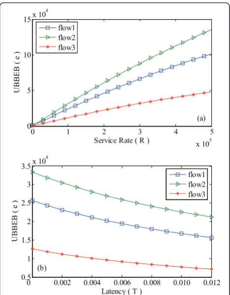
Figure 7 shows the impact of the service rateR and the latency T on the upper bound on buffer effective bandwidthe in a sensor node. We see a straightforward dependency: the upper bound on e is larger for larger service rateR; it is larger for smaller latencyT.
Figure 7a plots an ecurve as a function of the service rate R. The e values increase with the increase of R values, and the increase rate is getting smaller and smal-ler with the increase ofRvalues for certain flow regard-less of the values of the latencyT. The delay rates of the
increase rates decrease with the increase of the burst tolerance b of the flows. For instance, ifT = 1 andR= 50, then theevalue of the flows: A1(t),A2(t) andA3(t) is 12.41, 16.17 and 6.10, and if T = 1 and R= 200, then theevalue of the three flows is 46.47, 61.18 and 22.44, respectively.
Figure 7b plots an ecurve as a function of the latency T. The upper bounds onedecrease with the increase of Tvalues, and the decay rate is getting smaller and smal-ler with the increase ofTvalues for certain flow regard-less of theR values. Thee curves of all flows are near parallel.
In summary, the performance curves denote the upper bounds of the sensor node QoS. In Figures 5, 6 and 7, the curves show the deterministic worst-case length/ delay/effective bandwidth in the buffer queue of a sensor node, respectively. It means that the values of the buffer queue length/delay must are lower than the values of the performance curves. We can reduce, regulating the average arrival rater and the burst tolerance b of the microflows by controlling the parameters of the regula-tors or regulating the service rate Ror the latencyT of a sensor node by controlling the parameters of the sche-duler, the values of the upper bounds on buffer queue
0 1 2 3 4 5
x 105 0
0.02 0.04 0.06 0.08
Service Rate ( R )
UBBQD (
D )
(a)
flow1 flow2 flow3
0 0.002 0.004 0.006 0.008 0.010 0.012 0.015
0.020 0.025 0.030 0.035 0.040
Latency ( T )
UBBQD (
D )
(b) flow1
flow2 flow3
length/delay of a sensor node to achieve these purposes that the buffer queue length/delay is very small. Instead, we can increase, regulating the average arrival raterand the burst toleranceb or regulating the service rateRor the latencyT, the value of the upper bound on buffer queue effective bandwidth to obtain a guaranteed band-width for those flows through the sensor node, and eventually reduce the buffer queue delay.
5.2. Multi-hops and single-hop QoS
In the following, we discuss the relations between the multi-hops QoS and the single-hop QoS and the para-meters of the service curve provided by the sensor nodes and the hops. We still use the general scenario of WSNs as known in Figure 4.
5.2.1. The case 1
The sensor nodes (node 1, node 2, ..., node N-1, node N) have the same service curves:b1(t) = b2(t) = ... =b N-1(t) = bN(t) =b(t) =R(t-T). From Equation 8, we have R1 =R2 = ... =RN-1=RN=R, andT1 =T2 = ... =TN-1 =TN =T. To make easy the following discussion, we assume that the fixed delays between two neighbor sen-sor nodes are the same: d1 =d2 = ... = dN-1 =d. First,
we investigate the multi-hops scenario with hops higher than 2.
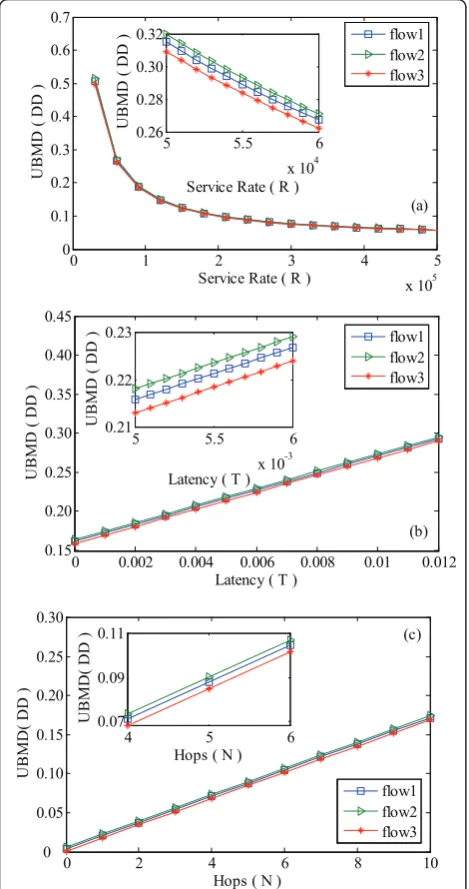
Figure 8 shows the impact of the service rate R, the latency T and the hops N on the upper bounds on multi-hops delay DD. We see a straightforward depen-dency: the upper bound on DDis smaller for larger ser-vice rate R; it is smaller for smaller latency T and smaller hopsN.
Figure 8a plots aDD curves as a function of the ser-vice rateR. TheDD values, curving inwards, decay with the increase ofRregardless ofT values,Nvalues andd values for certain flow. The decay rates in the upper bounds on DD by the near exponential increase with the increase of the service rate Rfor certain flow, and increase slightly with the increase of the burst tolerance b of the flows for the sameT. For instance, ifT1 =T2= ... =TN-1 =TN=T = 1,R1=R2= ... =RN-1 =RN=R= 50, d1 = d2 = ... = dN-1 = d = 2 andN = 10, the DD value of the flows:A1(t),A2(t) and A3(t) is 315, 320 and 309, and if T = 1,R= 200,d = 2, andN = 10, theDD value of the three flows is 100, 102 and 99, respectively.
Figure 8b plots a DD curves as a function of the latencyT. The upper bounds onDD increase in linear with the increasing of Tvalues regardless ofRvalues,N values and d values for certain flow. All the increase rates ofDDare 11.
Figure 8c plots aDD curves as a function of the hops N. The upper bounds onDDincrease in linear with the increase of N regardless of R values, T values and d values for certain flow. All the in-crease rates ofDDare 0.017.
Remark 8: From Equations 17 and 19, we have the relation between the multi-hops delay jitterΔDand the multi-hops delayDDas follows:ΔD=DD-Σd, whered is the fixed delay between two neighbor sensor nodes. As a result, we can obtain some numerical results about the upper bounds onΔDby setting d1=d2 = ... =dN-1 =d= 0, and the impact of the service rateR, the latency Tand the hopsNonΔDis similar to those onDD.
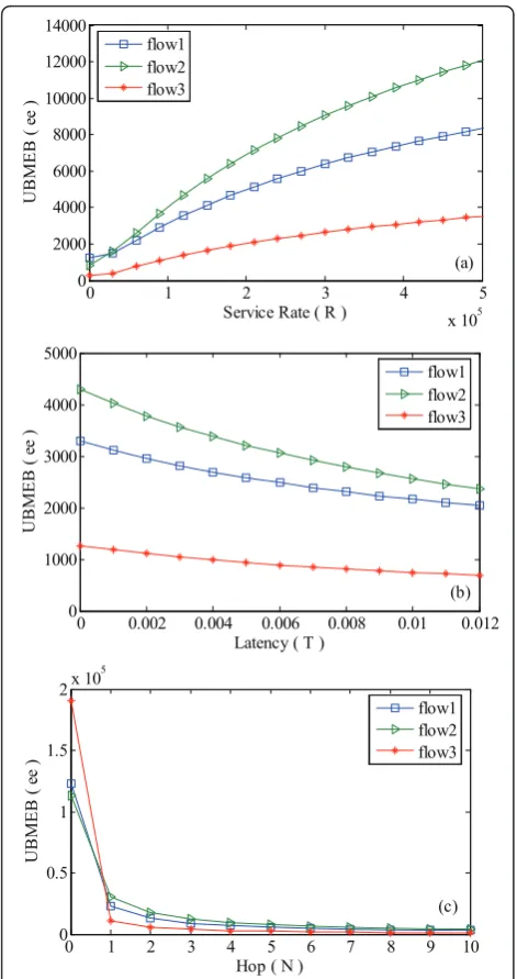
Figure 9 shows the impact of the service rate R, the latency T and the hops N on the upper bounds on multi-hops effective bandwidth ee. We see a straightfor-ward dependency: the upper bound on eeis larger for larger service rate; it is larger for smaller latency and smaller hops.
Figure 9a plots an ee curves as a function of the ser-vice rate R. The upper bounds onee increase with the increase of R values, and the increase rate is getting smaller and smaller with the increase ofR for certain flow regardless of the values of the latencyT, the fixed delayd and the hopsN. The impact of the burst toler-ance b onee is more than that of the service rateRon eefor the high-valuesR >30 or the impact of the service rate R is more. For example, ifN = 10,T = 1, R = 20
0 1 2 3 4 5
x 105 0
5 10 15x 10
4
Service Rate ( R )
UBBEB (
e
)
(a) flow1
flow2 flow3
0 0.002 0.004 0.006 0.008 0.010 0.012 0.5
1 1.5 2 2.5 3 3.5x 10
4
Latency ( T )
UBBEB (
e
)
(b)
flow1 flow2 flow3
Figure 7The upper bounds on buffer effective bandwidth (UBBEB)e(in Kb) of a sensor node:(a)eas a function of the service rateR(in Kbps) forT= 1;(b)eas a function of the latencyT
andd= 2, the eevalue of the flows:A1(t),A2(t) andA3 (t) is 1.32, 1.26 and 0.30, and ifN= 10, T= 1,R= 200 and d= 2, the eevalue of the three flows is 4.98, 6.89 and 2.02, respectively.
Figure 9b plots an ee curves as a function of the latency T. The upper bounds onee decrease with the increase of Tvalues, and the decay rate is getting smal-ler and smalsmal-ler with the increase ofT for certain flow regardless of the values of the service rateR, the fixed
delay dand the hops N. The changing tendency ofee for each flow is similar to that ofe.
Figure 9c plots an eecurves as a function of the hops N. The upper bounds on ee decrease with the increase ofNvalues. The decay rates of eeby the near exponen-tial increase with the increase of the hops N for all flows, and they are smaller for larger burst toleranceb of the flows. For instance, if N= 1, R= 100, T = 1 and d= 2, then theee value of the flows:A1(t),A2(t) andA3 (t) is 23.17, 30.48 and 11.21, and ifN= 5, R= 100,T= 1 and d = 2, the eevalue of the three flows is 56.19, 77.63 and 23.52, respectively.
In the case 1, assuming N= 2, we can obtain the sin-gle-hop QoS. The study result shows the service rateR and the latency T produce the same impact on the upper bounds on single-hop delay DD and the multi-hops delay DD, and the single-hop effective bandwidth eeand the multi-hops effective bandwidth ee. If R= 100 and T = 1 andd = 2, the upper bounds on single-hop delay DD of the flows:A1(t), A2(t) andA3(t) are 0.021, 0.023 and 0.018, and the upper bounds on single-hop effective bandwidth ee are 23.2, 30.5, and 11.2, respectively.
To summarize, the performance curves denote the upper bounds of the single-hop/multi-hops QoS. In Figures 8 and 9, the curves show the deterministic worst-case end-to-end delay/effective bandwidth. It means that the values of the end-to-end delay must are lower than the values of the performance curves. We can reduce, by regulating the average arrival rater and the burst tolerance b or the service rate R and the latencyTof all sensor nodes on an end-to-end path, the values of the upper bounds on end-to-end delay to achieve this purpose that the end-to-end delay/jitter is very small. On the other side, we can increase, by regu-lating the average arrival rate r and the burst tolerance b or the service rate Rand the latency T, the value of the upper bound on end-to-end effective bandwidth to gain a guaranteed bandwidth for those flows through the end path, and eventually reduce the end-to-end de-lay/jitter.
5.2.2. The case 2
The sensor nodes (node 1, node 2, ..., node N-1, node N), given in Figure 4, have the different service curves: b1(t)≠b2(t)≠...≠bN-1(t)≠bN(t). By the number of the flows and the values of the average arrival rate and the burst tolerance of the arrival curves as shown in Table 3 without any loss of generality, we assume that the para-meters of the service curves of the five sensor nodes (node 1, node 2, node 3, node 4, node 5), used for numerical calculation in the following, are given in Table 4.
Next, we calculate the upper bounds on multi-hops delayDD, the multi-hops delay jitterΔDand the
multi-0 1 2 3 4 5
0 0.002 0.004 0.006 0.008 0.01 0.012 0.15
Figure 8The upper bounds on multi-hops delay (UBMD)DD (in s):(a)DDas a function of the service rateR(in Kbps) forT= 1,
d= 2 andN= 10;(b)DDas a function of the latencyT(in s) forR
hops effective bandwidtheeof the three flows (Table 3) from the sensor node 1 to the sensor node 5. If the fixed delay between two neighbor sensor nodesd1 = 1.2,d2= 2.3,d3= 2.0,d4= 3.5,d5= 2.6, from Equations 17, 19 and 20, then we hold theDD value of the flows:A1(t),A2(t) andA3(t) is 58.9, 59.4 and 58.2, and theΔDvalue of the three flows is 47.3, 47.8 and 46.6, and theeevalue of the three flows is 8.15, 11.78 and 3.43, respectively.
The case 2 is the general form of the case 1. Using the same method, we calculate the upper bound on single-hop delay/jitter/effective bandwidth. The single-single-hop QoS is compared to the multi-hops QoS, and shows similar trend between them. But, unlike the case 1, we should consider how to regu-late the various service rate R and the various latencyT of every sensor node on an end-to-end path. The aim is to reduce the values of the upper bounds on end-to-end delay/effective band-width, and obtain the tolerable delay/jitter for the track-ing and environment scouttrack-ing applications in the WSNs.
5.2.3. The case 3
To display, the guaranteed QoS model appears to, pre-sented in Sections 3 and 4, be valid for the WSNs with self-similar traffic flows.
The method is as follows: we replace the simple leaky bucket regulators with fractal leaky bucket regulators in the two-layer scheduling model of sensor nodes; the envelope of the fractal leaky bucket regulators is also expressed as shown in Equation 12 in [26], and the average arrival rateri,k and the burst tolerancebi,k are interpreted as follows, respectively,
ri,k=mi,k+σi,k(1−Hi,k)
2γ
Hi,k 1−Hi,k
Hi,k−1 ,
bi,k=σi,k(1−Hi,k)
2γ
Hi,k 1−Hi,k
Hi,k ,
wheremi,kis interpreted as the long-term average arri-val rate of self-similar traffic, si,kas the standard devia-tion,Hi,kas the Hurst parameter with the values ranging from 0.5 to 1, andgis a positive constant of 6.
Remark 9: The fractal leaky bucket regulators and aggregators do not in-crease the upper bounds on buffer queue length/delay and the buffer requirements of a sensor node, and do not increase the upper bounds on single-hop/multi-hops delay/jitter/effective bandwidth of the WSNs.
To provide comparisons between performances with self-similar traffic flows and that with general traffic flows for the greater details in the research analysis, we consider the general scenario of the WSNs shown in Figure 4and three self-similar traffic flows including six self-similar microflows. Without loss of generality,
0 1 2 3 4 5
x 105 0
2000 4000 6000 8000 10000 12000 14000
Service Rate ( R )
UBM
E
B (
e
e )
(a) flow1
flow2 flow3
0 0.002 0.004 0.006 0.008 0.01 0.012
0 1000 2000 3000 4000 5000
Latency ( T )
UBM
E
B (
e
e )
(b) flow1 flow2 flow3
0 1 2 3 4 5 6 7 8 9 10
0 0.5 1 1.5
2x 10
5
Hop ( N )
U
B
M
E
B
(
ee )
(c) flow1 flow2 flow3
Figure 9The upper bounds on multi-hops effective bandwidth (UBMEB)ee(in Kb):(a)eeas a function of the service rateR(in Kbps) forT= 1,d= 2 andN= 10;(b)eeas a function of the latencyT(in s) forR= 100,d= 2 andN= 10;(c)eeas a function of the hopNforR= 100,T= 1 andd= 2.
Table 4 The parameters of the service curves
Service curve R(Mbps) T(ms)
Β1(t) 540 5.80
b2(t) 510 7.80
b3(t) 624 3.38
b4(t) 480 6.54
for anyiandk, we assume that the mi,kandsi,kvalues of the self-similar microflows are equal to the ri,k and bi,kvalues of the microflows in Table 3, respectively.
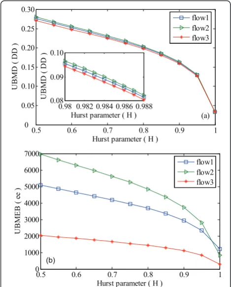
Figure 10 shows the impact of the Hurst parameterH on the upper bounds on multi-hops delay DD and multi-hops effective bandwidth ee in case of the self-similar microflows with the same Hurst parameters. We see a straightforward dependency: the upper bound on DDandeeare smaller for larger Hurst parameter.
The DD values and theee values decrease with the increasing of theHvalues under an increasing rate. The impact of the Hurst parameter on the DD values and theee values increase with the increase of the standard deviationsi,k. For instance, if H= 0.75,R= 100, T= 1, d = 2 and N = 10, then the DD and ee value of the flows: A1(t), A2(t) and A3(t) is 215.9, 218.9 and 212.1, and 3.95, 5.26 and 1.55, and ifH = 0.95 and the same values of other parameters mentioned above, the DD value and theee value of the three flows are 129, 131 and 127, and 2.34, 2.82 and 0.83, respectively.
Now, we assume that the Hurst parameters of the self-similar microflows have different values. For example, if
H1,1= 0.90,H1,2= 0.80,H1,3= 0.75,H2,1= 0.85,H2,2= 0.60 andH3,1 = 0.70, andR= 100,T= 1,d= 2 andN= 10, then theDD value and theeevalue of the flows:A1 (t), A2(t) and A3(t) is 222, 226 and 218, and 3.76, 5.74 and 1.65, respectively.
Besides, calculation and analysis of the node QoS and the single-hop QoS, such as the upper bounds on buffer queue length/delay/effective bandwidth of a sensor node, and the single-hop de-lay/jitter/effective band-width, and the multi-hops delay jitter in the WSNs with self-similar traffic flows are done, and the results are similar.
In this special case with self-similar traffic flows, we can obtain the guaranteed QoS by regulating the ser-vice rate R and the latency T of sensor nodes, as we can do in the case 2. The difference is that we use the fractal leaky bucket regulators to regulate the arrival self-similar traffic flows. Obviously getting the Hurst parameter of the arrival self-similar traffic flow is a key in advance in the case. Then, we can obtain the guar-anteed QoS by regulating the average arrival rater and the burst tolerance b of self-similar traffic flows in the WSNs.
Remark10: Recently, many related studies on determi-nistic end-to-end de-lays have done. Lenzini et al. [7] computed the end-to-end delay based on the LUDB methodology, but the delay is the minimum among all the delay bounds and the LUDB methodology cannot be applied directly to non-nested tandems. Schmitt et al. [8] achieved the worst-case end-to-end delays under blind multiplexing in tandem networks, and they dealt with arrival and service curves by a decomposition and re-composition scheme. Unlike Schmitt’s method, Bouil-lard et al. [9] directly computed the worst-case end-to-end delay instead of looking first for an end-to-end-to-end-to-end ser-vice curve by a decomposition and re-composition scheme, and may obtain a tighter bounds and a cheap complexity. Koubaa et al. [17-19] proposed closed-form recurrent expressions for computing the worst-case end-to-end delays across any source-destination path in a cluster-tree WSN. In this article, the proposed network-calculus-based models are simpler for computing the upper bounds on buffer queue length/delay/effective bandwidth and multi-hops/single-hop delay/jitter/effec-tive bandwidth using virtual buffer sharing in the WSNs, and these models are suitable for various flows, including self-similar traffic flows.
In summary, based on the numerical results and ana-lysis, we have found that the parameters of the flow reg-ulators and the service curves in the sensor nodes play an important role in modelling on a guaranteed QoS model for the WSNs, and have obtained the following findings: (1) the upper bound on buffer queue length is smaller for larger service rate with high-values, and it is
0.5 0.6 0.7 0.8 0.9 1
0 0.05 0.10 0.15 0.20 0.25 0.30
Hurst parameter ( H )
UBM
D (
DD )
(a) flow1 flow2 flow3
0.98 0.982 0.984 0.986 0.988 0.08
0.09 0.10
Hurst parameter ( H )
UBM
D (
DD )
0.5 0.6 0.7 0.8 0.9 1
0 1000 2000 3000 4000 5000 6000 7000
Hurst parameter ( H )
UBM
E
B (
e
e )
(b)
flow1 flow2 flow3
Figure 10The upper bounds on multi-hops delay (UBMD)DD (in s) and multi-hops effective bandwidth (UBMEB)ee(in Kb): (a)DDas a function of the Hurst parameterHforR= 100,T= 1,d
= 2 andN= 10;(b)eeas a function of the Hurst parameterHforR
smaller for larger evolution time or larger Hurst para-meter, and it is smaller for smaller latency or smaller service rate with low-values; (2) the upper bound on (multi-hops/single-hop) delay/jitter is smaller for larger service rate or larger Hurst parameter, and it is smaller for smaller latency or smaller hops; (3) the upper bound on (multi-hops/single-hop) effective bandwidth is larger for larger service rate, and it is smaller for larger latency or larger hops or larger Hurst parameter. In order to obtain network performance optimization and the guar-anteed QoS of the WSNs, including low delay for track-ing, we can reduce the upper bounds on (end-to-end) delay/jitter or increase the upper bounds on (end-to-end) effective bandwidth by designing the rational regu-lator parameters, including the average arrival rate and the burst tolerance, and the rational scheduler para-meters such as the service rate and the latency, of sen-sor nodes.
6. Conclusion
In this article, we have discussed the problem of the guaranteed QoS for flows. First, based on the arrival curve and the service curve in the network calculus, we have presented the system skeleton, involving the sensor node model on virtual buffer sharing, the flow source model and the two-layer scheduling model of sensor nodes and so on. Second, with the system skele-ton, we have not only drawn the node QoS model, such as the upper bounds on buffer queue length/ delay/effective bandwidth, but also drawn the single-hop/multi-hops QoS model, such as the upper bounds on single-hop/multi-hops delay/jitter/effective band-width. Finally, we have shown the practicability and the simplicity of the model and our approach using example results in the article. We can optimize net-work performances by designing reasonable regulators and schedulers of the WSNs nodes. A network calcu-lus approach is as a trade-off between complexity and accuracy. It is general, simple and practicable for pro-visioning the guaranteed QoS in the WSNs and other wireless networks with some characteristics of the dis-tribution and the multi-hops.
Ongoing and future works include: (1) implementing the algorithmic build upon the proposed network-calcu-lus-based model to ensure polynomial time complexity, for example, the computational complexity of node QoS algorithmic is O(cn), wherec is the number of micro-flows,nis the number of flows, and the computational complexity of buffer queue length algorithmic is O (c2n2), and the computational complexity of multi-hops/ single-hop QoS algorithmic is O(cnN), where Nis the number of hops; (2) investigating statistical sensor net-work calculus in order to capture the stochastic and dynamic behaviors of the WSNs.
Acknowledgements
This research was supported in part by the grant from the National Natural Science Foundation of China (60973129, 60903058 and 60903168), the China Postdoctoral Science Foundation funded project (200902324), the
Specialized Research Fund for the Doctoral Program of Higher Education (200805331109), the Scientific Research Fund of Hunan Provincial Education Department of China (10B062), the Program for Excellent Talents in Hunan Normal University (ET10902 and ET51102) and the Startup Project for Doctoral Research Supported by Scientific Research Fund of Hunan Normal University (110608). The material in this article was presented in part at First International Conference on Communications and Networking in China (ChinaCOM’06), Beijing, China, October 25-27, 2006, the International Workshop of Information Technology and Security (WITS’08), Shanghai, China, December 20-22, 2008, and the ISECS International Colloquium on Computing, Communication, Control, and Management (CCCM’08), Guangzhou, China, August 04-05, 2008. The authors would like to thank the reviewers for their valuable comments.
Author details
1College of Physics and Information Science, Hunan Normal University,
Changsha, Hunan 410081, China2College of Mathematics and Computer Science, Hunan Normal University, Changsha, Hunan 410081, China3Institute
of Information Science and Engineering, Central South University, Changsha, Hunan 410083, China
Competing interests
The authors declare that they have no competing interests.
Received: 21 February 2011 Accepted: 31 August 2011 Published: 31 August 2011
References
1. IF Akyildiz, T Melodia, KR Chowdhury, A survey on wireless multimedia sensor networks. Comput Netw.51(4), 921–960 (2007). doi:10.1016/j. comnet.2006.10.002
2. J Yick, B Mukherjee, D Ghosal, Wireless sensor network survey. Comput Netw.52(12), 2292–2330 (2008). doi:10.1016/j.comnet.2008.04.002 3. H Alemdar, C Ersoy, Wireless sensor networks for healthcare: a survey.
Comput Netw.54(15), 2688–2710 (2010). doi:10.1016/j.comnet.2010.05.003 4. R Kumar, M Wolenetz, B Agarwalla, J Shin, P Hutto, A Paul, U
Ramachandran, DFuse, a framework for distributed data fusion, in
Proceedings of 1st ACM Conference on Embedded Networked Sensor Systems (SenSys’03), (Los Angeles, CA, USA, November 2003), pp. 114–125 5. J-Y Le Boudec, P Thiran,Network Calculus, (Springer Verlag, 2004) 6. M Fidler, A survey of deterministic and stochastic service curve models in
the network calculus. IEEE Commun Surveys Tutor.12(1), 59–86 (2010) 7. L Lenzini, E Mingozzi, G Stea, End-to-end delay bounds in FIFO-multiplexing
tandems, inProceedings of the 2nd International Conference on Performance Evaluation Methodologies and Tools (VALUETOOLS’07), (Nantes, France, October 2007)
8. JB Schmitt, FA Zdarsky, M Fidler, Delay bounds under arbitrary multiplexing: when network calculus leaves you in the lurch ...., inProceedings of 27th IEEE International Conference on Computer Communications (INFOCOM’08), (Phoenix, AZ, USA, April 2008)
9. A Bouillard, L Jouhet, E Thierry, Tight performance bounds in the worst-case analysis of feed-forward networks, inProceedings of the 29th IEEE International Conference on Computer Communications (INFOCOM’10), (San Diego, CA, USA, March 2010), pp. 1316–1324
10. J Zhang, K Premaratne, PH Bauer, Resource allocation and congestion control in distributed sensor networks-a network calculus approach, in
Proceedings of Fifteenth International Symposium on Mathematical Theory of Networks and Systems (MTNS’02), (Notre Dame, Indiana, USA, August 2002) 11. JB Schmitt, U Roedig, Worst case dimensioning of wireless sensor networks
under uncertain topologies, inProceedings of the 1st workshop on Resource Allocation in Wireless Networks (RAWNET’05), (Washington, DC, USA, April 2005)
13. JB Schmitt, FA Zdarsky, U Roedig, Sensor network calculus with multiple sinks, inProceedings of IFIP Networking Workshop on Performance Control in Wireless Sensor Networks (PWSN’06), (Coimbra, Portugal, May 2006), pp. 6–13 14. JB Schmitt, FA Zdarsky, L Thiele, A comprehensive worst-case calculus for
wireless sensor networks with in-network processing, inProceedings of the 28th IEEE International Real-Time Systems Symposium (RTSS’07), (Tucson, AZ, USA, December 2007), pp. 193–202
15. Y Cao, Y Xue, Y Cui, Network-calculus-based analysis of power management in video sensor networks, inProceedings of the IEEE Global Communications Conference (GLOBECOM’07), (Washington, DC, USA, November 2007), pp. 981–985
16. H She, Z Lu, A Jantsch, L-R Zheng, D Zhou, Deterministic worst-case performance analysis for wireless sensor networks, inProceedings of the International Wireless Communications and Mobile Computing Conference (IWCMC’08), (Crete Island, Greece, August 2008), pp. 1081–1086 17. A Koubaa, M Alves, E Tovar, Modeling and worst-case dimensioning of
cluster-tree wireless sensor networks, inProceedings of the 27th IEEE International Real-Time Systems Symposium (RTSS’06), (Rio de Janeiro, Brazil, December 2006), pp. 412–421
18. A Koubaa, M Alves, E Tovar, Modeling and worst-case dimensioning of cluster-tree wireless sensor networks: proofs and computation details, (Technical Report, TR-060601, CISTER-ISEP Research Unit, Porto, Portugal, 2006)
19. P Jurcik, R Severino, A Koubaa, M Alves, E Tovar, Dimensioning and worst-case analysis of cluster-tree sensor networks. ACM Trans Sensor Netw.7(2), 14 (2010)
20. L Zhang, Z Chen, X Deng, G Huang, Y Liu, A scalable framework for QoS guarantees, inProceedings of First International Conference on
Communications and Networking in China (ChinaCom’06), (Beijing, China, October 2006)
21. L Zhang, Bounds on end-to-end delay jitter with self-similar input traffic an ad hoc wireless network, inProceedings of 2008 ISECS International Colloquium on Computing, Communication, Control, and Management (CCCM’08), (Guangzhou, China, August 2008), pp. 538–541 22. L Zhang, S Liu, H Xu, End-to-end delay in wireless sensor network by
network calculus, inProceedings of 2008 International Workshop on Information Technology and Security (WIST’08), (Shanghai, China, December 2008), pp. 179–183
23. H Qi, Z Chen, L Zhang, Towards end-to-end delay on WMNs based on statistical network calculus, inProceedings of the 9th International Conference for Young Computer Scientists (ICYCS’08), (Zhang Jia Jie, Hunan, China, November 2008), pp. 493–497
24. R-R Boorstyn, A Burchard, J Liebeherr, C Oottamakorn, Statistical service assurances for traffic scheduling algorithms. IEEE J Sel Areas Commun. 18(12), 2651–2662 (2002)
25. M Fidler, V Sander, A parameter based admission control for differentiated services networks. Comput Netw.44(4), 463–447 (2004). doi:10.1016/j. comnet.2003.12.004
26. G Procissi, A Garg, M Gerla, MY Sanadidi, Token bucket characterization of long-range dependent traffic. Comput Commun.25(11), 1009–1017 (2002). doi:10.1016/S0140-3664(02)00015-4
doi:10.1186/1687-1499-2011-82
Cite this article as:Zhanget al.:Modelling the guaranteed QoS for wireless sensor networks: a network calculus approach.EURASIP Journal on Wireless Communications and Networking20112011:82.
Submit your manuscript to a
journal and benefi t from:
7Convenient online submission
7 Rigorous peer review
7Immediate publication on acceptance
7 Open access: articles freely available online
7High visibility within the fi eld
7 Retaining the copyright to your article