R E S E A R C H
Open Access
Global existence of solutions for
interval-valued integro-differential equations
under generalized
H
-differentiability
Vinh An Truong
1, Van Hoa Ngo
2*and Dinh Phu Nguyen
3*Correspondence: [email protected] 2Division of Applied Mathematics, Ton Duc Thang University, Nguyen Huu Tho Street, District 7, Ho Chi Minh City, Vietnam
Full list of author information is available at the end of the article
Abstract
In this study, we consider the interval-valued integro-differential equations (IIDEs) under generalizedH-differentiability
DgHX(t) =F
(
t,X(t))
+ tt0
G
(
t,s,X(s))
ds, X(t0) =X0∈KC(R).The global existence of solutions for interval-valued integro-differential equations with initial conditions under generalizedH-differentiability is studied. Theorems for global existence of solutions are given and proved on [t0,∞). Some examples are given to illustrate these results.
MSC: 34K05; 34K30; 47G20
Keywords: interval-valued differential equations; interval-valued integro-differential equations; generalized Hukuhara derivative
1 Introduction
The set-valued differential and integral equations are an important part of the theory of set-valued analysis, and they play an important role in the theory and application of con-trol theory; and they were first studied in by De Blasi and Iervolino []. Recently, set-valued differential equations have been studied by many scientists due to their appli-cations in many areas. For the basic theory on set-valued differential and integral equa-tions, the readers can be referred to the following books and papers [–] and references therein. Integro-differential equations are encountered in many areas of science, where it is necessary to take into account aftereffect or delay (for example, in control theory, biology, ecology, medicine,etc.[–]). Especially, one always describes a model which possesses hereditary properties by integro-differential equations in practice.
The interval-valued analysis and interval differential equations (IDEs) are the special cases of the set-valued analysis and set-valued differential equations, respectively. In many situations, when modeling real-world phenomena, information about the behavior of a dy-namic system is uncertain and one has to consider these uncertainties to gain better mean-ing of full models. Interval-valued differential equation is a natural way to model dynamic systems subject to uncertainties. Recently, many works have been done by several authors in the theory of interval-valued differential equations (see,e.g., [–]). There are several
approaches to the study of interval differential equations. One popular approach is based onH-differentiability. The approach based onH-derivative has the disadvantage that it leads to solutions which have an increasing length of their support. Recently, Stefanini and Bede [] solved the above mentioned approach under strongly generalized differen-tiability of interval-valued functions. In this case, the derivative exists and the solution of an interval-valued differential equation may have decreasing length of the support, but the uniqueness is lost. The paper of Stefanini and Bede was the starting point for the topic of interval-valued differential equations (see [, ]) and later also for fuzzy differential equations. Also, a very important generalization and development related to the subject of the present paper is in the field of fuzzy sets,i.e., fuzzy calculus and fuzzy differential equations under the generalized Hukuhara derivative. Recently, several works,e.g., [, , , –], have been done on set-valued differential equations, fuzzy differential equa-tions and random fuzzy differential equaequa-tions.
In [, , ] the authors presented interval-valued differential equations under gener-alized Hukuhara differentiability which were given the following form:
X(t) =Ft,X(t), X(t) =X∈KC(R),t∈[t,T], (.)
wheredenotes two kinds of derivatives, namely the classical Hukuhara derivative and the second type Hukuhara derivative (generalized Hukuhara differentiability). The existence and uniqueness of a Cauchy problem is then obtained under an assumption that the coef-ficients satisfy a condition with the Lipschitz constant (see []). The proof is based on the application of the Banach fixed point theorem. In [], under the generalized Lipschitz condition, Malinowski obtained the existence and uniqueness of solutions to both kinds of IDEs.
In this paper, we study two kinds of solutions to IIDEs. The different types of solutions to IIDEs are generated by the usage of two different concepts of interval-valued derivative. This direction of research is motivated by the results of Stefanini and Bede [], Mali-nowski [, ] concerning deterministic IDEs with generalized interval-valued deriva-tive.
This paper is organized as follows. In Section , we recall some basic concepts and no-tations about interval analysis and interval-valued differential equations. In Section , we present the global existence of solutions to the interval-valued integro-differential equa-tions under two kinds of the Hukuhara derivative. Finally, we give some examples for IIDEs in Section .
2 Preliminaries
LetKC(Rn) be the space of nonempty compact and convex sets ofRn. The set of real
inter-vals will be denoted byKC(R). The addition and scalar multiplication inKC(R), we define
as usual,i.e., forA,B∈KC(R),A= [a–,a+],B= [b–,b+], wherea–≤a+,b–≤b+, andλ≥,
then we have
A+B=a–+b–,a++b+, λA=λa–,λa+ –λA=λa+,λa–.
Furthermore, let A∈KC(R), λ,λ,λ,λ∈R andλ,λ≥, then we have λ(λA) =
HinKC(R) is defined as follows:
H(A,B) =maxa––b–,a+–b+ . (.)
We notice that (KC(R),H) is a complete, separable and locally compact metric space. We
define the magnitude and the length ofA∈KC(R) by
HA,{}=A=maxa–,a+ , len(A) =a+–a–,
respectively, where{}is the zero element ofKC(R), which is regarded as one point. The
Hausdorff metric (.) satisfies the following properties:
H(A+C,B+C) =H(A,B) and H(A,B) =H(B,A),
H(A+B,C+D)≤H(A,C) +H(B,D),
H(λA,λB) =|λ|H(A,B)
for allA,B,C,D∈KC(R) andλ∈R. LetA,B∈KC(R). If there exists an intervalC∈KC(R)
such thatA=B+C, then we callCthe Hukuhara difference ofAandB. We denote the intervalC byAB. Note thatAB=A+ (–)B. It is known thatABexists in the caselen(A)≥len(B). Besides that, we can see [, , , ] the following properties for A,B,C,D∈KC(R):
- IfAB,ACexist, thenH(AB,AC) =H(B,C); - IfAB,CDexist, thenH(AB,CD) =H(A+D,B+C);
- IfAB,A(B+C)exist, then there exist(AB)Cand(AB)C=A(B+C); - IfAB,AC,CBexist, then there exist(AB)(AC)and
(AB)(AC) =CB.
Definition .[] We say that the interval-valued mappingX: [a,b]⊂R+→KC(R) is
continuous at the pointt∈[a,b] if for every> there existsδ=δ(t,) > such that, for alls∈[a,b] such that|t–s|<δ, one hasH(X(t),X(s))≤.
The strongly generalized differentiability was introduced in [] and studied in [, –].
Definition . LetX: [a,b]→KC(R) andt∈[a,b]. We say thatXis strongly generalized
differentiable attif there existsDgHX(t)∈KC(R) such that
(i) for allh> sufficiently small,∃X(t+h)X(t),∃X(t)X(t–h)and the limits
lim
hH
X(t+h)X(t)
h ,D
g HX(t)
= , lim
hH
X(t)X(t–h)
h ,D
g HX(t)
= ,
or
(ii) for allh> sufficiently small,∃X(t)X(t+h),∃X(t–h)X(t)and the limits
lim
hH
X(t)X(t+h) –h ,D
g HX(t)
= , lim
hH
X(t–h)X(t) –h ,D
g HX(t)
= ,
(iii) for allh> sufficiently small,∃X(t+h)X(t),∃X(t–h)X(t)and the limits
(hat denominators meansh). In this definition, case (i) ((i)-differentiability for short) cor-responds to the classicalH-derivative, so this differentiability concept is a generalization of the Hukuhara derivative. In [], Stefanini and Bede considered four cases for the deriva-tive. In this paper, we consider only the two first items of Definition .. In other cases, the derivative is trivial because it is reduced to a crisp element.
Remark .[, ] If for intervalsX,Y,Z∈KC(R) there exist Hukuhara differencesX
Y,XZ, thenH(XY,{}) =H(X,Y) andH(XY,XZ) =H(Y,Z).
LetX,Y: [a,b]→KC(R). We have (see []) some properties ofDgHas follows: (i) IfXis (i)-differentiable, then it is continuous.
(ii) IfX,Yare (i)-differentiable andλ∈R, thenDgH(X+Y)(t) =DgHX(t) +DgHY(t),
DgH(λX)(t) =λDgHX(t).
(iii) LetXbe (i)-differentiable and assume thatDgHXis integrable over[a,b]. Then we haveX(t) =X(a) +atDgHX(s)ds.
(iv) IfXis (i)-differentiable on[a,b], then the real functiont→len(X(t))is nondecreasing on[a,b].
(v) LetXbe (ii)-differentiable and assume thatDgHXis integrable over[a,b]. Then we haveX(a) =X(t) + (–)atDgHX(s)ds.
(vi) IfXis (ii)-differentiable on[a,b], then the real functiont→len(X(t))is nonincreasing on[a,b].
Corollary .(see,e.g., [, ]) Let X: [t,T]→KC(R)be given.Denote X(t) = [X–(t),
X+(t)]for t∈[t,T],where X–,X+: [t,T]→R.
(i) If the mappingXis(i)-differentiable(i.e.,classical Hukuhara differentiability)at
t∈[t,T],then the real-valued functionsX–,X+are differentiable attand
DgHX(t) = [(X–)(t), (X+)(t)].
(ii) If the mappingXis(ii)-differentiable att∈[t,T],then the real-valued functionsX–,
X+are differentiable attandDg
HX(t) = [(X+)(t), (X–)(t)].
Lemma .(see [, , ]) The interval-valued differential equation DgHX(t) =F(t,X(t)), X(t) =X∈KC(R),where F: [t,T]×KC(R)→KC(R)is supposed to be continuous,is
equivalent to one of the integral equations
X(t) =X+
t
t
or
X=X(t) + (–)
t
a
Fs,X(s)ds, ∀t∈[t,T]
on the interval [t,T]∈R,under the strong differentiability condition, (i)or(ii),
respec-tively.We notice that the equivalence between two equations in this lemma means that any solution is a solution for the other one.
We consider the Cauchy problem for IIDEs under the form
DgHX(t) =Ft,X(t)+
t
t
Kt,s,X(s)ds, X(t) =X (.)
for allt∈[t,T], whereF:I= [t,T]×KC(R)→KC(R) andK:D×KC(R)→KC(R) are
continuous interval-valued mappings onI, withD={(t,s)∈I×I:t≤s≤t<T}.
Definition . A mappingX: [t,T]→KC(R) is called a solution to problem (.) onI
if and only ifXis a continuous mapping onIand it satisfies one of the following interval-valued integral equations:
(S) X(t) =X+ (
t
tF(s,X(s))ds+ t
t s
tK(s,u,X(u))du ds),t∈I, ifXis (i)-differentiable or (iii)-differentiable.
(S) X(t) =X(–)(
t
tF(s,X(s))ds+ t
t s
tK(s,u,X(u))du ds),t∈I, ifXis (ii)-differentiable or (iv)-differentiable.
Definition . Let X : [t,T]→ KC(R) be an interval-valued function which is
(i)-differentiable. If Xand its derivative satisfy problem (.), we say Xis a (i)-solution of problem (.).
Definition . Let X: [t,T]→KC(R) be an interval-valued function which is
(ii)-differentiable. IfXand its derivative satisfy problem (.), we sayXis a (ii)-solution of problem (.).
Definition . A solutionX: [t,T]→KC(R) is unique ifsupt∈[t,T]H(X(t),Y(t)) = for
any mappingY: [t,T]→KC(R) that is a solution to (.) on [t,T].
Theorem .(see []) Let F:I= [t,T]×KC(R)→KC(R)and K:D×KC(R)→KC(R)
be continuous interval-valued mappings on I.Suppose that there exists L> such that
maxHF(t,X),F(t,X)
,HK(t,s,X),K(t,s,X) ≤LH(X,X)
for all t,s∈I,X,X∈KC(R).Then there exists the only local solution X to IIDE(.)on
some intervals[t,T] (T≤T–t)for each case((i)-solution and(ii)-solution).
3 Main results
In this section of the paper, we consider again the following initial value problem for the interval-valued integro-differential equations (IIDEs) under the form
DgHX(t) =Ft,X(t)+
t
t
for all t∈J= [t,∞), whereF:J×KC(R)→KC(R) andK:D×KC(R)→KC(R) are
continuous interval-valued mappings onJ, withD={(t,s)∈J×J:t≤s≤t<∞}.
Theorem . Assume that
(i) F(t,X),G(t,s,X)are locally Lipschitzian for allt,s∈J,X∈KC(R);
(ii) f∈C[J×[,∞), [,∞)]andk∈C[D×[,∞), [,∞)]are nondecreasing inx≥, and the maximal solutionr(t,t,x)of the scalar integro-differential equation
x(t) =ft,x(t)+
t
t
kt,s,x(s)ds, x(t) =x≥, (.)
exists throughoutJ;
(iii) H(F(t,X),{})≤f(t,H(X,{})),H(K(t,s,X),{})≤k(t,s,H(X,{}))for allt,s∈J,
X∈KC(R);
(iv) H(X(t,t,X),{})≤r(t,t,x),H(X,{})≤x.
Then the largest interval of the existence of any solution X(t,t,X)of(.)for each case
((i)-solution and(ii)-solution)such that H(X,{})≤xis J.In addition,if r(t,t,x)is
bounded on J,thenlimt→∞X(t,t,X)exists in(KC(R),H).
Proof Since the way of the proof is similar for both cases ((i)-solution and (ii)-solution), we only prove case (i)-differentiability. By hypothesis (i), there exists aT>tsuch that the
unique (i)-solution of problem (.) exists on [t,T]. Let
S=X(t)|X(t) is defined on [t,αX] and is the (i)-solution to (.) .
Then S=∅. Takingα=sup{αX|X(t)∈S}, clearly, there exists a unique (i)-solution of
problem (.) which is defined on [t,α) withH(X,{})≤x. Next, we shall prove that
α=∞. We supposeα<∞and define
m(t) =HXt,t,X,{}
, t≤t<α.
Using assumptions (ii) and (iii), we have
D+m(t) =lim inf
t→+
H(X(t+h,t,X),{}) –H(X(t,t,X),{})
h
≤lim inf
h→+
H(X(t+h,t,X),X(t,t,X))
h
=lim inf
h→+
H(X(t+h,t,X)X(t,t,X),{})
h
=HDgHX(t),{}=H
Ft,X(t)+
t
t
Kt,s,X(s)ds,{}
≤HFt,X(t),{}+
t
t
HKt,s,X(s),{}ds
≤ft,m(t)+
t
t
andm(t) =H(X,{})≤x. Further, by assumption (iv), it follows thatm(t)≤r(t,t,x),
By the assumption (i) again, it follows thatX(t) can be extended beyondα, which con-tradicts our assumption. So, any (i)-solution of problem (.) exists onJ= [t,∞), and so
α=∞.
Example . Consider the IIDE
DgHX(t) =a(t)X(t) +
t
t
b(s)X(s)ds, X(t) =X, (.)
where we assume that a(t),b(t) : R+ → R+ are continuous functions. We see that
F(t,X(t)) =a(t)X(t) andK(t,s,X(t)) =b(t)X(t) are locally Lipschitzian. If we letf(t,x(t)) =
Theorem . Assume that
(iii) The maximal solutionr(t) =r(t,t,x)of the scalar integro-differential equation
x(t) =ft,x(t)+
onJX. We shall first show thatSis nonempty. Indeed, by assumption (i), there exists a
(i)-solutionX(t) of problem (.) defined onJX= [t,cX). LetX(t) =X(t,t,X) be any
(i)-solution of (.) existing onJX. Definek(t) =V(t,X(t)) so thatk(t) =V(t,X)≤x. Now,
for smallh> and using assumption (ii), we consider
using the Lipschitz condition in assumption (ii). Thus
Therefore, we have the scalar integro-differential inequality
D+k(t)≤ft,k(t)+
t
t
kt,s,x(s)ds, k(t)≤x.
According to Proposition . in [], we get the estimate
k(t)≤r(t,t,x), t∈IX.
It follows that
Vt,X(t)≤r(t,t,x), t∈IX, (.)
We have, for allt,t∈JZwitht≤t,
The assumption of local existence implies that there exists a (i)-solutionX(t) on [cZ,cZ+
(iii) The maximal solutionr(t) =r(t,t,x)of the scalar integro-differential equation
x(t) =ft,x(t)+
t
t
kt,s,x(s)ds, x(t) =x≥, (.)
exists onJand is positive wheneverx> .
Then,for every X∈KC(R)such that V(t,X)≤x,problem(.)has a(ii)-solution X(t)
on[t,∞),which satisfies the estimate
Vt,X(t)≤r(t,t,x), t≥t. (.)
Proof One can obtain this result easily by using the methods as in the proof of Theo-rem ..
4 Some examples
In this section, we present some examples being simple illustrations of the theory of IIDEs. We will consider IIDEs (.) with (i) and (ii) derivatives, respectively. For convenience, from now on, we denote the solution of IIDE (.) with (i) derivative byXand the solution
with (ii) derivative byX.
Let us start the illustrations by considering the following interval-valued integro-differential equation:
DgHX(t) =F(t) +
t
t
k(t,s)X(s)ds, X(t) =X=
X–,X+,t∈[t,T], (.)
whereF: [t,T]→KC(R) is an interval-valued function (i.e.,F(t) = [F–(t),F+(t)]),k(t,s)
is a real known function, andX∈KC(R). In equation (.), we shall solve it by two types
of the Hukuhara derivative, which are defined in Definition .. Consequently, based on the type of differentiability, we have the following two cases.
Case : Suppose thatX(t) in equation (.) is (i)-differentiable. By using Corollary ., then we getDgHX(t) = [(X–(t)), (X+(t))]. Hence, we have the following:
⎧ ⎨ ⎩
(X–(t))=F–(t) +t
tk(t,s)X(s)ds,
(X+(t))=F+(t) +t
tk(t,s)X(s)ds,
(.)
where
k(t,s)X(s)ds=
⎧ ⎨ ⎩
k(t,s)X–(t), k(t,s)≥, k(t,s)X+(t), k(t,s) <
and
k(t,s)X(s)ds=
⎧ ⎨ ⎩
k(t,s)X+(t), k(t,s)≥,
From (.), we have
Case : Suppose thatX(t) in (.) is (ii)-differentiable, then we proceed as in Case . Hence (.) can be rewritten in the sense of (ii)-differentiability as follows:
⎧
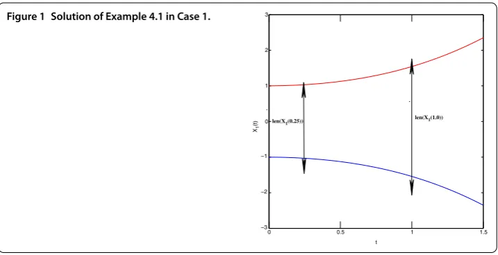
Example . Let us consider the following IIDE:
DgHX(t) =
], and this solution is shown in
Figure .
Case . From (.), we get
⎧ ⎪ ⎪ ⎪ ⎪ ⎪ ⎨ ⎪ ⎪ ⎪ ⎪ ⎪ ⎩
(X+(t))=t
X–(s)ds,
(X–(t))=t
X +(s)ds,
X–() = –,
x+() = .
(.)
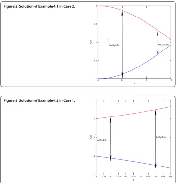
By solving IDEs (.), we obtainX(t) = [–cos(t),cos(t)], and this solution is shown in
Figure .
Example . Let us consider the following IIDE:
DgHX(t) = [–, ] +
t
X(s)ds, X() =X= [–, ],t∈[, .]. (.)
Case . We obtainX(t) = [–et, et], and this solution is shown in Figure .
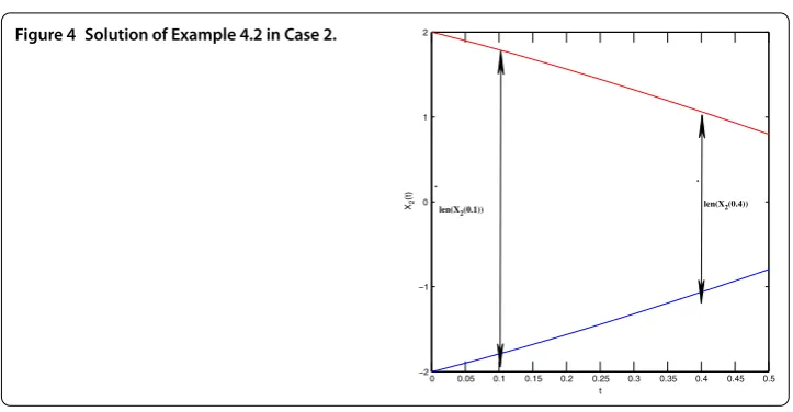
Case . We obtain X(t) = [–cos(t) + sin(t), cos(t) – sin(t)], and this solution is
shown in Figure .
Figure 2 Solution of Example 4.1 in Case 2.
Figure 4 Solution of Example 4.2 in Case 2.
As we see in figures, the first type and second type Hukuhara differentiable interval-valued solutionsXbehave in various ways,i.e., one can say thatlen(X(t)) in examples is
nondecreasing in time (see Figures and ) andlen(X(t)) in examples is nonincreasing in
time (see Figures and ).
5 Conclusions and further work
From Example . to Example ., we notice that the solutions under the classical Hukuhara derivative ((i)-differentiable) have increasing length of their values. Indeed, we can see this in Figures and . However, if we consider the second type Hukuhara deriva-tive ((ii)-differentiable), the length of solutions changes. Under the second type Hukuhara derivative, differentiable solutions have nonincreasing length of its values (see Figures and ). In [, ], authors introduced and studied new generalized differentiability con-cepts for interval-valued functions. Our point is that the generalization of this concept can be of great help in the dynamic study of interval-valued differential equations and interval-valued integro-differential equations.
Competing interests
The authors declare that they have no competing interests.
Authors’ contributions
All authors read and approved the final version of the manuscript.
Author details
1Faculty of Foundation Sciences, University of Technical Education, Ho Chi Minh City, Vietnam.2Division of Applied Mathematics, Ton Duc Thang University, Nguyen Huu Tho Street, District 7, Ho Chi Minh City, Vietnam.3Faculty of Mathematics and Computer Science, University of Science, VNU, Ho Chi Minh City, Vietnam.
Acknowledgements
The authors would like to express their gratitude to the anonymous referees for their helpful comments and suggestions, which have greatly improved the paper. The first named author would like to thank the University of Technical Education, Ho Chi Minh City, Vietnam.
Received: 10 January 2013 Accepted: 8 July 2013 Published: 22 July 2013 References
1. De Blasi, FS, Iervolino, F: Equazioni differenziali con soluzioni a valore compatto convesso. Boll. Unione Mat. Ital.4(2), 194-501 (1969)
2. Agarwal, RP, O’Regan, D: Existence for set differential equations via multivalued operator equations. Differ. Equ. Appl.
5, 1-5 (2007)
4. Agarwal, RP, O’Regan, D, Lakshmikantham, V: A stacking theorem approach for fuzzy differential equations. Nonlinear Anal. TMA55(3), 299-312 (2003)
5. Devi, JV: Generalized monotone iterative technique for set differential equations involving causal operators with memory. Int. J. Adv. Eng. Sci. Appl. Math. (2011). doi:10.1007/s12572-011-0031-1
6. Ngo, VH, Nguyen, DP: On maximal and minimal solutions for set-valued differential equations with feedback control. Abstr. Appl. Anal. (2012). doi:10.1155/2012/816218
7. Kaleva, O: Fuzzy differential equations. Fuzzy Sets Syst.24, 301-317 (1987)
8. Lakshmikantham, V, Bhaskar, TG Devi, JV: Theory of Set Differential Equations in Metric Spaces. Cambridge Scientific Publisher, Cambridge (2006)
9. Puri, M, Ralescu, D: Differentials of fuzzy functions. J. Math. Anal. Appl.91, 552-558 (1983)
10. Lakshmikantham, V, Mohapatra, R: Theory of Fuzzy Differential Equations and Inclusions. Taylor & Francis, London (2003)
11. De Blasi, FS, Lakshmikantham, V, Bhaskar, TG: An existence theorem for set differential inclusions in a semilinear metric space. Control Cybern.36(3), 571-582 (2007)
12. Song, S, Wu, C: Existence and uniqueness of solutions to Cauchy problem of fuzzy differential equations. Fuzzy Sets Syst.110, 55-67 (2000)
13. Bhaskar, TG, Lakshmikantham, V: Set differential equations and flow invariance. J. Appl. Anal.82(2), 357-368 (2003) 14. Hale, JK: Theory of Functional Differential Equations. Springer, New York (1977)
15. Kolmanovskii, VB, Myshkis, A: Applied Theory of Functional Differential Equations. Kluwer Academic, Dordrecht (1992) 16. Park, JY, Jeong, JU: On existence and uniqueness of solutions of fuzzy integro-differential equations. Indian J. Pure
Appl. Math.34(10), 1503-1512 (2003)
17. Stefanini, L, Bede, B: Generalized Hukuhara differentiability of interval-valued functions and interval differential equations. Nonlinear Anal. TMA71, 1311-1328 (2009). doi:10.1016/j.na.2008.12.005
18. Chalco-Cano, Y, Rufián-Lizana, A, Román-Flores, H, Jiménez-Gamero, MD: Calculus for interval-valued functions using generalized Hukuhara derivative and applications. Fuzzy Sets Syst. (2012). doi:10.1016/j.fss.2012.12.004
19. Malinowski, MT: Interval Cauchy problem with a second type Hukuhara derivative. Inf. Sci.213, 94-105 (2012). doi:10.1016/j.ins.2012.05.022
20. Malinowski, MT: Interval differential equations with a second type Hukuhara derivative. Appl. Math. Lett.24, 2118-2123 (2011)
21. Allahviranloo, T, Hajighasemi, S, Khezerloo, M, Khorasany, M, Salahshour, S: Existence and uniqueness of solutions of fuzzy Volterra integro-differential equations. In: IPMU. CCIS, vol. 81, pp. 491-500 (2010)
22. Allahviranloo, T, Amirteimoori, A, Khezerloo, M, Khezerloo, S: A new method for solving fuzzy Volterra integro-differential equations. Aust. J. Basic Appl. Sci.5(4), 154-164 (2011)
23. Allahviranloo, T, Salahshour, S, Abbasbandy, S: Solving fuzzy fractional differential equations by fuzzy Laplace transforms. Commun. Nonlinear Sci. Numer. Simul.17(3), 1372-1381 (2012). doi:10.1016/j.cnsns.2011.07.005 24. Allahviranloo, T, Abbasbandy, S, Sedaghatfar, O, Darabi, P: A new method for solving fuzzy integro-differential
equation under generalized differentiability. Neural Comput. Appl.21(1), 191-196 (2012). doi:10.1007/s00521-011-0759-3
25. Allahviranloo, T, Ghanbari, M, Haghi, E, Hosseinzadeh, A, Nouraei, R: A note on ’Fuzzy linear systems’. Fuzzy Sets Syst.
177, 87-92 (2011)
26. Alikhani, R, Bahrami, F, Jabbari, A: Existence of global solutions to nonlinear fuzzy Volterra integro-differential equations. Nonlinear Anal. TMA75(4), 1810-1821 (2012)
27. Bede, B, Gal, SG: Generalizations of the differentiability of fuzzy-number-valued functions with applications to fuzzy differential equations. Fuzzy Sets Syst.151, 581-599 (2005)
28. Bede, B, Rudas, IJ, Bencsik, AL: First order linear fuzzy differential equations under generalized differentiability. Inf. Sci.
177, 1648-1662 (2007)
29. Bede, B, Stefanini, L: Generalized differentiability of fuzzy-valued functions. Fuzzy Sets Syst. (2012). doi:10.1016/j.fss.2012.10.003
30. Bede, B: A note on ’Two-point boundary value problems associated with non-linear fuzzy differential equations’. Fuzzy Sets Syst.157(7), 986-989 (2006)
31. Chalco-Cano, Y, Román-Flores, H: On new solutions of fuzzy differential equations. Chaos Solitons Fractals38, 112-119 (2008)
32. Lakshmikantham, V, Tolstonogov, AA: Existence and interrelation between set and fuzzy differential equations. Nonlinear Anal. TMA55(3), 255-268 (2003)
33. Stefanini, L, Sorini, L, Guerra, ML: Parametric representation of fuzzy numbers and application to fuzzy calculus. Fuzzy Sets Syst.157, 2423-2455 (2006)
34. Nguyen, DP, Ngo, VH, Ho, V: On comparisons of set solutions for fuzzy control integro-differential systems. J. Adv. Res. Appl. Math.4(1), 84-101 (2012). doi:10.5373/jaram
35. Zhang, D, Feng, W, Zhao, Y, Qiu, J: Global existence of solutions for fuzzy second-order differential equations under generalizedH-differentiability. Comput. Math. Appl.60, 1548-1556 (2010)
36. Malinowski, MT: Random fuzzy differential equations under generalized Lipschitz condition. Nonlinear Anal., Real World Appl.13(2), 860-881 (2012)
37. Malinowski, MT: Existence theorems for solutions to random fuzzy differential equations. Nonlinear Anal., Theory Methods Appl.73(6), 1515-1532 (2010)
38. Malinowski, MT: On random fuzzy differential equations. Fuzzy Sets Syst.160(21), 3152-3165 (2009) 39. Mizukoshi, MT, Barros, LC, Chalco-Cano, Y, Román-Flores, H, Bassanezi, RC: Fuzzy differential equations and the
extension principle. Inf. Sci.177, 3627-3635 (2007)
40. Malinowski, MT: On set differential equations in Banach spaces - a second type Hukuhara differentiability approach. Appl. Math. Comput.219(1), 289-305 (2012)
41. Malinowski, MT: Second type Hukuhara differentiable solutions to the delay set-valued differential equations. Appl. Math. Comput.218(1), 9427-9437 (2012)
doi:10.1186/1687-1847-2013-217