Development of an automatic procedure to estimate the reflection height of
tweek atmospherics
Hiroyo Ohya1, Kazuo Shiokawa2, and Yoshizumi Miyoshi2
1Graduate School of Engineering, Chiba University, 1-33 Yayoi-cho, Inage-ku, Chiba 263-8522, Japan 2Solar-Terrestrial Environment Laboratory, Nagoya University, Furo-cho, Chikusa-ku, Nagoya 464-8601, Japan
(Received February 15, 2008; Revised May 2, 2008; Accepted May 8, 2008; Online published September 8, 2008)
This paper presents an automated procedure to estimate apparent reflection heighth(from the cutoff frequency for the first waveguide mode, fc), horizontal propagation distanced, and propagation time Tg of tweek
atmo-spherics. Tweek data recorded at the Kagoshima Observatory (31.48◦N, 130.72◦E), Japan, were used to evaluate the procedure by comparing the results estimated by the automatic method to those read manually by an operator. The two types of results showed differences (automatic−manual) of+0.58 km,−9.9 Hz, and+3058.9 km for meanh, fc, andd, respectively. The difference inh(fc)was less than the resolution of the fast Fourier transform
used to obtain the tweek spectra. These comparisons indicate that the automatic estimation procedure of tweek parameters developed in this paper performs well and is a useful tool for studying long-term height variations of the ionosphericDand lower E regions using very low frequency (VLF) and extremely low frequency (ELF) records observed in Japan over the past 30 years.
Key words:Tweek atmospherics, reflection height,D-region ionosphere, low latitudes.
1.
Introduction
The nighttime D-region ionosphere at altitudes of 60– 90 km is produced from photoionization by geocoronal emissions as well as ionization by radiation belt particles at middle and low latitudes (e.g., Tohmatsu, 1990). Thus, measurements of the nighttime D-region at low latitudes can be used to monitor these effects, particularly those of radiation belt particles during geomagnetic storms.
Strong coupling between the D-region ionosphere and the neutral atmosphere makes D-region measurements dif-ficult. For example, the electron density of the D-region is too low to be measured by conventional ionosondes with frequencies of 1–30 MHz. The altitude of the D-region is too low for satellite measurements of electron density and too high for balloon measurements. Thus, sounding rocket experiments have been used to directly measure the D -region electron density profiles (e.g., Maeda, 1971). How-ever, sounding rockets can only be launched from limited locations and obtain limited frequencies. The recent devel-opment of medium frequency (MF) radar has enabled con-tinuous measurements of electron density in the D-region (e.g., Holdsworthet al., 2002), although drawbacks of MF radars include their need for rather large facilities as well as large amounts of electrical power. Standard radio-wave signals propagated from very low frequency/low frequency (VLF/LF) transmitters have also been used to measure the height variation of theD-region, based on phase and inten-sity modulations (e.g., Bickelet al., 1970; Thomas and Har-rison, 1970; Thomson, 1993). However, the region
avail-Copyright cThe Society of Geomagnetism and Earth, Planetary and Space Sci-ences (SGEPSS); The Seismological Society of Japan; The Volcanological Society of Japan; The Geodetic Society of Japan; The Japanese Society for Planetary Sci-ences; TERRAPUB.
able for electron density measurements by this method is restricted along the propagation path between the transmit-ter and the receiver.
Ohyaet al.(2003) proposed a technique to measure the
D-region height variations using VLF/extremely low fre-quency (ELF) tweek atmospherics (1.5–10.0 kHz) origi-nating from lightning discharges. Passive measurement of VLF/ELF tweeks is much easier and cheaper than measure-ment by active radars. Moreover, since the tweek atmo-spherics can always be detected, the technique is a power-ful tool for deriving the long-term variation of theD-region height. The technique is based on the fact that the first-order mode cut-off frequency of tweek atmospherics is a significant indicator of tweek reflection heights (equivalent electron densities) in theD-region ionosphere. Tweeks are reflected by the D- and lower E-region ionosphere at alti-tudes below 100 km where the electron density becomes 20–28 cm−3 (Shvets and Hayakawa, 1998; Ohya et al.,
2003) and propagate long distances (a few thousand kilo-meters) in the Earth-ionosphere waveguide (Outsu, 1960; Yamashita, 1978; Hayakawaet al., 1994, 1995; Shvets and Hayakawa, 1998). As for the polarization of the tweeks, the zero-order mode of tweeks is expected to be TM0
(trans-verse magnetic) mode (Wait, 1972), in agreement with the observations by Hayakawaet al.(1994). For the first-order mode, both TM and TE (transverse electric) modes were considered by Hayakawa et al.(1994) based on an inho-mogeneous and anisotropic ionosphere model. Yamashita (1978) showed by calculating attenuation coefficient and excitation factor of the waveguide near the cut-off frequen-cies that QTE (quasi-TE) mode plays a dominant role in the formation of tweeks. Ferencz (2004) presented a new theoretical model of waveguide and numerical solutions of
the model. Ferenczet al.(2007) recently reported by using VLF recordings on board the DEMETER satellite that spe-cific signals of fractional hop whistlers, “Spiky Whistler”, are excited by tweeks.
From the cut-off frequency of the first mode of tweeks, the apparent reflection heighth can be estimated. Lower (higher) h corresponds to increased (decreased) electron density in the D-region ionosphere. Thus, thehvalue ob-tained from tweeks is a useful parameter for investigating electron density variations in the nighttime D-region iono-sphere (e.g., Ohyaet al., 2003, 2006). The h denotes the height of the waveguide averaged over the propagation path (Hayakawaet al., 1994). Since a few hundred tweeks are received in 1 minute at night and the various propagation paths of those tweeks can be detected, the tweek method is a powerful tool for investigating the variations in the D -region height over a wide area. Moreover, it is possible to investigate the height variations during various geophysical time scales such as during magnetic storms and solar cycles. In Japan, tweek atmospherics have been observed at the Moshiri (44.37◦N, 142.27◦E) and Kagoshima (31.48◦N, 130.72◦E) observatories of the Solar-Terrestrial Envi-ronment Laboratory, Nagoya University, for more than 30 years. With this 30-year dataset, analysis of the long-term variations of the D-region and lower E-region iono-sphere is possible. However, for efficient analysis of a long-term dataset, a new method that can detect tweeks and es-timate the cut-off frequency automatically is essential. In this study, we developed such a method and verified it by comparing the parameters obtained by automatic and con-ventional manual methods.
2.
Automatic Method with a Spherical Waveguide
Model
2.1 Spherical waveguide model
The routine for automatic estimation of the ionosphere parameter was based on a homogeneous spherical Earth-ionosphere waveguide model (Davies, 1969). The horizon-tal phase velocityvp in the homogeneous spherical
Earth-ionosphere waveguide is approximated by
vp≈
c
1−h
a
1−
nλ
2h
2 (1)
wherecis the light velocity,h is the height of the waveg-uide, a is the Earth’s radius, λ is the wavelength in free space, and n is the order of mode. The denominator of Eq. (1) indicates real part of sine of the incident angle to calculate the horizontal group velocity. Equation (2) gives
has
h= nc
2fc
(2)
where fcis the cut-off frequency. We do not need to take
the number of reflections into account, although multiple reflections in the waveguide are geometrically described by image sources placed along vertical axis at the points, 0,
±2h,±4h,. . .when we assume a vertical dipole for
light-ning discharge on the ground (Wait, 1972). We estimate the
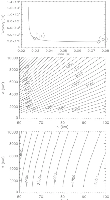
Fig. 1. (Top panel) frequency-time curve of an artificial tweek, (middle panel) dependence of the parameterhanddon the frequency of the tweek at the time of (a), and (bottom panel) dependence of the parameter
handdon the frequency of the tweek at the time of (b). In the middle and bottom panels, the contour lines with the numbers indicate the frequencyf (Hz) of the tweeks.
cut-off frequency for the first-order mode. The cut-off fre-quency (or cut-off wavelength) is determined by the height of the waveguide. The horizontal group velocityvgfor the
first-order mode is obtained from Eqs. (1) and (2) forn=1 as follows:
vg ≈
c2
vp
=
c
1−
fc f
2
1− c
2a fc
(3)
where f is the frequency of the waves. The propagation timeTgfor the first-order mode is obtained from Eq. (4):
Tg= d
=
d
1− c
2a fc
c
1−
fc f
2 (4)
whered is the horizontal propagation distance of tweeks. Consequently, the frequency-time dispersion relation of tweeks is rewritten as follows:
f = Tgfc
1− c
2a fc T2
g −
d c
2. (5)
In Eq. (5), unknown parameters are fc, d, and Tg. Here Tg is the time delay from the lightning to the observation
point for each frequency. For easier calculation of these unknown parameters, we transformed Eq. (5). We assumed that the unknown parameter Tg is the time from lightning
occurrence to the first point t0, wheret0 is the first time
the tweek is identified on the dynamic spectrum. Thus, we can uset0 =Tg,t1 =Tg +time step,t2 =Tg +time
step × 2, . . ., andtn = Tg +time step × N. Then, by
using the gradient-expansion algorithm, we fitted Eq. (5) to the dataset of (ti, fi) for i = 0,1,2, . . . ,N, which was determined from the dynamic spectrum, as described in Section 2.2.
Figure 1 shows dependence of the parameters h and d
on the frequency f. Top panel shows a typical frequency-time curve of an artificial tweek. Middle panel shows the dependence of thehanddon the f at the time of (a). The
x, andyaxes indicateh(km) andd (km), respectively, and the contour indicates f (Hz). The middle panel shows that
d is more sensitive to the frequency changes thanh at the time of the maximum curvature. The bottom panel shows the dependences at the time of (b) in the top panel. This
panel indicates thathbecomes more sensitive to f-changes at the tweek tail.
2.2 Automatic method
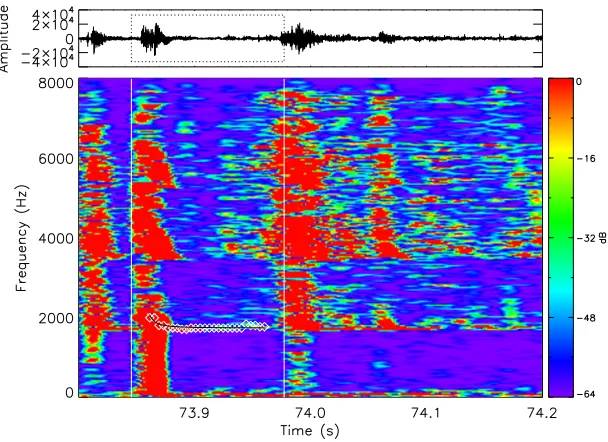
Figure 2 shows an example of tweek atmospherics ob-served at Kagoshima at 17:51 UT (02:51 LT) on 1 Novem-ber 2003. A tweek atmospheric was observed at 73.84– 73.95 s (17:51:13.84–17:51:13.97 UT), as indicated by the two white vertical lines illustrating the analyzed time inter-val. The frequencies decreased from 4–2 kHz to just below 2 kHz, showing a characteristic dispersion. The cut-off fre-quency of the first-order mode was found below 2 kHz, and the frequency below the cut-off frequency corresponded to the zero-order mode. By fitting a theoretical curve to these observed tweeks, the parametersh,d, andTg can be
esti-mated. We adopted the gradient-expansion algorithm to fit the theoretical function of Eq. (5) based on the homoge-neous spherical waveguide model.
At the Kagoshima and Moshiri observatories, the waveforms (an east-west magnetic component) of these VLF/ELF atmospherics in a wide frequency range (0– 10 kHz) have been recorded for 2 minutes of every hour (from minutes 50 to 52) since April 1976 onto analog tapes
and mini-disks. Because sampling for each entire hour
would produce massive amounts of VLF/ELF data, only the 2-min interval per hour has been recorded continuously for more than 30 years. These analog tweek waveforms were digitized into a hard disk with a 16-bit A/D converter with a 20-kHz sampling frequency. The automated procedure first picks up intense tweeks, which have amplitudes exceeding 80% of the maximum amplitude of the 2 minutes. By this method, the tweek level should vary among the 2-minute datasets. We cannot discuss the intensity variations of VLF data over the long term because the variations depend not only on the condition of the D-region and lower E-region but also on the observational system itself. On the other hand, the reflection-height variations of tweeks do not
pend on the observational system and are useful for investi-gating long-term change.
Next, the procedure searches the frequency fi of the maximum power of the spectrum at every sampling time
ti (50 μs) for time intervals from 30 ms before to 70 ms
after the time triggered by shifting the fast Fourier trans-form (FFT) window (25.6 ms) by one sampling timeti on the dynamic spectrum. The duration of tweeks is typically
∼50 ms. Considering that the longest tweeks last∼100 ms, we empirically set the time intervals of 100 ms to have enough fitting precision and to exclude the next (non-target) tweeks. The first time interval of 30 ms needs to obtain the higher-frequency part of the tweeks. The last time interval of 70 ms is long enough to obtain the data points of the tweek tail. Then, to remove background noise emissions and other tweeks embedded on the target tweek, the proce-dure selects the dataset (ti, fi) for one tweek automatically by checking the frequency difference between two succes-sive times,ti andti+1. However, if more than two tweeks
with comparable intensities overlap, the procedure cannot clearly distinguish them and fails to determine the param-eters. Such cases can be finally removed, since the fitting error (expressed as chi-squared below) becomes very large, and the estimated parameterd becomes unrealistic (either less than 1,000 km or more than 10,000 km) for such cases. For the least-square fitting, we adopted the fitting results when the mean difference between the data point fi and the fitted curve was less than 50 Hz, which is comparable to the FFT frequency resolution (40 Hz). The fitting results with large differences should thus be ruled out.
3.
Comparison to the Manual Method
3.1 Evaluation of the developed method using artificial tweeks
To see the difference between the automated and manual method, we first compared the frequency data points
de-termined by the automated and manual methods by using waveforms of artificial tweeks. We calculated the frequen-cies f of the artificial tweek using Eq. (5) and produced the waveformy(t)=sin(2πf t). The amplitude and initial
phase were assumed to be 1 and 0, respectively.
Figure 3 shows a frequency-time spectra of an artificial tweek with fc=1700 Hz andd =6000 km. White points
and diamonds indicate the data points determined by the au-tomatic procedure and by the manual method, respectively. The solid and dotted curves are the fitting curve by the au-tomatic procedure and the input frequency-time curve, re-spectively. The results of the estimation were fc=1659.18
±0.13 Hz andd =9408.16±0.50 km for the automated
method, and fc=1712.17±0.07 Hz andd =7125.96±
0.07 km for the manual method, respectively. This means that the automatic procedure can recognize correct peak of the tweek signals.
To investigate the fitting accuracy of the manual method, we generated 9 artificial tweeks that have a parameter com-bination of fc=1500, 2000 and 2500 Hz, andd =1000,
6000 and 10000 km. We estimated fcanddfor these
artifi-cial tweeks by the manual method and compared the fitting results with original input values. As the results, the aver-age fitting error of the fcwas+0.716%. The fitting error
of theddecreased for longerd, i.e., the average errors were
+35.494% ford =1000 km,+18.766% ford =6000 km,
and+0.292% ford=10000 km, respectively. This means that tweek signals with short duration of frequency-time dispersion are more difficult for estimatingd.
Next we checked whether the artificial tweeks could be picked up by the automatic procedure according to
our tweek selection alogorithm. All tweeks with
non-overlapped time intervals of more than 50 ms before and after the tweek signals could be picked up by the automatic procedure (100 of 100 tweeks). The automatic procedure did not pick up the tweeks for which other tweeks were
overlapped during time interval less than 50 ms before and after the target tweek, because of our tweek-selection crite-ria.
3.2 Comparison using observation data
We compared tweek parameters estimated by the auto-mated and manual methods with the spherical model, us-ing 77 tweeks recorded at Kagoshima at 17:50–17:52 UT (02:50–02:52 LT) on 1 November 2003. The automatic pro-cedure picked up 266 tweeks. For 93 of those 266 tweeks, the typical dispersion relation could not be found by vi-sual inspection in the manual method. For the remaining 173 tweeks, 96 had a large fitting error (>50 Hz). These large-error events were mainly caused by the overlapping of more than two tweeks on the dynamic spectrum, as will be discussed later. Thus, we used the other 77 tweeks for the comparison. For each tweek, we compared the auto-matic estimation results of h(fc)andd to those from the
manual method, in which an operator selects (ti, fi) based on visual inspection of the dynamic spectrum and calculates the parameters using Eq. (5).
Figure 2 shows an example of good fitting by the auto-matic method (the mean difference between the data point
fi and the fitted theoretical curve is 42.0 Hz). The tar-get tweek was observed at 73.84–73.95 s at frequencies of
∼2 kHz, as shown by the two white vertical lines indicating the analyzed time interval. The white points and the black line mark the peak frequencies of the tweek and the esti-mated frequency-time curve, respectively. In this case, the average and the fitting error of the automatically estimated
h(fc)are 89.43±0.33 km (1676.1±6.2 Hz), while those by
the manual method are 89.04±0.63 km (1683.4±11.8 Hz). The difference in h between the two methods is 0.39 km (−7.2 Hz), indicating that quality of the automatic method is comparable to that of the manual method.
Estimations ofd are 2022.0±76.8 km by the automatic
method and 789.1±14.4 km by the manual method. The
difference of 1232.9 km ford is much larger than the fit-ting errors. The value ofd depends on the curvature (fre-quency dispersion) of the tweeks on the dynamic spectrum. Since the frequency falls quite rapidly to fc, it is difficult
to obtain sufficient data points at higher frequencies to de-termine the curvature of the dispersion. The duration of tweeks (∼100 ms) is also not very long compared to the time resolution of the FFT window (25.6 ms). For these reasons it is difficult to accurately estimatedusing the cur-vature of the tweek spectrum. However, it is necessary to estimated in higher accuracy when we make distribution maps of both the reflection heights and lightning locations. It is useful to investigate theD-region phenomena with such distribution maps, for example, for gamma ray bursts, mag-netic storms, earthquakes, and Elves. Thus, estimatingd
with high accuracy is our future work.
Christian et al. (2003) showed that 78% of lightning on the Earth occurs between latitudes of 30◦S and 30◦N, while Lynn and Crouchley (1967) reported that the number of tweeks propagating from the east was about four times larger than the number propagating from the west at Bris-bane on the eastern coast of Australia. Interestingly, the rate of lightning occurrence was highest at the west coast of Australia (Christian et al., 2003). Such directionality has been explained by the smaller attenuation coefficient (by about 3 dB/1000 km) over sea than over land (Davies, 1969). Considering these previous findings, most tweeks observed at Kagoshima (31.48◦N) probably came from over the sea at lower latitudes.
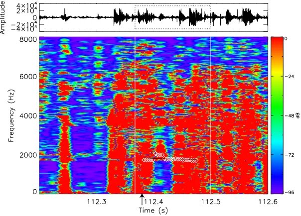
As noted above, the main reason for erroneous fitting was the overlap of more than two tweeks on the dynamic spectrum. The automated procedure cannot separate over-lapping tweeks. Figure 4 presents an example of a failed estimation, in which the fitting trace extends to the spec-tra of a few tweeks. In this case, the automatic estimation failed, while the manual method still gave reasonable
0
Fig. 5. Differencesδ(=automatic−manual) of the reflection heighth. Of the total tweeks, 61.0% fall in the range of−3 km< δ <3 km.
(Automatic - Manual) fc (Hz)
Number of tweeks
Fig. 6. Differencesδ(=automatic−manual) of the cut-off frequency for the first-order mode fc. Of the total tweeks, 59.7% fall in the range of −50 Hz< δ <50 Hz.
ues ofh(fc)anddof 88.83±0.24 km (1687.5±9.0 Hz) and
2816.0±39.0 km, respectively. In this case, the automatic procedure could not separate the target tweek (marked by the black arrow) from several other tweeks, incorrectly rec-ognizing all as one tweek. Such errors caused by over-lapping tweeks occurred in approximately 15% of the to-tal cases. For 72% of these error cases, d was less than 1000 km, which is smaller than typical values of tweekd
values. Thus, by checking the values ofd, we may be able to eliminate errors caused by overlapping tweeks.
Figures 5, 6, and 7 show the comparison results forh,
fc, andd, respectively, between the automated and manual
methods. The value of thex-axis indicates the maximum of the interval; in Fig. 5, for example, 0 is the maximum of the interval of−3 to 0 km. Out of 77 cases, acceptable values
ofh(−3 km< δ <3 km,δ=automatic−manual) and fc
(−50 Hz< δ <50 Hz) were obtained for 61.0% and 59.7%, respectively. We considered fc(h)to be acceptable if the
difference was less than±50 Hz (±3.0 km at∼1600 Hz), considering the spectral resolution of FFT (40 Hz). On the other hand, in Fig. 7, only 15.6% of the events have a difference indof less than 1000 km.
Comparing the results of the automated (for 194 tweeks, including 93 tweeks for which the manual method could not estimate parameters) and manual (for 77 tweeks) methods for the 2-minute averages, the averages and
standard deviations of h, fc, and d by the
auto-matic method (manual method) are 89.78±3.60 km
(89.20±2.68 km), 1672.2±68.5 Hz (1682.1±51.8 Hz),
-4000 -2000 0 2000 4000 6000 8000 10000
(Automatic - Manual) d (km)
Number of tweeks
Fig. 7. Differencesδ(=automatic−manual) in the propagation distance
d. Of the total tweeks, 29.9% fall in the range of−2000 km< δ <
11-Dec 13-Dec 15-Dec 17-Dec 19-Dec 21-Dec
UT
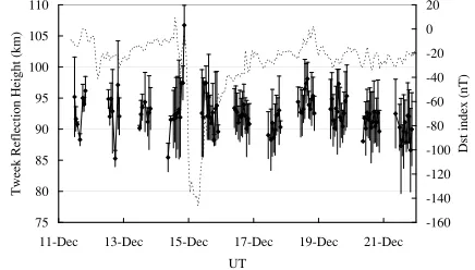
Fig. 8. Reflection height variations of tweeks estimated by the automatic procedure during a magnetic storm of 11–21 December 2006. The di-amonds with error bars indicate 2-minute averages and standard devia-tions of the reflection height. The dotted line indicates the variadevia-tions of theDstindex.
and 5429.9±2899.2 km (2371.0±1388.5 km), respectively. Thus, the differences (automatic − manual) between the mean h, fc, and d values are +0.58 km, −9.9 Hz, and
+3058.9 km, respectively. The difference forh(fc)is less
than the resolution of the FFT (40 Hz), but the difference in
dis very large and must be improved.
Figure 8 shows variations of tweek reflection heights ob-tained by the automatic procedure during an intense mag-netic storm on 11–21 December 2006. The plotted data are averages and standard deviations for 2-minute intervals ob-tained for each hour during nighttime. The total number of tweeks during the plotted interval was 918. For such a large number of tweeks, the automatic procedure is effec-tive in reducing the analysis time. The reflection heights abruptly rose in the initial phase (17:50–20:50 UT, 14 De-cember) (from 91.90 km to 106.72 km) and the recovery phase (9:50–12:50 UT, 15 December) (from 91.90 km to 97.43 km) of the storm. These increases in reflection height occur in response to the characteristic Dst variations, and
may indicate temporal decrease of energetic electron fluxes in the inner radiation belt.
4.
Conclusions
We have developed a procedure for automatic estimation of the reflection heighth(cut-off frequency of the first-order mode, fc), the propagation distanced, and the propagation
the differences of each ionospheric parameter between the automated and manual methods were+0.58 km,−9.9 Hz, and+3058.9 km for meanh, fc, andd, respectively. The
differences in h(fc)were sufficiently small and less than
the resolution of the FFT. These comparison results indi-cate that the developed procedure is a reliable method for automatically estimating tweek parameters and can be used to investigate long-term height variations of the D-region and lowerE-region of the ionosphere.
Acknowledgments. We are grateful to late K. Hidaka of the Kagoshima Observatory of the Solar-Terrestrial Environment Lab-oratory (STEL), Nagoya University, and M. Satoh, Y. Katoh, Y. Hamaguchi, and Y. Yamamoto of STEL for their technical sup-port of the continuous VLF/ELF measurements. This work was supported by Project 2 and the cooperative research program of STEL.
References
Bickel, J. E., J. A. Ferguson, and G. V. Stanley, Experimental observation of magnetic field effects on VLF propagation at night,Radio Sci.,5, 19, 1970.
Christian, H. J., R. J. Blakeslee, D. J. Bocchippio, W. L. Boeck, D. E. Buechler, K. T. Driscoll, S. J. Goodman, J. M. Hall, W. J. Koshak, D. M. Mach, and M. F. Stewart, Global frequency and distribution of lightnings as observed from space by the Optical Transient Detector,J. Geophys. Res.,108, ACL4-1–ACL4-15, 2003.
Davies, K.,Ionospheric Radio Waves, Waltham, MA: Blaisdell, 1969. Ferencz, O. E., Short impulse propagation in waveguides,Hiradastechnika
“Communications”,LIX,6, 2–6, 2004.
Ferencz, O. E., Cs. Ferencz, P. Steinbach, J. Lichtenberger, D. Hamar, M. Parrot, F. Lefeuvre, and J.-J. Berthelier, The effect of subiono-spheric propagation on whistlers recorded by the DEMETER satellite— observation and modeling,Ann. Geophys.,25, 1103–1112, 2007. Hayakawa, M., K. Ohta, and K. Baba, Wave characteristics of tweek
atmo-spherics deduced from the direction-finding measurement and theoreti-cal interpretation,J. Geophys. Res.,99, 10733–10743, 1994.
Hayakawa, M., K. Ohta, S. Shimakura, and K. Baba, Recent findings on VLF/ELF sferics,J. Atmos. Terr. Phys.,57, 467–477, 1995.
Holdsworth, D. A., R. Vuthaluru, I. M. Reid, and R. A. Vincent, Differen-tial absorption measurements of mesospheric and lower thermospheric electron densities using the Buckland Park MF radar,J. Atmos. Terr. Phys.,64, 2029–2042, 2002.
Lynn, K. J. and J. Crouchley, Night-time sferic propagation at frequencies below 10 kHz,Aust. J. Phys.,20, 101–108, 1967.
Maeda, K.-I., Study on electron density profile in the lower ionosphere,J. Geomag. Geoelectr.,23, 133–159, 1971.
Ohya, H., M. Nishino, Y. Murayama, and K. Igarashi, Equivalent electron densities at reflection heights of tweek atmospherics in the low-middle latitudeD-region ionosphere,Earth Planets Space,55, 627–635, 2003. Ohya, H., M. Nishino, Y. Murayama, K. Igarashi, and A. Saito, Using tweek atmospherics to measure the response of the low-middle latitude
D-region ionosphere to a magnetic storm,J. Atmos. Solar-Terr. Phys., 68, 697–709, 2006.
Outsu, J., Numerical study of tweeks based on waveguide mode theory,
Proc. Res. Inst. Atmos., Nagoya University,7, 58–71, 1960.
Shvets, A. V. and M. Hayakawa, Polarization effects for tweek propaga-tion,J. Atmos. Solar-Terr. Phys.,60, 461–469, 1998.
Thomas, L. and M. D. Harrison, The electron density distributions in the
D-region during the night and pre-sunrise period,J. Atmos. Terr. Phys., 32, 1–14, 1970.
Thomson, N. R., Experimental daytime VLF ionospheric parameters,J. Atmos. Terr. Phys.,55, 173–184, 1993.
Tohmatsu, T., Compendium of Aeronomy (translated and revised by T. Ogawa), Terra Scientific Pub. and Kluwer, 1990.
Yamashita, M., Propagation of tweek atmospherics, J. Atmos. Terr. Physics,40, 151–153, 1978.
Wait, J. R.,Electromagnetic Waves in Stratified Media, Pergamon, New York, 1972.