R E S E A R C H
Open Access
General optimization framework for surface
gateway deployment problem in underwater
sensor networks
Saleh Ibrahim, Manal Al-Bzoor
*, Jun Liu, Reda Ammar, Sanguthevar Rajasekaran and Jun-Hong Cui
Abstract
The performance of underwater sensor networks (UWSNs) is greatly limited by the low bandwidth and high propagation delay of acoustic communications. Deploying multiple surface-level radio-capable gateways can enhance UWSN performance metrics, reducing end-to-end delays and distributing traffic loads for energy reduction. In this paper, we study the problem of gateway placement for maximizing the cost-benefit of this UWSN architecture. We develop a mixed integer programming (MIP) gateway deployment optimization framework. We analyze the tradeoff between the number of surface gateways and the expected delay and energy consumption of the surface gateway architecture in the optimal case. We used an MIP solver to solve the developed optimization problem and integrated the optimal results to serve as an input for our simulations to evaluate the benefits of surface gateway optimization framework. We investigated the effect of acoustic channel capacity and the underwater sensor node deployment pattern on our solution. Our results show the significant advantages of surface gateway optimization and provide useful guidelines for real network deployment.
Keywords: Surface gateway, Multiple gateways, UWSN deployment, Deployment optimization
1 Introduction
An important component of oceanographic studies is the collection of data from the aquatic environment. Remote sensing has long been employed as a tool to collect aquatic data in underwater monitoring and exploration activities. Recently, in the last decade to be more specific, underwa-ter acoustic sensor networks (UWSNs) have emerged as a new alternative technology enabling underwater mon-itoring and exploration applications, including scientific, commercial, and military applications [1-5]. Compared to their remote-sensing counterparts, UWSNs have many advantages. UWSNs can provide localized and more pre-cise data acquisition. They can also employ a wider variety of sensors including, but not limited to, chemical, temper-ature, photo, and motion sensors.
UWSN technology is also replacing traditional under-water instrumentation technology. Traditionally, bulky sensor nodes equipped with data-storage capability are
*Correspondence: [email protected]
Department of Computer Science and Engineering, University of Connecticut, Storrs, CT 06269-2155, USA
manually deployed in the underwater target space. Each node operates independently for the duration of the mis-sion to collect readings according to a preset program. At the end of the mission, sensor nodes are picked up, and the collected data are retrieved and processed. UWSN tech-nology adds networking capabilities to underwater sensor nodes so that sensor nodes can relay real-time data to an off-shore or even an on-shore control station for imme-diate analysis. The communication channel can also be used to transmit control signals from the control station to the underwater sensor nodes, which enables interactive control of the underwater sensor network deployment. UWSNs offer many advantages over traditional instru-mentation techniques. First off, UWSNs add a real-time reporting functionality that enables a host of new real-time monitoring and warning systems. Another advantage of UWSN is that the sensing mission can be dynamically reconfigured without the need to physically access all the underwater nodes in order to reprogram them. While this particular feature makes the reuse of a UWSN deployment much less costly, it also provides for fixing configuration errors that compensates for unforeseen circumstances
and unexpected node failures. This improves the UWSN resilience compared to traditional instrumentation tech-niques. Therefore, sensor node failures can be detected soon after they occur, allowing early replacement or early abortion of the mission instead of having to wait until the end of the mission only to find that it has failed.
In addition to the usual design challenges faced by ter-restrial wireless sensor networks, UWSN technology has to deal with some unique challenges. It cannot use elec-tromagnetic waves for long-range communication due to their quick absorption in water. Acoustic waves are usually considered the practical solution for UWSN communica-tion. The dependency of UWSNs on underwater acoustic communications is particularly challenging. Factors such as the high levels of noise and the channel variability due to temperature, pressure, salinity gradients, and current-induced turbulence add more constraints to the already small bandwidth available for acoustic communication. Moreover, when the Doppler effect (due to mobility) is added to those factors, channel encoding becomes a crucial component to the success of underwater acous-tic sensor networks. However, the most limiting factor of underwater acoustic communications is the extremely low propagation speed of sound, which is roughly 1.5 km/s, subject to slight changes due to pressure, temper-ature, and salinity variations [6]. This is five orders of magnitude slower than the propagation speed of electro-magnetic waves. Such high propagation delay can cause high end-to-end delay, which could be greatly limiting for interactive applications and other monitoring applications where response time is critical.
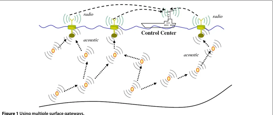
One way to mitigate the high propagation delay in acoustic communications is to deploy multiple surface-level gateways. In sensor networks, each sensor node can monitor and detect environmental events locally and then transfer these measurements through the network to a surface gateway node (also referred to as a sink in UWSNs), which then relays data to the control station. Unlike single-sink networks that use long underwater paths to reach the unique surface sink, in a multiple-sink underwater sensor network, as illustrated in Figure 1, underwater sensor nodes can send data packets toward their nearest surface gateway. A surface gateway then uses electromagnetic waves to forward the packets to the control station. Considering that electromagnetic wave propagation is in orders of magnitude faster than acoustic wave propagation, it is safe to assume that surface gate-ways can send packets to the control station in negligible time and with relatively small energy consumption since acoustic communications consume much more energy than radio communications [5]. In this way, all the surface gateways (or sinks) form a virtual sink. Although archi-tectures employing multiple surface gateway nodes were mentioned in [5,7], there is no formal study on surface
gateway deployment. Neither an analysis on the effect of using multiple surface gateways on the network energy consumption or delay characteristics has been conducted nor a guideline on the deployment of such a multi-sink architecture has been provided.
In this paper, we study the problem of surface gate-way deployment and present guidelines for deciding the number and locations of surface gateway nodes given an underwater sensor network deployment scenario. We focus on optimizing the cost of surface gateway deploy-ment, by finding the minimum number and the loca-tions of surface gateway nodes required to achieve a given design objective, which can be communication delay, energy consumption, fault tolerance, or a combina-tion of them. The surface gateway deployment problem is formulated as an optimization problem modeling the routing of data packets from underwater sensor nodes to the virtual sink under link capacity and flow conser-vation constraints. A variety of objective functions are presented. Our framework provides an optimal gateway selection from given gateway candidate locations which are assumed to be a given. The rest of this paper is organized as follows. In Section 2, we provide a review of related work. In Section 3, the network model and assumptions regarding the surface gateway deployment problem are presented and justified, and the surface gate-way deployment problem is formulated as an optimization problem. In Section 4, we evaluate our work, choosing sample problems to analyze the effect of various con-straints on the deployment solution quality, problem com-plexity, and feasibility. Finally, in Section 5, conclusions are drawn, and a future work is presented.
2 Related work
Figure 1Using multiple surface gateways.
The only research study in the frame of multiple sinks we found is [7], in which Seah and Tan investigated the use of multi-sink architecture to enhance the underwater sensor network reliability. In this study, the same message is directed to more than one of the multiple sinks, with the assumption that if any of the sinks gets the message, then it is considered delivered successfully. The simula-tion results showed that high-reliability benefits can be achieved at the cost of reasonable increase in energy con-sumption. The surface gateway (i.e., sink) deployment problem was not considered in this work. In a parallel research effort, [14] studied the problem of placing mul-tiple mobile data collectors in both delay-tolerant and delay-constrained underwater acoustic sensor networks. The authors defined candidate data collection stations as the maximal overlapping regions (MORs) of surface cir-cles corresponding to underwater node communication ranges. They developed anOn2lognalgorithm for find-ing MORs. An earlier work in [15] was the first to address the underwater surface gateway deployment problem and formulate it as an optimization problem. The problem of surface-level gateway placement has been addressed by later research effort in[16]. The authors used surface gate-ways deployment as a mean to guarantee connectivity and survivability (tolerance to single node failure). They pro-posed an approximation algorithm for choosing a minimal subset of candidate locations where SGs may be deployed. An effort by the authors in [17] addressed the deployment for a mobile multiple-sink architecture in UWSN. They used a prediction-based deployment strategy to cater for the mobility of underwater nodes. However, our work dif-fers from all above by formulating the problem to find the best candidate locations that satisfies a set of flow conservation constraints, interference constraints, num-ber of gateway constraints, and performance constraints
in addition to a set of delay and energy-consumption objectives.
3 Gateway deployment optimization generalized formulation
There are two approaches to handle the surface gateway deployment problem, (1) solving the underwater deploy-ment and the surface-level deploydeploy-ment problems jointly or (2) solving each of them separately. It is understood that solving both underwater and surface deployment prob-lems jointly will lead to optimal solutions that are better, or at least as good as, the outcome of the two-phase approach. However, since the objective of the research presented here is to analyze the effect of surface gate-way deployment on the overall underwater sensor net-work performance, we fix the underwater deployment and therefore opt for the latter option. Thus, we assume that there is a pre-existing underwater deployment that has been reached by a way or another.
The surface gateway deployment problem is formu-lated as a combinatorial graph optimization problem. The nodes of the graph represent underwater sensors and candidate surface gateway positions, and the problem is to find the subset of the candidate surface locations that maximizes a certain performance metric, satisfying a set of flow conservation constraints, interference con-straints, and a deployment cost constraint (on the number of surface gateways) or a performance constraint (such as maximum end-to-end delay or minimum reliability level).
to satisfy connectivity constraints as a precondition. This means that each underwater node has to have at least one connected path to one or more candidate surface loca-tions, taking into account the communication ranges of the involved intermediate nodes.
Associated with each underwater sensor node is a packet generation rate. Surface gateway nodes have to collect all generated data packets. The surface gateway deployment problem is formulated as a combinatorial optimization problem. The formulation consists of a basic set of constraints that can be augmented with a variety of objective functions.
3.1 Assumptions
The functionality of the UWSN considered is assumed to be mainly collecting data from underwater sensor nodes and transmitting the collected data samples at regular time intervals to a central station through one of the surface-level gateways. We assume that most of the traffic, therefore, will be flowing from the underwater nodes to the surface gateways. Inter-node communication (for pur-poses such as synchronization, collaborative sensing, data fusion, etc.) is assumed to be small enough to ignore.
Together, the set of surface-level gateways forms a vir-tual sinkfor the underwater sensors because the propaga-tion delay, the energy consumppropaga-tion, and the reliability of transmitting the received packet by a gateway to the cen-tral station over a direct or multi-hop radio path are far superior to underwater communication links. It is reason-able, therefore, to assume that a packet delivered to one of the surface gateways is delivered to the central station with high reliability and negligible delay and energy cost.
For simplicity, we assume that the data link protocol uses only fixed-length packets and that all links have the same bit rate. Consequently, the packet transmission time is consistent throughout the network, and if the transmission scheme is slotted, the packet transmission time is conventionally called the timeslot. Our deploy-ment formulation can be adjusted to include a variable packet length and a variable bit rate at different links without compromising the quality of the solution. This will require a pre-existing knowledge of these parame-ters which will increase number of inputs and will result in a more complex formulation of the flow constraints. However, we are interested in providing a more general-ized formulation of the gateway optimization problem to be adjusted and tuned for a more specified application that may require varying some of the inputs we assume is a fixed.
3.2 Definitions
The network is modeled as a graph, in which nodes rep-resent the underwater sensors and surface gateways, and edges represent pair-wise communication links.
3.2.1 Nodes
LetU be the set of all underwater sensor nodes andT be the set of candidate surface node positions.
LetVbe the set of all nodes, i.e.,
V=U∪T. (1)
Let Cv be the set of nodes within the communication
range of an underwater nodeu, i.e.,
Cu= {v:v∈V,v=u,d(u,v)≤RCu}, ∀u∈U, (2)
whered(v,w)denotes the Euclidean distance between the two nodesuandv, andRudenotes the maximum acoustic
communication range of the underwater nodeu.
3.2.2 Edges
Let the set of edgesEbe the set of all possible communi-cation links, i.e.,
E= {e(u,v):u∈U,v∈Cu}. (3)
LetEuOdenote the set of outgoing links of an underwater nodeu, i.e.,
EO
u = {e(u,v):v∈Cu}, ∀u∈U. (4)
Since surface gateways do not transmit data packets on their underwater acoustic interface,
EO
t =φ, ∀t∈T (5)
andEI
vdenote the set of ingoing links to a nodev, i.e.,
EI
v= {e(u,v):e(u,v)∈E}, ∀v∈V. (6)
3.2.3 Data generation and link flow rates
Letτ be the packet transmission time, called the times-lot in stimes-lot. Letgube the average packet generation rate at
nodeu∈U, i.e., the expected number of generated pack-ets during the packet transmission timeτ, and let Gbe the total data generation rate of the entire network, which should be equal to the average packet arrival rate at the virtual sink, i.e., the number of packets expected to arrive at the virtual sink during the packet transmission timeτ,
G=
u∈U
gu. (7)
Let fe be the average flow per packet time in edge e
measured in packets per packet time.
LetfvI be the average total flow into nodevper packet time, i.e.,
fvI = e∈EI v
fe, ∀v∈V. (8)
LetfO
u be the average total flow out of nodeuper packet
time
fuO=
e∈EO u
For gateways, there is no underwater outgoing flow, and therefore,
ftO=0, ∀t∈T. (10)
3.2.4 Gateway presence indicator
Letxtbe a binary variable that indicates whether a surface
gateway is to be deployed at candidate locationt, i.e.,
xt=
1 if a node deployed att,
0 otherwise , ∀t∈T. (11) 3.2.5 Link scheduling
LetTbe the schedule length, i.e., the number of time slots in a single period of the schedule.
Lethe,tbe a binary variable that indicates whether linke
is scheduled for transmission during slottof the schedule.
he(u,v),t=
1 utransmits tovat timeslott
0, otherwise ,
∀u∈U,e∈E, 0≤t<T.
(12)
3.2.6 Performance parameters
The most important performance aspects of any network are the delay and energy-consumption characteristics.
Delay Letυbe the average propagation velocity of sound waves in water.
LetτuP,vbe the propagation delay from nodeuto nodev. Thus,
τuP,v= d(u,v)
υ , ∀u∈U,v∈V. (13) LetτuQbe the average transmission queuing time includ-ing the expected channel access delay at nodeu.
Therefore, the total packet transmission delay,τu,v, over linke(u,v)is
τu,v=τuQ+τ+τuP,v, ∀u∈U,e∈EuO. (14) Energy consumption LetπeSbe the transmission energy required for transmitting one data packet over the under-water acoustic link e(u,v), πL be the listening/sleeping average energy consumption per packet time, andπvRbe the reception energy per packet. For surface gateways, the reception power is taken to include the energy required to forward a packet to the central station over radio.
Therefore, the total power consumptionπvof nodevper
packet time is
πv=πL+πvRfvI+ e∈EO v
πeSfe, ∀v∈V. (15)
Note that when the underwater sensor nodes use only one transmission power level πS, the total energy-consumption formula reduces to
πv=πL+πvRfIv+πSfvO, ∀v∈V. (16)
Due to the nature of the shared communication medium, contention for channel access can occur, and some transmission attempts may end up in failure. Trans-mission failures can also be caused by uncorrectable transmission errors. Let us assume that the transmission success probability on linkeis a constantρethat depends
on the channel utilization. This means that on the average,
a successful transmission will occur every 1 ρe
attempts.
The average number of retransmissions for linkeis hence
nesuch that
We assume that, on the average, every failed transmis-sion attempt will cost the sender πeS and will cost the receiverπvR. Including the energy cost of retransmissions, we get the following generalized formula for total power consumption:
Using any of above Equations 15, 16, and 18, the average energy consumed collectively by the network for a single transmission over linke(u,v)can be written as follows:
πe(u,v)=
The constraints can be classified into deployment con-straints, flow conservation concon-straints, and interference constraints.
3.3.1 Deployment constraints
• Number of surface gateways
If the objective of the optimization is to minimize delay or energy consumption using a limited number of surface nodes,N, the following constraint can be used to limit the number of gateways deployed to at mostN:
t∈T
xt≤N. (20)
• Gateway presence indicator constraints
No more than one gateway can be deployed at any candi-date location:
xt∈ {0, 1}, ∀t∈T. (21)
3.3.2 Flow constraints
underwater sensor nodes and through the network to a common sink station. Therefore, the analysis is limited to the (possibly multi-path) route from each underwater sen-sor to the virtual sink. Control traffic flowing from the central station down to the underwater sensor nodes or inter-node traffic for the purpose of synchronization or localization or other functions than sensing data transfer will be ignored.
• Gateway presence constraints
Data can only be received at locations where surface gateways are deployed. This constraint can be written as follows:
ftI≤xtG, ∀t∈T. (22)
This means that the total flowftI into candidate gateway locationthas to be zero ifxt =0; otherwise,ftIcan grow
as large as the maximum potential flow in any link in the network which is equal to the total data generation rateG
in the network, thus rendering the constraint void.
• Per-node flow conservation constraints
Flow conservation implies that for underwater sensor nodes, the sum of the average flows leaving a node equals the sum of the flows entering that node plus the local data generation rate.
fuO−fuI=gu, ∀u∈U. (23)
• End-to-end flow conservation constraints
Flow conservation also implies that the total data genera-tion rate of all underwater nodes must equal the total data absorption rate by the virtual sink composed of all surface gateways since each packet, generated by any source, must eventually be received by a surface node (before being relayed to the sink).
t∈T
ftI =G. (24)
• Flow allocation constraints
The average flow in any edgeeduring a schedule period cannot exceed the total number of time slots in which the link is active
T·fe≤ T
t=1
he,t
, ∀e∈E. (25)
Note that since we assume the schedule is periodic, there is no need to add a constraint to enforce the recep-tion of a packet before sending it out. If a packet is sent before being received, this means that it was stored from the previous period. It follows that the maximum per-hop queuing delay will not exceedT−1 timeslots.
3.3.3 Interference constraints
Because they use a shared medium to communicate, each node will be able to utilize only a fraction of the under-water channel bandwidth. The exact formulation of inter-ference constraints will depend heavily on the medium access control protocol being used by the UWSN. With-out knowing the specifics of the medium access protocols, we can assume a randomized protocol with either one of two medium access schemes, namely slotted vs. unslot-ted schemes. It has been shown in literature that due to the relatively high propagation delay of acoustic sig-nals, slotted protocols behave as inefficiently as unslotted protocols do [19-22]. Therefore, we can assume that the channel utilization cannot exceed the theoretical maxi-mum of approximately 0.18. Letbbe the channel bit rate. We define the effective bandwidthBas the throughput at the maximum utilization. Hence,
B≤0.18b. (26)
To avoid collision at the receiver, a node is able to receive successfully only if (1) it is not transmitting and (2) all nodes that are within its interference range are silent for the duration of the reception. To formulate this constraint, we first define the interfering node set Iv for receiverv
as the set of nodes whose transmissions can potentially collide with data packets sent to receiverv. Thus,
Iv=
u:u∈U,d(u,v)≤RIu, ∀v∈V. (27) A pessimistic formulation of the effect of contention on constraining the available bandwidth for each receiverv
can be written as follows:
fvO+ u∈Iv
fuO≤B, ∀v∈V. (28)
This formulation is called pessimistic because that assumes that transmissions that could interfere with the reception at nodevare going to happen in distinct time intervals without any overlapping. This is the worst case because it leaves the minimum possible bandwidth for
v to receive its own intended transmissions. In reality, however, some of these transmissions from interfering neighbors of nodevcan occur simultaneously and suc-cessfully. Consider, for instance, two interfering neighbors ofv, calledu1andu2,vcannot receive any signals as long
as it can hear either u1or u2 is transmitting. Now, ifu1
andu2are sending tow1andw2, respectively, it is possible
that both transmissions can succeed simultaneously ifu1
is not withinw2’s interference range andu2is not within w1’s interference range.
Because surface nodes do not transmit data packets underwater, the interference constraint formula for sur-face gateways reduces to
u∈It
For each underwater node in the interfering node set of a certain receiver, we define thevulnerable slotsof a link
e=(u,v)with respect to a transmitterwas follows:
This means that node u cannot send to nodev during slot t if node w is transmitting during time slots t =
(t−i)moduloT,∀i∈Pu,v,w. Note thatt−icould be
neg-ative, which means that there is potential interference with packetswsends during earlier schedule periods. There-fore, we write the interference avoidance constraint as follows:
h(u,v),t≤1−h(w,z),t, t=(t−i)moduloT, ∀(u,v)∈E,w∈Iv.
(w,z)∈EwO,i∈Pu,v,w, t∈ {1,. . .,T}
(31)
In addition, we have to prevent self-interference by enforcing the following constraint:
e∈EO v
he,t≤1, ∀v∈U,t∈ {1,. . .,T}. (32)
This means that a node cannot transmit on more than one link during the same time slot.
Tis the number of time slots a packet spends waiting in the transmission queuing at any node. Since the queuing delay can vary from 0 up toT −1 time slots, we estimate
L= T−21. In order to for this estimate to be accurate and in order to insure the best possible performance, a search for the minimum feasible schedule length will be neces-sary. We do so following the method pointed out in [13]. Namely, we formulate the problem starting fromT = 2 and attempt to solve the MIP problem. As long as the MIP is infeasible, we continue to increase the schedule lengthTuntil we find the minimumT for which the ILP formulation is feasible.
3.4 Objective functions
The objective function determines the goal of the deploy-ment optimization. In general, the objective can be (1) a collective measure, such as minimizing the aver-age end-to-end delay and minimizing the total energy-consumption rate or (2) an extreme measure, such as minimizing the worst case end-to-end delay or maximiz-ing the worst case node lifetime.
3.4.1 Minimizing expected end-to-end delay
The objective here is to minimize the expected end-to-end delay for all packets. The end-to-end-to-end-to-end delay for a packet is the sum of the per-hop delay over the entire path from the source that generates the packet to virtual sink (i.e., the gateway) that receives it. As expressed earlier in
Equation 14, the per-hop delay consists of three compo-nents: queuing and channel access delays, transmission time, and propagation delay. LetKu,tbe the set of all active
paths from source underwater nodeuto surface gateway candidate locationt. Let ki = (e1,e2,· · ·,em)be one of
ki. It follows that the average end-to-end delay betweenu
andtis
The flow in each link in terms of the path flows can be written as follows:
Let δe,ki be a set of decision variables that indicate whether linkeis part of pathk, i.e.,
δe,ki=
1,e∈ki
0, otherwise. (36)
Using Equation 36, Equation 35 can be rewritten as follows:
The average end-to-end delay betweenuand the virtual sink (all surface gateway candidate location) is
E
Now, the overall expected end-to-end delay can then be written as:
Using Equations 35, 36, 33, and 7, the overall expected end-to-end delay can be rewritten as follows:
E
Also, the corresponding objective function will be
3.4.2 Minimizing expected energy consumption
The objective is to minimize the expected end-to-end energy consumption, i.e., the energy consumed in the net-work for a packet to travel from its source to a sink. The average energy,πe, consumed collectively by the network
in order to transmit one packet on linkewas formulated in Eqaution 19. The expected end-to-end per packet energy consumption for a pathki ∈ Ku,tbetween source nodeu
and sinktcan be written as
πkE i=
e∈ki
πe, ∀u∈U,t∈T,ki∈Ku,t. (42)
Following a derivation similar to that given in subsec-tion 3.4.1, the overall expected end-to-end per packet energy consumption can be shown to be
E[πE]= 1
Also, the corresponding objective function will be
Minimize
3.4.3 Minimizing worst case per-source average delay When the optimization objective is to minimize the over-all average end-to-end delay, some sources maybe exces-sively penalized with a much longer delay. In monitoring applications where uniform response time is favored, the optimization objective has to be minimizing the worst case, per-source average delay. In other words, the objec-tive is to minimize the average delay observed by packets from each source taken separately, to guarantee the best possible worst case scenario. In order to define this objec-tive, we define a set of new flow variables,fe,u to denote
the portion of the flow in linkethat is generated originally by nodeu. If no path fromuto the virtual sink uses linke, this implies thatfe,u=0.
The flow conservation constraints can be rewritten to be source specific as follows:
The end-to-end per-source average delay τuE can be written as follows:
We define an upper boundUτfor the per-source average delay,
τuE≤Uτ. (47)
Also, the optimization objective is to minimize this upper bound,
Minimize{Uτ}. (48)
4 Performance evaluation
We conducted extensive simulation to evaluate our gate-way deployment optimization framework. We assumed that acoustic transceivers of all nodes, both underwa-ter nodes and surface gateways, to be homogeneous and, therefore, the communication range is assumed to be con-stant for all nodes. We assume that sensor nodes are either stationary or that their motion is correlated strongly enough to assume that their relative locations are fixed. We adopt the pessimistic interference model. To reduce the problem complexity, we assume a lightly loaded, i.e., such that channel access delays and queuing delays can be safely ignored. Since both channel access delay and queu-ing delay are functions of network load (i.e., flow), keepqueu-ing the network very lightly loaded justifies the assumption that the queuing delay is constant, hence allowing the lin-earization of the formulation and the use of LP solvers. When the load is increased, the non-linear formulation can be solved similarly by piece-wise linearization algo-rithms, such as the Frank-Wolfe algorithm. Although the problem can be solved for a choice of optimization goals, we limit our focus on the simplest optimization goals, namely minimizing the average delay and minimizing the average power consumption. The LP solver uses a brute-force search algorithm to find the optimal gateway deployment locations by numerating all possible candi-date solutions and checking whether each satisfies the problem’s statement.
4.1 Case study
In order to evaluate the benefits and the performance of the gateway deployment optimization techniques, we used the following simulation setting.
Throughout the experiments, we fixed the packet length
L= 400 bits, the underwater acoustic propagation velocity υ= 1.5 km/s, and the transmission power is set to a con-stant of 1 W/s per packet time. The communication range for the underwater modems for all nodes is fixed atRC= 150. We also fixed the area of deployment to a square area of 600 m×600 m horizontal extent and fixed the candi-date gateway deployment positions to a 5×5 square mesh of points spaced 150 m apart .
0 100 200 300 400 500 600 700m 0
100 200 300 400 500 600 700 800m
Surface Candidate Positions
Underwater Sensors at 100m depth
Figure 2Uniform deployment.
regardless of its horizontal location, is within the commu-nication range of at least one surface gateway candidate position, thus satisfying the connectivity requirement. This guarantees that an optimal solution can be found by setting a large-enough limit on the number of sur-face gateway nodes,N. Finally, the data generation rate at each underwater sensor is set to 1 packet per second. The acoustic channel effective bit rateBis varied among 5, 10, and 50 kbps. Accordingly, the packet transmission time τ =80, 40, and 8 ms, respectively, and the data generation rateg=0.08, 0.04, and 0.008 packets per packet time, and the energy consumption per packet transferπS =80, 40, and 8 W, respectively.
4.2 Results
To characterize the benefits and limitations of the deploy-ment of surface gateways, we analyze the effect of the following factors:
• Number of gateway nodes
When the number of allowed surface-level gateway nodes increase, the performance characteristics, average delay or
0 100 200 300 400 500 600 700m
0 100 200 300 400 500 600 700 800m
Surface Candidate Positions
Underwater Sensors at 100m depth
Figure 3Random deployment (uniformly random).
0.1 0.12 0.14 0.16 0.18 0.2 0.22 0.24 0.26 0.28
0 5 10 15 20 25
Delay (s)
Number of Gateway Nodes B=50kbps B=10kbps B=5kbps
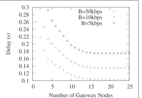
Figure 4Average delay, uniform underwater deployment.
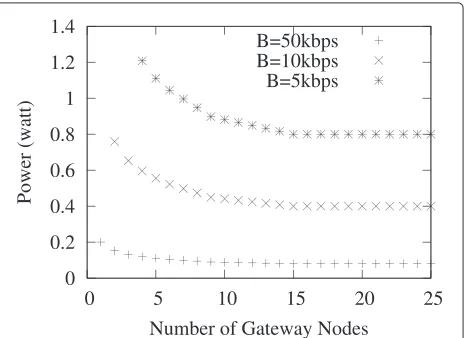
average power consumption, is expected to improve. To verify that, we vary the number of allowed surface nodes from 1 to 25 nodes and solve the optimization problem to get the optimal average delay or energy. Results show that an increase in the number of surface gateways can dramat-ically enhance performance, especially when the network is lightly loaded.
• Network load
Intuitively, when the ratio of total data generation rate to the per-node channel bandwidth increases, the min-imum number of surface-level nodes required to make the problem feasible increases. This is due to the fact that surface gateways will saturate with incoming traf-fic and, therefore, more nodes will be needed to handle the additional traffic corresponding to the increased data generation rate. On the other hand, increasing channel capacity reduces the network load, and consequently, our assumptions about ignoring queuing delays become more
0 0.2 0.4 0.6 0.8 1 1.2 1.4
0 5 10 15 20 25
Power (watt)
Number of Gateway Nodes B=50kbps B=10kbps B=5kbps
0.1 0.12 0.14 0.16 0.18 0.2 0.22 0.24 0.26 0.28 0.3
0 5 10 15 20 25
Delay (s)
Number of Gateway Nodes B=50kbps B=10kbps B=5kbps
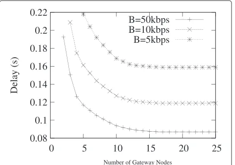
Figure 6Average delay, random underwater deployment.
realistic. To demonstrate the effect of channel capacity on the quality of the solution, we solve the deployment opti-mization problem for different link capacities, namely 5, 10, and 50 kbps.
• Underwater deployment pattern
If the set of candidate surface gateway positions is pre-set, the locations of underwater sensors and the distri-bution of data generation load among them are expected to affect the benefit of adding more surface gateways. If underwater sensors are clustered in groups, less surface gateways are expected to feasibly route all traffic to the surface, compared to the case when underwater sensors are spread evenly over the deployment area. On the other hand, clustering increases the odds of collision and, in the case of high traffic loads, can negatively affect delay and energy consumption. To study the effect of the deploy-ment scheme of the given set of underwater sensors on the
0 0.2 0.4 0.6 0.8 1 1.2 1.4
0 5 10 15 20 25
Power (watt)
Number of Gateway Nodes B=50kbps B=10kbps B=5kbps
Figure 7Average energy, random underwater deployment.
0.12 0.14 0.16 0.18 0.2 0.22 0.24 0.26 0.28 0.3
0 5 10 15 20 25
Delay (s)
Number of Gateway Nodes Uniform Random
Figure 8Average delay, uniform vs. random underwater deployment.
result of the surface gateway deployment optimization, we use two underwater deployment patterns.
The uniform underwater deployment was chosen because the uniformity of the solution simplifies the process of verifying the results. The chosen underwater deployment consists of a 7 × 7 planar mesh of sen-sor nodes. The distance between two adjacent nodes is 100 m, and therefore, the nodes cover the entire 600 × 600-m area. This problem setting is illustrated in Figure 2.
It was similar to the uniform underwater deployment, except that the 49 underwater sensor nodes are dis-tributed at random within the 600× 600-m underwater area. This problem setting is illustrated in Figure 3.
4.2.1 Effect of number of gateway nodes
Results show that an increase in the number of sur-face gateways can dramatically enhance performance,
0.4 0.5 0.6 0.7 0.8 0.9 1
0 5 10 15 20 25
Power (watt)
Number of Gateway Nodes Uniform Random
0.08 0.1 0.12 0.14 0.16 0.18 0.2 0.22
0 5 10 15 20 25
Delay (s)
Number of Gateway Nodes
B=50kbps B=10kbps B=5kbps
Figure 10Average delay, random underwater deployment experiment 2.
especially when the network is lightly loaded. For example, Figure 4 shows that the expected delay corresponding to
B= 50 kbps can be reduced from 0.26 to 0.16 s using four surface gateways instead of one. It is also worth noting that the improvement gained by adding a surface gateway diminishes as the number of surface gateways increase. After a certain number of surface gateways, depending on underwater deployment and other factors, any additional surface nodes have negligible effect on the performance of the network. This is due to the fact that at that point, all underwater nodes communicate with the a surface gate-way at the candidate position nearest to each of them, and therefore, further addition of surface nodes becomes redundant.
4.2.2 Effect of network load
Simulation results show that the performance improve-ment resulting from the addition of more surface gateway
0 0.2 0.4 0.6 0.8 1 1.2
0 5 10 15 20 25
Power (watt)
Number of Gateway Nodes B=50kbps B=10kbps B=5kbps
Figure 11Average energy, random underwater deployment experiment 2.
0.08 0.1 0.12 0.14 0.16 0.18 0.2 0.22 0.24
0 5 10 15 20 25
Delay (s)
Number of Gateway Nodes B=50kbps B=10kbps B=5kbps
Figure 12Average delay, random underwater deployment experiment 3.
nodes diminishes when the network load increases, con-firming our expectations as explained before. For example, Figure 5 shows that the heavily loaded network, corre-sponding to the channel capacity of 5 kbps has a smaller dynamic range of 0.2/0.08 = 2.5 than the lightly loaded network corresponding toB= 50 kbps, whose dynamic range is equal to 1.2/0.8 = 1.5. Figures 4 and 5 show the effect of varying the channel capacity, in the case of uniform underwater deployment, on the expected delay and expected energy consumption, respectively. Figures 6 and 7 show the effect of varying the channel capac-ity in the case of random underwater deployment, on the expected delay and expected energy consumption, respectively.
4.2.3 Effect of underwater deployment pattern
Figures 8 and 9 compare the results of the uniform underwater deployment case and the random underwater
0 0.2 0.4 0.6 0.8 1 1.2
0 5 10 15 20 25
Power (watt)
Number of Gateway Nodes B=50kbps B=10kbps B=5kbps
deployment case at a fixed channel capacity of 10 kbps. When the number of surface gateways is small, the ran-domly distributed underwater deployment suffers more congestion and therefore performs slightly poorer than the uniformly distributed counterpart in both delay and energy-consumption metrics. When the number of sur-face gateways increases, the effect of congestion dimin-ishes, and the effect of clustering grows stronger. After a certain number of surface gateways, the energy con-sumption of the randomly distributed underwater deploy-ments converges to that of the uniformly distributed case because, eventually, each underwater node becomes one hop away from a surface gateway. Although Figure 8 shows that the delay of the randomly distributed case eventually becomes lower than the uniformly distributed case is not necessarily always true. The problem instance shown in Figure 3 happened to have an average dis-tance between underwater nodes and candidate surface positions, lower than that in the uniformly distributed case in Figure 2, and therefore, the randomly distributed underwater deployment case exhibits less average prop-agation delay. The experiments were repeated for sev-eral random underwater deployments to confirm that the results exhibit the same trends. Figures 10, 11, 12 and 13 illustrate two more samples for the random deployment results.
5 Conclusions
In this paper, we provided a generalized optimization framework for the surface gateway deployment prob-lem. We demonstrated how to use the formulation to find the optimal placement of surface gateways with respect to a variety of optimization goals and a set of flow conservation constraints, interference constraints, and deployment constraints. We assisted our work by incorporating the optimal gateway optimization frame-work results in simulating the operation of the UWSN with multiple surface gateways. Our simulation results confirmed the potential for performance improvement using multiple surface gateways, such as reducing both average delay and energy consumption. It was also shown that the effect of the added surface gateways depends on the channel capacity or the network loading level, as well as the given underwater sensor deployment pattern. Our work presented here helps to pave the way for a wide variety of future research. One possible improve-ment is to optimize underwater and surface deployimprove-ments jointly. Another is to consider mobility of surface gateways and a static UWSN with some level of location certainty models and integrate it as a new design parameter in our framework.
Competing interests
The authors declare that they have no competing interests.
Acknowledgements
This work is supported in part by the US National Science Foundation under CAREER grant nos. 0644190, 1018422, 1127084, 115213, and 1205665.
Received: 6 December 2012 Accepted: 30 April 2013 Published: 13 May 2013
References
1. G Xie, J Gibson,A Networking Protocol for Underwater Acoustic Networks. (CS Department, Naval Postgraduate School Operations Research Department Monterey, CA 93943, 2000)
2. JG Proakis, EM Sozer, JA Rice, M Stojanovic, Shallow water acoustic networks. IEEE Commun. Mag.39(11), 114–119 (2001)
3. IF Akyildiz, D Pompili, T Melodia, Underwater acoustic sensor networks: research challenges. Ad Hoc Netw.3(3), 257–279 (2005)
4. J Heidemann, Wei Ye, J Wills, A Syed, Yuan Li, inProc. of IEEE Wireless Communications and Networking Conference, WCNC 2006. Research challenges and applications for underwater sensor networking (Las Vegas, 3–6 April 2006)
5. JH Cui, J Kong, M Gerla, S Zhou, The challenges of building scalable mobile underwater wireless sensor networks for aquatic applications. IEEE Netw.20(3), 12–18 (2006)
6. L Berkhovskikh, Y Lysanov,Fundamentals of Ocean Acoustics. (Springer-Verlag, Berlin Heidelberg, 1982)
7. WKG Seah, HP Tan, inProc. of the First International Conference on Integrated Internet Ad Hoc and Sensor Networks, InterSense 2006. Multipath virtual sink architecture for wireless sensor networks in harsh
environments (Nice France, 30–31 May 2006)
8. MF Younis, K Akkaya, Strategies and techniques for node placement in wireless sensor networks: a survey. Ad. Hoc. Netw.6(4), 621–655 (2008) 9. B Hao, H Tang, G Xue, inProc. of IEEE workshop on High Performance
Switching and Routing, HPSR 2004. Fault-tolerant relay node placement in wireless sensor networks: formulation and approximation (Phoenix, 2004), pp. 246–250
10. Y Hou, Y Shi, HD Sherali, SF Midkiff, On energy provisioning and relay node placement for wireless sensor networks. Wireless Commun. IEEE Trans.4(5), 2579–2590 (2005)
11. Q Wang, K Xu, G Takahara, H Hassanein, inProc. of IEEE Global Telecommunications Conference, GLOBECOM 2005. Locally optimal relay node placement in heterogeneous wireless sensor networks (St. Louis, 2005)
12. D Pompili, T Melodia, IF Akyildiz, inProc. of First ACM International Workshop on Underwater Networks, WUWNet 2006. Deployment analysis in underwater acoustic wireless sensor networks (Los Angeles, 25 September 2006), pp. 48–55
13. L Badia, M Mastrogiovanni, C Petrioli, S Stefanakos, M Zorzi, inProc. of First ACM International Workshop on Underwater Networks, WUWNet 2006. An optimization framework for joint sensor deployment, link scheduling and routing in underwater sensor networks (Los Angeles, 25 September 2006) 14. W Alsalih, H Hassanein, S Akl, inProc. of IEEE Local Computer Networks
Conference, LCN 2008. Delay constrained placement of mobile data collectors in underwater acoustic sensor networks (Montreal, 14–17 Oct 2008), pp. 91–97
15. S Ibrahim, JH Cui, RA Ammar, inProc. of IEEE Military Communications Conference, MILCOM 2007. Surface-level gateway deployment for underwater sensor networks (Orlando, 29–31 Oct 2007), pp. 1–7 16. S Misra, SD Hong, G Xue, J Tang, Constrained relay node placement in
wireless sensor networks: Formulation and approximations. IEEE/ACM Trans. Netw.18(2), 434–447 (2010)
17. J Liu, X Han, M Al-Bzoor, M Zuba, JH Cui, RA Ammar, S Rajasekaran, inProc. of IEEE Symposium on Computers and Communications, ISCC 2012. PADP: Prediction assisted dynamic surface gateway placement for mobile underwater networks (Cappadocia, 1–4 July 2012)
18. S Ibrahim, RA Ammar, JH Cui, inProc. of IEEE Symposium on Computers and Communications, ISCC 2009. Geometry-assisted gateway deployment for underwater sensor networks (Sousse, 5–8 July 2009)
20. S De, P Mandal, SS Chakraborty, On the characterization of Aloha inunderwater wireless networks. Math. Comput Model.53, 2093–2107 (2011)
21. AA Syed, W Ye, J Heidemann, B Krishnamachari, inProc. of the second workshop on Underwater networks, WuWNet 2007. Understanding spatio-temporal uncertainty in medium access with ALOHA protocols (Montereal, 2007), pp. 41–48
22. JH Gibson, GG Xie, Y Xiao, H Chen, inProc. of MTS/IEEE Oceans 2007 Conference. Analyzing the performance of multi-hop underwater acoustic sensor networks (Scotland, June 2007)
doi:10.1186/1687-1499-2013-128
Cite this article as:Ibrahimet al.:General optimization framework for
surface gateway deployment problem in underwater sensor networks. EURASIP Journal on Wireless Communications and Networking20132013:128.
Submit your manuscript to a
journal and benefi t from:
7Convenient online submission 7Rigorous peer review
7Immediate publication on acceptance 7Open access: articles freely available online 7High visibility within the fi eld
7Retaining the copyright to your article