Comparative Assessment of Ammonia Emissions from Potential Environmentally Superior Technologies for Swine Facilities

ABSTRACT

SEMUNEGUS, HILAWE. Comparative Assessment of Ammonia Emissions from Potential Environmentally Superior Technologies for Swine Facilities (Under the direction of Dr. S. Pal Arya and Dr. Viney P. Aneja)

Globally, domestic animal waste contributes nearly half of the total tropospheric

ammonia (NH3) emitted into the atmosphere. In North Carolina, swine waste from agricultural operations represents 47% of the total ammonia emissions and 21% of the state’s

nitrogen budget. Due to the short residence time of NH3 (1-5 days) in the atmosphere, deposition occurs close to emission sources. Ammonia that does not deposit quickly

combines with acidic species such as sulfuric acid, nitric acid, and hydrochloric acid to form

ammonium aerosols. Ammonium aerosols travel farther from emission sources due to their

lower deposition velocity leading to longer residence time (1-15 days) compared to gaseous

ammonia. Detrimental effects of high concentrations and dry and wet depositions of reduced

N species include harmful algal blooms, nitrogen enrichment, and eutrophication in aquatic

ecosystems, soil acidification, and respiratory damage due to exposure of fine particulate

matter (PM 2.5) formation, nitrogen saturation of forest soil, odor emanation, and visibility

degradation.

In response to perceived adverse environmental impacts of the nearly 10 million hogs

residing in North Carolina, alternative waste treatment methods were evaluated that could

potentially reduce substantial emissions of ammonia. These are being evaluated by the OPEN

Project Team. This study was a part of that evaluation, especially focusing on the ammonia

emissions from two potential environmentally superior technologies (ESTs). Between April

with two conventional Lagoon and Spray Technology (LST) facilities, which were also

sampled during different seasons. The two alternative technologies are (1) The Covered

In-Ground Ambient Digester Technology and (2) The Constructed Wetlands/Solid Separator

Technology. Using the dynamic flow-through chamber system, ammonia flux measurements

were determined, along with measurements of meteorological parameters such as wind speed

and direction, air temperature, relative humidity, and solar radiation from a 10 m tower at all

the EST and LST sites.

For LST sites, the average ammonia fluxes for the storage ponds were 2,385 µg NH3 -N/m2/min for Stokes Farm and 1,657 µg NH3-N/m2/min for Moore Farm during the fall season measurement campaigns. For winter season measurement campaigns, average

ammonia flux measurements were 153 and 325 µg NH3-N/m2/min for the storage ponds at Stokes and Moore farms, respectively. For the April and November 2002 measurement

campaigns at Barham Farm (EST), respectively, the average ammonia fluxes from the liquid

waste storage ponds were 1,169 µg NH3-N/m2/min and 352 µg NH3-N/m2/min. At Howard Farm (EST), average measured ammonia fluxes were 790 µg NH3-N/m2/min and 243 µg NH3-N/m2/min during the June and December 2002 field campaigns.

Using the mass balance method, NH3-N emissions from conventional LST or baseline sites were compared with those from ESTs. Ammonia emissions from different components

such as liquid waste storage ponds, hog barns, and spray fields were also evaluated. To

predict baseline NH3-N emissions during the EST measurement periods, lagoon temperature (TL) and air temperature – lagoon temperature difference (D) were inserted into an observational statistical model, developed from all baseline measurements. The observational

Log10(Area*flux/ton) = 3.8655 + 0.0449*TL – 0.05946*D where TL and D are in oC and Area*flux/ton represents the NH3-N emissions from the lagoon per 1000 kg of live animal weight (LAW), expressed in units of µg NH3-N/1000 kg-LAW/min. Emissions of NH3-N normalized by the nitrogen excretion rate show that the Constructed Wetlands/Solid

Separator Technology was not effective at all in reducing nitrogen emissions compared to the

conventional Lagoon and Spray Technology. The Covered In-Ground Ambient Digester

COMPARATIVE ASSESSMENT OF AMMONIA EMISSIONS FROM POTENTIAL ENVIRONMENTALLY SUPERIOR TECHNOLOGIES FOR SWINE FACILITIES

by

HILAWE SEMUNEGUS

A thesis submitted to the Graduate Faculty of North Carolina State University

In partial fulfillment of the Requirements for the Degree of

Master of Science

DEPARTMENT OF MARINE, EARTH AND ATMOSPHERIC SCIENCES

Raleigh

2003

APPROVED BY:

_____________________________ ___________________________ S. Pal Arya Viney P. Aneja

Chair of Advisory Committee Co-Chair of Advisory Committee

BIOGRAPHY

Hilawe Semunegus was born on October 22, 1977, in Addis Ababa, Ethiopia to Dr.

Semunegus Hailemariam and Tsega Berecket. Upon leaving Ethiopia with his family as a

political asylee at the age of seven, Hilawe attended four different elementary schools and

two different middle schools while his family moved around in Raleigh, NC. During the

eighth grade, Hilawe lived with his parents for a year in Hanoi, Vietnam and during his

sophomore year in high school, he moved to Bangladesh for three years with his parents and

attended the American International School at Dhaka.

Upon graduating from high school in 1995, Hilawe entered North Carolina State

University and graduated in May 2001, with a B.S. in Environmental Sciences with an Air

Quality Concentration. While pursuing a B.S. at North Carolina State University, Hilawe was

Student Patrol Director for the NCSU Campus Police for four years where he supervised up

to 20 employees and was responsible for providing safety escorts for faculty and students of

the university.

In the fall of 2001, Hilawe entered the Graduate School at North Carolina State

University to study Atmospheric Sciences. While attending NCSU, Hilawe worked as a

teaching assistant, meteorology lab instructor, and research assistant. In August of 2002,

Hilawe was awarded a NOAA Education Partnership Program Scholarship as a Graduate

Scientist, which provided training for permanent employment with the National Oceanic and

Atmospheric Administration/National Climatic Data Center (NOAA/NCDC) in Asheville,

NC, upon his graduation with a M.S. in Atmospheric Sciences. Between March 30 and April

Florida A&M University in Tallahassee, Florida, where he placed first overall, among 80

participants from several universities, in the graduate student poster presentation competition.

Presently, Hilawe is preparing to start his employment with the National Climatic

Data Center in Asheville as a Physical Scientist. He will be working on satellite data,

collected as part of the International Satellite Cloud Climatology Project (ISCCP), to study

the effects of clouds on the radiation balance with emphasis on further understanding the

ACKNOWLEDGEMENTS

This research was funded by the Animal and Poultry Waste Management Center of

North Carolina State University. I would like to thank my Graduate Advisory Committee

members, Dr. S. Pal Arya, Dr. Viney P. Aneja, Dr. Sethu Raman, and Dr. John J. Bates for

providing me with the opportunity to pursue my M.S. degree and for their encouragement,

support, and guidance. I would also like to thank Dr. Deug-Soo Kim who managed and

guided my field research and always made time to help me with any questions or problems I

had. My sincere appreciation goes out to the Program OPEN statisticians, Dr. Dave Dickey

and Dr. Len Stefanski, who were both kind enough to offer me a “crash course” in using the

SAS software and also for assisting me with statistical analysis of my data. I give many

thanks to Lynn Worley-Davis who always manages to come through despite all the obstacles

she faces while organizing field campaigns. Many thanks to Dr. Sethu Raman and Ryan

Boyles, at the State Climate Office of North Carolina, who graciously provided me with

climatology data for my research.

I would like to thank Chantell Haskins, Jacqueline Rousseau, Sabrina Tucker, and Ivy

Washington from the NOAA Educational Partnership Program and Colleen Babcock and

Jennifer Garren from the Oak Ridge Institute of Science and Education (ORISE) for

affording me the opportunity to serve as a Graduate Scientist. I am also grateful to Mark

Yirka of the North Carolina Division of Air Quality for providing me with technical support,

usually on short notice, with the operation of the ammonia detection instruments. I owe a

great deal of gratitude to Brian Baldelli at Machine and Welding Purity Gases who hauled

The Air Quality Research Group members, Jessica Blunden, Heather Arkinson, Dr.

Sharon Phillips, Dr. Quansong Tong, Binyu Wang, Dongmei Yang, Kanwardeep Bajwa, Ian

Rumsey, Zach Holmes, and Damon Sandor, provided me with friendship, support and

assistance in my two years as a Master’s Student at NCSU and I am honored to have known

such a group of people. Many thanks to Damon Sandor who helped me with field research

while I was attending classes. I would like to offer a special thank you to Jessica Blunden

who showed me true friendship and unconditional support along the way and continues to do

so. I am also very appreciative of all the graduate students in the department who were

always supportive. Thank you to Michele Kephart, Beth Graf, Connie Hockaday, Susan

Curtis, Tim Wright, Jennifer Cash, Alison Diehl, and Brenda Batts, whose help and patience

made my experience as a graduate student much easier.

Finally, I want to thank my parents, Dr. Semunegus Hailemariam and Tsega

Berecket, and my sisters, Aida, Lulit, and Zema, which without their never-ending love,

support, and prayers, I would not be where I am today. I am also thankful to my two little

TABLE OF CONTENTS

Page

LIST OF TABLES………...……....vii

LIST OF FIGURES………....viii

1.0 BACKGROUND AND INTRODUCTION………...1

2.0 METHODS AND MATERIALS………...…...10

2.1 Sampling Sites………...10

2.2 Ammonia Flux Measurement………....……...12

2.3 Automated Data Collection ……….…...…...15

2.4 Meteorological Measurements………....………...16

2.5 Lagoon Parameters and Ambient NH3……….……....16

2.6 Sampling Scheme………...…...17

2.7 Ammonia Flux Calculation ………...….….17

2.8 Climatological Data………...19

2.9 Nitrogen Excretion based on Animal Feed………...…..19

2.10 Baseline Observational Statistical Model ………...…...20

3.0 RESULTS AND DISCUSSION………...30

3.1 Climatological Data Analysis………..30

3.2 Site Meteorological Data……….…...33

3.3 Ammonia Emission from Spray Fields……….…...…....37

3.4 Lagoon and Environmental Parameters………...….38

3.5 Comparison of Ammonia Emissions from EST and LST Farms ………...48

3.6 Emission Factors………..51

4.0 SUMMARY AND CONCLUSIONS………...82

LIST OF TABLES

Page

Table 3.1 Climatological comparison between 10-year monthly averages and

experimental period months for EST sand LST sites………...56

Table 3.2 Mean wind speed, wind direction and air temperature data for all

sampling sites……….……...57

Table 3.3 Mean NH3-N flux measurements and lagoon parameters for all

sampling sites...58

Table 3.4 Statistical summary of multiple regression analysis of ammonia flux

measurements from Stokes and Moore farms (baselines)………….…...…...59

Table 3.5 Statistical summary of multiple regression analysis of ammonia flux measurements from Stokes and Moore farms (baselines) with lagoon

pH ………..……….60

Table 3.6 Summary of animal weight, feed consumed N-excretion and NH3-N emissions at baseline (Stokes and Moore) and EST (Barham and

Howard) farms…...61

Table 3.7 Evaluation of the total emissions of NH3-N from Barham Farm from

different components of the EST……….…62

Table 3.8 Evaluation of the total emissions of NH3-N from Howard Farm from

different components of the EST………...63

Table 3.9 Estimated emission factors for liquid waste storage lagoons/ponds

(lagoon NH3-N loss/N excreted) from LSTs and ESTs...64 Table 3.10 Comparison of emission factors (%N Loss of LSTs) for this

LIST OF FIGURES

Page

Figure 1.1 Global sources of tropospheric ammonia.………...6

Figure 1.2 Percent nitrogen from NOx and NH3 sources in North Carolina...7

Figure 1.3 Increase of the hog population in North Carolina over the last several decades ……….…………...8

Figure 1.4 Swine farm distribution in North Carolina ……….…………...9

Figure 2.1 Experimental research site locations in Eastern North Carolina………...23

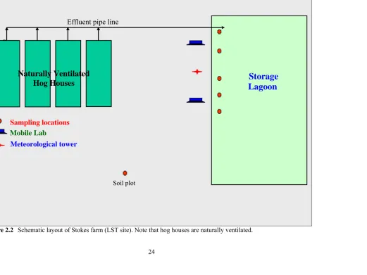
Figure 2.2 Schematic layout of Stokes farm (LST site)………...…...24

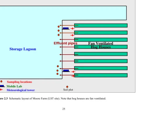
Figure 2.3 Schematic layout of Moore Farm (LST site)……….…………...…...25

Figure 2.4 Schematic layout of Barham Farm (potential EST)………...26

Figure 2.5 Schematic layout of Constructed Wetlands/Solid Separator Technology (potential EST).……….…...27

Figure 2.6 Schematic of the dynamic flow-through chamber system .……….…...28

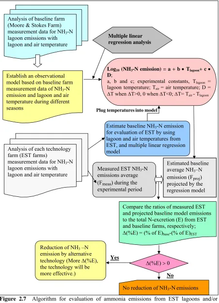
Figure 2.7 Algorithm for evaluation of ammonia emissions from EST lagoons and/or storage ponds...29

Figure 3.1a Site meteorological data during the 1st _{Stokes Farm measurement} period……….………..66

Figure 3.1b Site meteorological data during the 2nd Stokes Farm measurement period………...……..67

Figure 3.2a Site meteorological data during the 1st Moore Farm measurement period………...68

Figure 3.2b Site meteorological data during the 2nd Moore Farm measurement period………...69

Figure 3.3b Site meteorological data during the 2nd Barham Farm measurement

period………...71

Figure 3.4a Site meteorological data during the 1st Howard Farm measurement

period………...72

Figure 3.4b Site meteorological data during the 2nd Howard Farm measurement

period………...73

Figure 3.5 Diurnal pattern of ammonia flux Barham Farm from the storage pond, overflow pond, and overall measurements for warm and

cold seasons...74

Figure 3.6 Diurnal pattern of ammonia flux at Howard Farm from the wetland cells, finishing pond, and overall measurements for warm and cold

seasons…...75

Figure 3.7 Diurnal pattern of ammonia flux at Stokes and Moore farms for

warm and cold season measurements………...……...76

Figure 3.8 Lagoon NH3-N flux from the baseline farms during 1st and 2nd

measurement periods for Stokes and Moore Farms…………...…...77

Figure 3.9 Lagoon NH3-N flux during 1st and 2nd measurement periods for

Barham Farm (EST), respectively…...…....…...…...78

Figure 3.10 Lagoon NH3-N flux during 1st (June 3-14; 2002) and 2nd (Dec. 2-13,

2002) measurement periods for Howard Farm (EST)………...79

Figure 3.11 Log (A flux/ton) versus difference between the air temperature and the lagoon temperature (∆T) at baseline farms for different ranges of

lagoon temperature...80 Figure 3.12 Seasonal variation of NH3-N emissions relative to the total nitrogen

1.0 BACKGROUND AND INTRODUCTION

Atmospheric ammonia (NH3) has a large influence on several environmental processes and therefore has several distinct fates within the atmosphere and in terrestrial and

aquatic ecosystems. NH3 reacts with acidic atmospheric species, such as sulfuric acid (H2SO4), nitric acid (HNO3), and hydrochloric acid (HCl), to form ammonium aerosols, namely ammonium bisulfate (NH4HSO4), ammonium sulfate ((NH4)2SO4), ammonium nitrate (NH4NO3), and ammonium chloride (NH4Cl). Approximately 10% of atmospheric NH3 also reacts with hydroxyl radicals (.OH) to form amide radicals (.NH2) (Finlayson Pitts and Pitts 2000; McCulloch et al., 1998). These reactions can be summarized as follows:

NH3(g) + H2SO4(l) → NH4HSO4(l) (1) NH3(g) + HNO3(g) ↔ NH4NO3(s) (2) NH3(g) + HCl(g) ↔ NH4Cl(s) (3) NH3(g) + H2O(l) → NH4+ + OH- (4) NH3 + .OH →.NH2 + H2O(l) (5) (Finlayson Pitts and Pitts, 2000).

NH3 undergoes wet and dry deposition to the surface, depositing close to its emission sources due to its relatively short residence time in the atmosphere of 1-5 days (Warneck

2000).This residence time increases when NH3 transforms into the ammonium ion (NH4+) in aerosol form. Particulate NH4+ remains in the atmosphere for a longer period of time (1-15 days) due to a decrease in dry deposition velocity (Aneja et al., 1998).Therefore, it travels

and deposits farther from its source and can affect ecosystems over larger spatial scales.

Some of the detrimental effects of high concentrations and depositions of reduced N

1) Respiratory disease caused by exposure to high concentrations of

photochemical and fine particulate matter

2) Nitrate contamination of drinking water

3) Eutrophication, harmful algal blooms and decreased surface water quality

4) Nitrogen saturation of forest soil

5) Soil acidification

Atmospheric deposition of nitrogen compounds contributes approximately 35-60% of

nitrogen loading in coastal waters (Whitall et al., 2003; Pearl, 1995). An excess of nitrogen in

coastal waters gives rise to environmental hazards such as toxic and non-toxic phytoplankton

blooms, fish kills, and general declines in fisheries (Paerl 1995). In North Carolina, nutrient

loading has influenced coastal river systems, such as the Neuse River Basin, for several years

(Aneja et al., 1998). Elevated nitrate (NO3-) concentrations have been also observed in the North Carolina Coastal Plain Region (Showers, 1997).

Domestic animal waste produces the largest fraction of global atmospheric NH3 emissions, contributing 20-35 Tg of nitrogen per year (Bouwman et al. 1997; Warneck 2000)

(Figure 1.1). Swine waste produces the largest amount of NH3 emissions in North Carolina, releasing an estimated 68,540 tons of nitrogen per year (Aneja et al., 1998). This amount

represents 47% of the total NH3 emissions for the state and accounts for approximately 21% of North Carolina’s nitrogen budget (Aneja et al., 2001) (Figure 1.2). Soils, fertilizers, and

biomass burning also release NH3 into the atmosphere.

The statewide hog population has increased to almost 10 million in the last several

decades (NCDA 1999) (Figure 1.3). In response to the extensive growth of the hog industry

previously imposed moratorium on the construction of new swine facilities and the expansion

of existing swine facilities until September 2007. The growth of North Carolina’s hog

industry has largely occurred in the Coastal Plain Region, where more than 8.5 million hogs

currently reside (Aneja et al., 2000) (Figure 1.4).

Under certain meteorological conditions, NH3 emissions from the Coastal Plain Region have enhanced the wet deposition of NH4+ and NH3 at National Atmospheric Deposition Program/National Trend Network (NADP/NTN) sites that lie up to 80 kilometers

away from NH3 sources (Walker et al., 2000). Many sensitive ecosystems lie within 80 kilometers of NH3 area sources in North Carolina. Ecosystems in proximity to high NH3 emission sources and NH3/NH4+ deposition are subject to potential environmental consequences, including aquatic eutrophication and soil acidification. Quantification of NH3 emission sources and development of emission factors are necessary in order to assess the

potential extent of such environmental effects. Such a task requires extensive field

measurements at confined animal feeding operations (CAFOs), i.e. swine waste agricultural

operations.

There are several factors that influence NH3 emissions from CAFOs (Griffing et al., 2003; Westerman et al., 2000):

• Nitrogen content of the feed

• Conversion factor between N in animal food and N in the meat and milk (amount of N

waste available)

• Animal age and/or weight

• Animal housing system

Recent studies, using a mass balance approach to estimate NH3 emission rates, found that hog houses represent a more significant source than previously thought (Doorn et al., 2002).

Based on a review of published swine data, Westerman et al. (2000) estimated the loss of

ammonia from barnhouses to be around 15% of total nitrogen excreted. Griffing et al. (2003)

used the mass balance method to estimate that about 80% of ammonia loss was due to

volatilization from liquid waste storage systems. For this study, the mass balance method was

employed to estimate NH3-N loss rates relative to the nitrogen waste available for conventional waste lagoon storage systems for comparison with alternative waste treatment

methods.

Program OPEN (Odor, Pathogens, and Emissions of Nitrogen) is an integrated study

of the emissions of ammonia, odor and odorants, and pathogens from potential

environmentally superior technologies (ESTs) for swine facilities. It is funded by the Animal

and Poultry Waste Management Center at North Carolina State University. Its main purpose

is to evaluate potential environmentally superior swine waste management technologies that

have been developed and implemented under an agreement between the North Carolina

Attorney General and several companies that own 10% of the swine farms in North Carolina,

mostly employing the conventional Lagoon and Spray Technology (LST). Under Program

OPEN, ESTs implemented at selected swine facilities are being evaluated to determine if

they would be able to substantially reduce atmospheric emissions of NH3, odor, and pathogens. This study focuses on the emissions of nitrogen in the form of ammonia (NH3-N 14/17) from different components/processes involved in waste handling and treatment,

including waste storage ponds, barnhouses, and spray fields at two selected EST farms and

farms. This study is also a continuation and extension of a Master’s Thesis research by

Heather Arkinson (2003) who analyzed the data collected at the two EST farms (Barham and

Howard) in April and June of 2002, both representing the warm season only.

The primary objective of this study was to quantitatively measure and estimate

ammonia fluxes from various swine waste storage ponds at two potential Environmentally

Superior Technologies (ESTs), by using a dynamic flow-through chamber system with an

environmentally controlled mobile laboratory, and to compare them with fluxes from two

conventional Lagoon and Spray Technology (LST) swine waste facilities. A special emphasis

is placed on quantifying the emissions of ammonia, using a mass balance method, to develop

emission factors based on nitrogen losses from major components of the swine waste

treatment systems from LSTs and ESTs and to investigate their seasonal variability. A

secondary objective was to analyze the measured NH3 fluxes with respect to changes in physiochemical parameters such as lagoon temperature, air temperature, pH, and total

ammoniacal nitrogen (TAN), and to obtain multiple regression relations for ammonia fluxes

Global Sources of Ammonia Emissions

0

5

10

15

20

25

30

35

Fo ssil Fuel Co mbustio n

So il B io genic Emissio ns

Do mestic A nimal

Waste

Human Excretio n

B io mass B urning

Seas and Oceans

Tg N

/y

r

Total NH

Em issions = 76 Tg N/yr

Estimated Global Sources of Tropospheric Ammonia

Total N Emissions

0.3 Tg N/Yr

Highway Mobile NO

24%

Biogenic NO

3%

Large Industrial Inc.

Electric NO

24%

Area & Non-Road Mobile NO

7%

Other Agricultural NH

21%

Swine NH

21%

0

2

4

6

8

10

12

Hog Population (millions)

1955

1965

1975

1985

1995

2005

North Carolina Registered Swine Waste Management Systems

• Conventional Swine Waste Treatment Lagoon

2.0 METHODS AND MATERIAL 2.1 Sampling Sites

Ammonia flux measurements were conducted during two different seasons at four

swine facilities in eastern North Carolina. The two conventional Lagoon and Spray

Technology (LST) sites employed anaerobic lagoons, which did not require dissolved oxygen

in the bacteria treatment of organic wastes in the lagoons. These LST sites are also referred

to as “baseline” sites for comparison with EST sites. The two Environmentally Superior

Technology (EST) sites were Barham and Howard farms, which employed the In-ground

Ambient Digester Technology and Constructed Wetlands/Solid Separation Technology,

respectively. Locations of these farms in eastern North Carolina are shown in Figure 2.1.

Lagoon and Spray Field Technology

Sampling was conducted at Stokes Farm (35.43oN, 77.48oW, 17 m MSL), located near Trenton, NC in Pitt County, during September 9-20, 2002 and January 6-17, 2003. Four

naturally ventilated finishing barns housed 4,391 animals with an average weight of 104 kg

in the fall season and 3,726 animals with an average weight of 88 kg in the winter season.

Waste from the hog barns were flushed with recycled lagoon water and discharged into a

storage pond from a single effluent pipe. Lagoon surface flux measurements were taken from

various sampling locations from the lagoon illustrated in Figure 2.2.

Sampling at Moore Farm (35.14oN, 77.47oW, 13 m MSL) located near Kinston, NC in Jones County, was conducted during September 30 October 11, 2002 and January 27

-February 7, 2003. Eight fan-ventilated finishing barns housed 7,617 animals with an average

weight of 52 kg in the fall season and 5,784 animals with an average weight of 67 kg in the

discharged into a storage pond from eight effluent pipes, one for each hog barn. Lagoon

surface flux measurements plots are illustrated in Figure 2.3.

Environmentally Superior Technologies

1. In-ground Ambient Anaerobic Digester Technology

Sampling occurred at Barham Farm (35.70oN, 78.32oW, 130 m MSL), located near Zebulon, NC in Johnston County, during April 1-12, 2002 and November 11-22, 2002. The

potential EST was an In-ground Ambient Digester Technology, which consisted of a covered

anaerobic waste lagoon system (Figure 2.4). The primary anaerobic waste treatment lagoon

was covered by an impermeable layer of 40 mm thick high-density polypropylene that

prevented gaseous methane and other gases from escaping into the atmosphere during this

digestion process. The trapped methane gas was extracted and burned in a biogas generator

that provided electricity for the greenhouses and powered a water heater used for farm

production activities. The effluent from this primary covered lagoon was discharged into a

secondary stage lagoon, referred to as a storage pond. Biofiltration devices pumped effluent

from the storage pond where bacteria oxidized the reduced forms of nitrogen from the

effluent to nitrate (NO3-). This nitrified effluent was then used to flush out the hog production facilities and excess effluent was channeled into the larger overflow pond. A heavy polymer

baffle separated the overflow and storage ponds. The overflow pond was used to store excess

rainwater and overspills from the storage pond. The overflow pond was also pumped into a

biofiltration system where the nitrates in the water were used to fertilize greenhouse tomatoes

on the farm. Barham Farm was a farrow-to-wean operation, which included sows, gilts,

boars, and piglet up to three weeks old. Four gestation barns housed 3,360 sows and two

any given time. These figures were the same for both spring and winter measurement

periods. This study conducted ammonia flux measurements from the surfaces of the storage

and overflow ponds.

2. Constructed Wetlands/Solid Separation Technology

From June 3-14 and December 2-13, 2002, sampling was conducted at Howard Farm

(34.84oN, 78.40oW, 5 m MSL) located near Richlands, NC, in Onslow County. The potential EST was a waste treatment system that utilized a wetland ecosystem to reduce ammonia

emissions from the surface of the wetland cells (Figure 2.5). A solid separator was used to

separate the solid from liquid waste. The solid portion was applied to crop fields as fertilizer

and was also used to operate a vermiculture farm. The liquid effluent was broken down by

microbes contained in the Cattail plant species through oxidation and reduction. At the end of

the wetland cell process, the treated effluent was discharged into a finishing pond, which was

used for spray field applications for adjacent croplands. Howard Farm was a finishing

operation, which consisted of four hog houses with 3,618 pigs weighing an average of 64 kg

in the summer season and 3,881 pigs weighing an average of 97 kg in the winter season. This

study included ammonia flux measurements from the inlet, midpoint and outlet cells of the

wetland system, from the finishing pond, and from the soil of adjacent cropland.

2.2 Ammonia Flux Measurement Dynamic Flow-Through Chamber System

A flow-through dynamic chamber system with a variable-speed continuous impeller

stirrer (Aneja et al., 2000; Chauhan 1999; Kim et al., 1994; Kaplan et al., 1988) was used to

in height (a volume equal to 24.34 L), was fitted into a circular hole cut into the center of a

1.2 by 1.2 meter floating plywood platform, which penetrated the lagoon surface by ~7 cm.

To create a closed system inside the chamber, a seal was formed between the bottom of the

cylinder and the lagoon water. The cylindrical chamber was lined with a 5-mm thick

fluorinated ethylene propylene (FEP) Teflon sheet throughout the inside surface of the

chamber. Compressed zero grade air, which was used as a carrier gas, was passed through the

chamber at a variable flow rate of 4-8 lpm using a mass flow controller. The air inside the

chamber was ideally well mixed by a variable-speed, motor driven Teflon impeller ranging

from speeds of 40-60 rpm for this study. Roelle (1996) found that varying the speed of

Teflon impeller did not produce any significant changes in the calculated NO soil flux using

the chamber method. Research conducted on pressure differences between the outside

atmosphere and air within a chamber using a tilted water manometer indicated that pressure

differences were below detection limits (0.2mm H20) (Johansson and Granat, 1984). A vent line was fitted to the exiting sample line to prevent over pressurization and was bubble tested

periodically to check for under pressurization or leaks in the enclosed system. Sample lines

did not exceed 10 meters. Bunton (1999) conducted an experiment to explore possible

differences between air temperature inside the chamber and the ambient temperature. The

study found maximum temperature differences of 2.5oC and 3.4oC over two twenty-four hour experiments, which may have minimal effect on the temperature of the lagoon inside the

chamber.

The sample exiting the chamber traveled through Teflon tubing (6.35 mm outside

diameter, 3.97 mm inside diameter) to the ammonia detection instruments. The entire closed

reactions with sample flow. For soil measurements, the chamber was placed on a stainless

steel ring which was inserted into the soil, one day prior to sampling. Soil flux measurements

were taken two hours after the insertion of the ring to ensure steady-state conditions in the

chamber. NH3 emission data were not collected during precipitation events. Temperature Controlled Mobile Laboratory

A temperature-controlled mobile laboratory housed all detection instrumentation for

this study. The mobile laboratory consisted of a modified Ford Aerostar van with a 13,500

BTU air conditioner unit. The temperature inside the van was regulated for effective

performance of the ammonia analyzers. A 110-volt outlet was used to power the air

conditioning and all detection instruments.

NH3 Detection Instrumentation

Once the dynamic flow-through chamber system reached steady-state conditions,

NH3 concentrations were measured using a Thermo Environmental Instruments (TEI) Model 17c chemiluminescence Ammonia Analyzer from the sample flow exiting the chamber. The

17c ammonia analyzer separated the incoming sample flow into three separate parts. The first

path mixed the sample flow with ozone (O3) and all of the nitric oxide (NO) within the sample reacts to produce a reading of NO concentration via the standard chemiluminescence

technique. The second path involved the sample flow passing through a molybdenum

converter (325oC), which converts all oxidized forms of nitrogen (NOx) to NO. This sample then reacts with O3 in order to quantify the concentration of NOx. The third path flows through a stainless steel converter (775o_{C) where both NO}

oxides of nitrogen (NOx) (TEI, 2000). The following chemical reactions and other relations summarize the TEI 17c Ammonia Analyzer chemiluminescence technique for the TEI Model

17c Ammonia Analyzer:

NO + O3 Æ NO2* + O2 (6)

NO2* Æ NO2 + hν (7)

NT = NOx + NH3 (8)

NT – NOx = NH3 (9)

Calibrations for the TEI Model 17c Ammonia Analyzer were conducted using a TEI

Model 146 dilution-titration instrument in conjunction with cylinders of 20 ppmV and 900

ppmV of NH3 in N2 and zero grade air (Machine and Welding Purity Gases, NIST certified). The TEI 146 was serviced and calibrated to specification by the manufacturer and was

re-certified by North Carolina Division of Air Quality (NCDAQ) technicians. A multipoint

calibration was conducted before each two-week field measurement campaign. Zero and span

checks were conducted every day of the experiment according to the TEI 17c Ammonia

Analyzer Operator’s Manual (TEI, 2000).

2.3 Automated Data Collection

A Gateway laptop computer and a Campbell Scientific CR21X Datalogger (PC208W

software) were used as an automated data acquisition system. The CR21X datalogger

recorded 15-minute averaged measurements for NH3 concentrations inside the chamber, lagoon pH, and lagoon temperature. From a 10 m tower, the CR21X also collected 15-minute

averaged measurements of ambient NH3 concentrations at 10 m and meteorological parameters including wind speed and direction, air temperature, relative humidity, and solar

ammonia flux during data analysis. Recorded values were checked against the front panel of

detection instruments to ensure accuracy. There were no significant discrepancies found

between datalogger stored values and instrument display readings for this study.

2.4 Meteorological Measurements

At each sampling site, a 10 m meteorological tower was erected to measure wind

speed and direction, air temperature, relative humidity, and solar radiation. All

meteorological instrumentation for this study were purchased from Campbell Scientific

Incorporated (CSI), Logan, Utah. A Met One Instruments Model 034B-L Windset was used

to measure wind speed and direction at 10 m above the surface. The Model 034B-L consists

of an integrated cup anemometer and a wind vane. Accuracy of the measured wind speed

component is ± 0.12 m/s for wind speeds below 10.1 m/s and ± 1.1 % of reading for wind

speeds above 10.1 m/s. The wind direction component has an accuracy of ± 4o and a threshold of 0.4 m/s. Air temperature and relative humidity (RH) measurements were made

at 2 m height facing north with a Model HMP45C temperature and relative humidity probe

housed in a radiation shield. RH accuracy is ± 2% (0-90% RH) and ± 3% (90-100% RH)

while air temperature accuracy is 0.2-0.5oC. Solar radiation measurements were also made at 2 m height but facing south using a Model LI200X Silicon Pyranometer probe. Solar

radiation has an absolute error in natural daylight of 5% maximum and 3% typical. (CSI

Operator Manual Reference)

2.5 Lagoon Parameters and Ambient NH3

A CSI Model 11-L50 Innovative Sensors pH probe continuously monitored lagoon

Differences in lagoon temperatures inside and outside the chamber were found to be

insignificant (less than 1oC). These pH and temperature probes were submerged in the lagoon at a depth of 15~20 cm. Lagoon water samples were collected daily from measurement sites

and submitted to the Department of Biological and Agricultural Engineering (BAE), North

Carolina State University, for analysis of TAN (NH3-N + NH4+-N) measurements. The BAE Environmental Analysis Laboratory used an ammonia-salicylate method for automated

analysis of TAN.

Ambient NH3 concentrations were measured from Teflon tubing extending from the top of a 10 m meteorological tower to a TEI Model 17c Ammonia Analyzer housed in the

mobile laboratory unit. To prevent particles from entering into the sample inlet of the Model

17c Ammonia Analyzer, a one-stage Teflon filter (42 mm thick with 1 µm pore size) was

placed at the sample inlet at 10 m height.

2.6 Sampling Scheme

The dynamic flow-through chamber system was flushed with compressed air for an

hour, before a daily sampling period, to prevent accumulation of excess ammonia or moisture

in the chamber and sample lines in order to account for variability in different areas or

sections of each site’s lagoon storage system. The whole floating chamber system, the mobile

laboratory and meteorological tower, were moved one or two times to different sectors of the

lagoons in order to examine possible variability. The floating chamber itself was periodically

moved within a radius of 2 m from the previous plot on a daily basis.

2.7 Ammonia Flux Calculation

In order to calculate ammonia flux for this study, the following mass balance equation

[ ]

_{[ ]}

C

V

q

V

LA

V

JA

V

C

q

dt

dC

⎟

⎠

⎞

⎜

⎝

⎛

₊

−

⎟

⎠

⎞

⎜

⎝

⎛

₊

=

where C NH3 concentration in the chamber (ppbV) Cair NH3 concentration in ambient air (ppbV)

q flow rate of compressed air through the chamber (lpm)

V volume of the chamber (24.34 L)

A surface area covered by chamber (m2)

Aw inner surface area of the chamber of inner and upper wall surfaces (0.374 and 0.209 m2 respectively)

L total loss of NH3 in the chamber per unit area (m min-1) due to reaction with inner and upper walls of the chamber

h internal height of the chamber (45.7 cm)

J emission flux per unit area (µg NH3-N m-2 s-1)

Zero air was used as a carrier gas, so Cair is assumed to be zero. Since the chamber is

assumed to be well-mixed, concentration, C, is constant within the chamber. At steady-state

conditions, the change of concentration with respect to time will be zero. Equation (1) can be

simplified as: eq

C

V

q

V

LAw

h

J

⎟

⎠

⎞

⎜

⎝

⎛

₊

=

Loss term (L) was determined experimentally while equilibrium-state ammonia (Ceq),

flow rate (q) and dimensions of the chamber (V and h) were all measured. Kaplan et al.

⎥⎦

⎤

⎢⎣

⎡

−

−

−

C

C

t

C

C

(

)

ln

state NH3 concentration measured by the chamber system at a constant flow rate (12-14 lpm). Ceq is the measured NH3 concentration at a second equilibrium state at a reduced flow rate (4-6 lpm) into the chamber system. C(t) depicted NH3 concentration at any time, t, during the transition between the first and second equilibrium states. The following equation shows how

L is determined:

⎟ ⎠ ⎞ ⎜ ⎝ ⎛ ⎟ ⎠ ⎞ ⎜ ⎝ ⎛ ₋ = w A V V q line of slope

L (12)

where A equals the area of the inner walls of the chamber.

2.8 Climatological Data

Climatological data provided by the State Climate Office of North Carolina, located

at North Carolina State University, were used to compare monthly averages of air

temperature and precipitation for the experimental period month against the monthly

averaged 10-year average data for the same month. Historical climate data revealed normal

or abnormal variations of air temperature and precipitation parameters during the field

experimental periods. Significant climatological variations from 10-year averages for the

months of the experimental periods can be used to identify abnormal meteorological

conditions that might suggest atypical data obtained from an EST or LST site which may not

be representative of that particular month or season.

Hog feed analysis was used to calculate the mass of nitrogen excretion produced from

each experimental site. Based on hog feed, weight and population, the following equation

was used to determine the amount of nitrogen excretion for each farm:

1000

)

1

(

%

×

−

×

×

=

W

ER

N

F

E

where E Nitrogen Excretion (kg N/1000 kg LAW/ year)

where LAW = Live Animal Weight

F Feed consumed (kg/pig/year)

%N percentage of nitrogen in feed, expressed as a fraction

ER Feed efficiency rate (PigCHAMP, 1999) depending on farm operation type (e.g. wean to

farrow, feeder to finish)

W Average weight of hog for each farm (kg)

Nitrogen excretion data were used to determine the total nitrogen introduced into a swine

CAFO and for normalizing the NH3-N emissions from its individual components (barns, lagoon, etc.).

2.10 Baseline Observational Statistical Model

In order to evaluate the potential reduction of total nitrogen based on animal feed for

ESTs (Barham and Howard farms), Stokes and Moore farms were chosen as baseline farms

(LSTs) for obtaining background measurements of ammonia. These LST sites were used to

compare the effectiveness of EST sites in reducing nitrogen based on the ratio of total

nitrogen emissions from the liquid waste storage system and the total nitrogen excretion

based on animal feed analysis. This ratio is denoted as %E and is estimated from the

100 ) ( ) ( % _⎥× ⎦ ⎤ ⎢ ⎣ ⎡ = excreted N total Feed Animal on based Excretion Nitrogen emitted N Lagoons from Emissions Nitrogen Total

E (14)

Experimental periods for ESTs were chosen at different times of the year, therefore

environmental conditions were different at each site. In order to account for these

differences, a multiple regression analysis of the dependence of ammonia emission on

measured environmental parameters at the two baseline sites was conducted. Figure 2.7

depicts the algorithm employed to evaluate ESTs with lagoon and/or storage ponds based on

the strong multiple linear regression relationship between NH3 flux and lagoon temperature and the difference between air and lagoon temperature. First, data analysis of NH3-N measurements from baseline farms (Stokes and Moore farms) and the corresponding air and

lagoon temperatures were performed to obtain the observational statistical model relationship

based on multiple linear regression analysis as shown below:

) * ( ) ( ) / * (

10 Area Ammonia Flux ton a b T c T

Log = + ∗ lagoon + ∆ (15)

where a, b and c are experimental constants, Tlagoon represents lagoon temperature, Tair

represents air temperature, ∆T = Tair - Tlagoon. Area denotes the surface area of the lagoon at

the baseline farm where flux was measured and ton represents the total live animal weight at

the farm in metric tons (1000 kg). When ∆T was found to be positive or ∆T>0, then (c*∆T)

was used in the equation but when ∆T was negative or ∆T<0, then (c*∆T) was zero. The

reasoning for employing ∆T in the statistical model will be discussed in later sections. By

inserting averaged measurements of lagoon temperature and ∆T (only when Tair > Tlagoon) for the experimental period and appropriate constants/coefficients of the observational model, an

experimental period. This comparison was performed by calculating the ratios Fmeasured/total N excreted from the EST sites and Fprojected//total N excreted from baseline farms. The potential reduction of normalized NH3-N emission from EST sites was determined from the following equation:

ESTs of E baselines of

E

E) % %

(% = −

∆ (16)

where positive ∆(%E) would show that an EST is effective in reducing NH3-N relative to the total N excreted while a negative ∆(%E) would show no NH3-N reduction from an EST site. An important assumption for the potential reduction of nitrogen emission from EST sites is

that the total N excretion for baseline farms should be fairly constant throughout the year as

is shown in the results of this study. Hog weight, hog population, %N of hog feed, and hog

feed efficiency rates (ER) based on age are all considered in the evaluation of EST sites using

the observational statistical model.

2.11 Measurement Error Calculations

In order to determine confidence intervals for the calculation of overall %E, from the

baseline statistical model and during the EST experimental periods, conservative

measurement errors were assigned to nitrogen excretion, lagoon emission, and barn emission

values. Standard error estimates for calculated nitrogen excretion values for EST and LST

sites were 10%. The average NH3-N baseline flux value from the statistical model, Fprojected, and the measured averaged NH3-N flux value, Fmeasured, during the actual EST experimental period were estimated to have standard errors of 20%. The standard error that was assigned

to barn emissions (OP-FTIR method) conducted by Dr. Lori Todd’s ammonia group, from

Figure 2.1 Experimental research site locations in eastern North Carolina

Howard Farm Richlands, NC

Onslow County

Lagoon and Spray Technology (LST)

Environmentally Superior Technology (EST)

Barham Farm

Stokes Farm Zebulon, NC

Scuffleton, NC

Johnston County

Pitt County

Moore Farm Trenton, NC

Effluent pipe line

Storage

Lagoon

Naturally Ventilated

Hog Houses

Sampling locations

Mobile Lab

Meteorological tower

Storage Lagoon

Effluent pipes

Fan Ventilated

Hog Houses

Sampling locations Mobile Lab

Soil plot

Storage

Figure 2.4 Schematic layout of Barham Farm which employed the Covered In-Ground Ambient Anaerobic Digester

Technology (potential EST).

Greenhouses

Covered

Lagoon

Overflow

Pond

Pond

Nitrification Nitrification

Waste effluent flow

Sampling Locations

Biofilter Pit Flush

Biofilter

Mobile Laboratory

Fan Ventilated

Hog Houses

Figure 2.5 Schematic layout of Howard Farm which employed the Constructed Wetlands/Solid Separator Technology (potential

Solid Separator

312 140

108 80

90

4

Power

Fan Ventilated

Hog Houses

Storage Manholes

Finishing Pond

Inner Cell

Outer Cell

Wheat field

24

_{Waste In}

Waste In

_{Waste Out}

Mobile Laboratory

Generator

Sampling Locations

Figure 2.6 Schematic of the dynamic flow-through chamber system. The chamber fits inside a wooden floatation device,

Outflow

Flow Controller

Inflow

Wooden Floating

Platform

Lagoon

Continuous

Duty Motor

Impeller Stirrer

Zero Air

(no NH

or NO

)

Mobile

Laboratory

Van

Meteorological Tower

Vent Line

pH Probe

Temperature Probe #1

Figure 2.7 Algorithm for evaluation of ammonia emissions from EST lagoons and/or Analysis of baseline farm

(Moore & Stokes Farm) measurement data for NH3-N lagoon emissions with lagoon and air temperature

Establish an observational model based on baseline farm measurement data of NH3-N emission and lagoon and air temperature during different seasons

Log10 (NH3-N emission) = a + b • Tlagoon+ c • D;

a, b and c; experimental constants, Tlagoon =

lagoon temperature; Tair = air temperature; D = ∆T when ∆T>0, 0 when ∆T<0; ∆T= Tair - Tlagoon

Analysis of each technology farm (EST farms)

measurement data for NH3-N lagoon emissions with lagoon and air temperature

Estimate baseline NH3-N emission for evaluation of EST by using lagoon and air temperatures from EST, and multiple linear regression model

Plug temperaturesinto model

Measured EST NH3-N emissions average (Fmeas) during the experimental period

Estimated baseline average NH3–N emission (Fproj) projected by the regression model

Compare the ratios of measured EST and projected baseline model emissions to the total N-excretion (E) from EST and baseline farms, respectively;

∆(%E) = (% of E)base-(% of E)EST

No reduction of NH3-Nemissions

No Yes

Reduction of NH3 –N emission by alternative technology (More ∆(%E), the technology will be more effective.)

Multiple linear regression analysis

3.0 RESULTS AND DISCUSSION 3.1 Climatological Data Analysis

Based on analysis of precipitation and temperature over a 50 year period (1949-1998)

from 75 recording stations, precipitation in North Carolina has increased, especially during

the cooler seasons (Boyles and Raman, 2003). Although that study did not include any data

after 1998, individual analyses generally show that the last decade was the warmest and

wettest in the later half of the last century. Other statewide general patterns, over the 50 year

period analysis, include decreased precipitation during the summer and a decreasing trend

between the difference of maximum and minimum temperatures possibly due to increased

cloud cover and precipitation (Boyles and Raman, 2003; Dai et al., 1999; Easterling et al.,

1997). Note that statewide climate patterns do not always reflect long term climate trends for

individual recording stations.

EST sites

Climatological analysis of precipitation and air temperature trends were performed to

compare monthly 10-year averages (1992-2001) with monthly averages during which

measurements were conducted. By performing this analysis, abnormal meteorological

conditions based on precipitation and air temperature difference may help to explain atypical

data obtained during the experimental periods. Table 3.1 summarizes the climatological

findings from this analysis for ESTs and LSTs. Climatological data were obtained from the

State Climate Office (SCO) of North Carolina ECONET and National Weather Service

Cooperative Observer Network (NWS/CON) recording stations.

Barham Farm climatological data were obtained from the Clayton station for the

precipitation from 1992-2001 for the month of April was 7.3 cm and 4.1 cm for the month of

April 2002. For the month of November, the 10-year monthly averaged precipitation

(1992-2001) was 8.3 cm and 9.0 cm for November 2002. For the 10-year monthly averaged air

temperature for the month of April from 1992-2001, air temperature was 15.4oC and 17.3oC for the month of April 2002. For the November 2002 campaign, the 10-year monthly

averaged air temperature was 11.0oC and 9.3oC for November 2002.

For Howard farm, the Hoffman Forest station was used to obtain climatological

records for the June and December 2002 campaigns. The 10-year monthly averaged

precipitation from 1992-2001 for the month of June was 15.2 cm and 9.4 cm for June 2002.

For the month of December, the 10-year precipitation data was 7.9 cm and 7.6 cm for

December 2002. The 10-year air temperature data was 24.4o_{C for June and 24.6}o_{C for June} 2002. For December, the 10-year air temperature data was 8.8oC and 9.3oC for December 2002.

The spring campaign for Barham Farm showed a decrease of precipitation of 4.1 cm

compared to 10-year precipitation records for the months of April 1992-2001. With a higher

monthly air temperature average of 17.3o_{C for April 2002 compared to 15.4}o_{C for April} 1992-2001. It may be inferred that ammonia flux measurements were taken during atypically

warmer and drier conditions. It is possible that the warmer and drier atmospheric conditions

during the April 2002 campaign would positively influence ammonia fluxes for Barham due

to a potential increase of lagoon temperatures. For Howard farm, air temperature data for

long term and current records were almost identical at 24.5o_{C for the June 2002 measurement} period, but precipitation was lower during the same experimental period at 9.4 cm compared

December 2002 campaign, only minor differences were noted in precipitation data but the

average air temperature for December 2002 was slightly higher compared to the 10-year

average for the same month from 1992-2001.

LST sites

Stokes Farm climatological data were obtained from the Greenville station for the

September 2002 and January 2003 measurement campaigns. The 10-year monthly averaged

precipitation from 1992-2001 for the month of September was 18.5 cm and 11.9 cm for the

month of April 2002. For the month of January, the 10-year monthly averaged precipitation

(1992-2001) was 12.2 cm and 18.3 cm for January 2003. For the 10-year monthly averaged

air temperature for the month of September from 1992-2001, air temperature was 22.4oC and 24.2oC for the month of September 2002. For the month of January, the 10-year monthly averaged air temperature was 6.3oC and 6.9oC for January 2003.

For Moore farm, the Kinston station was used to obtain climatological records for the

October 2002 and January-February 2003 campaigns. The 10-year monthly averaged

precipitation from 1992-2001 for the month of October was 9.0 cm and 6.6 cm for October

2002. For the months of January-February, the 10-year precipitation data were 11.4-7.4 cm

and 8.4-9.4 cm for January-February 2003, respectively. The 10-year air temperature data

was 16.1oC for October (1992-2001) and 18.6oC for October 2002. For January-February, the 10-year air temperature data were 6.1-7.4oC and 5.5-7.2oC for January-February 2003. Climatological analysis conducted for LST experimental periods showed some

deviation from 10 year averages for precipitation and little deviation in air temperature

parameters. Stokes Farm experienced generally drier conditions during the fall season

Air temperature data did not show abnormal patterns for both fall and winter season research

periods at Stokes farm. A similar climatological trend is observed for Moore Farm where fall

season measurement periods were generally drier and winter measurement periods were

wetter but no significant differences can be seen in air temperature data for both seasons.

3.2 Site Meteorological Data

Means and standard deviations of meteorological measurements are summarized for

all farms in Table 3.2. Wind speed averages and standard deviations for spring and fall

seasons at Barham Farm were similar at 1.9 ± 0.9 m/s and 1.5 ± 1.1 m/s, respectively.

Compared to Barham Farm, Howard Farm had somewhat higher wind speed averages and

standard deviations of 2.2 ± 1.4 m/s for the summer and 2.4 ± 1.5 m/s for the winter sampling

period. During the early fall season, Stokes Farm exhibited similar wind speeds and standard

deviations, as that of Howard Farm during the summer and Barham Farm during the spring,

at 2.0 ± 1.5 m/s, while winter measurements were highest for all experimental sites at 3.3 ±

2.3 m/s. Moore Farm had wind speed measurements of 1.5 ± 1.1 for the October 2002

experimental period, which was identical to Barham Farm measurements during the

November 2002 experimental period, and higher measurements, during the winter

measurement period, of 2.3 ± 1.7 m/s.

Wind directions for the spring season sampling period at Barham Farm were 180 ±

120 degrees or generally from the south, but with large variability in wind directions

originating from the southeast and southwest. In the fall season, measurements of wind

direction at Barham farm were 266 ± 75 degrees, or predominantly from the west. A similar

trend is observed at Howard Farm, during summer season measurements, where wind

from the east and south directions, and during the winter measurement period measured wind

directions were from 252 ± 100 degrees or from the southwest to west. At Stokes Farm, wind

directions were 143 ± 95 degrees or mainly from the southeast direction with significant

variations during the fall measurement period. During the winter sampling period at Stokes

Farm, wind directions were 232 ± 41 degrees or mainly from the southwest with small

variability. Wind direction measurements were from 142 ± 87 degrees or mainly from the

southeast for the fall measurement period at Moore Farm, which was almost identical to fall

measurements at Stokes Farm, and measurements during the winter season were from 277 ±

93 degrees or generally from the west. Warm season measurements of wind directions

seemed to generally come from the south to southeast directions, while cooler season

measurements were mostly from the southwest to west directions.

Air temperature measurements were 14.8 ± 4.4oC for the spring field measurement campaign and 10.3 ± 5.3oC for the fall measurement period at Barham Farm. At Howard Farm, air temperature averages and standard deviations were 23.3 ± 5.2oC for the summer experimental period, and during the winter experimental period, air temperatures were 4.2 ±

4.3o_{C. Air temperature measurements at Stokes Farm were 24.1 ± 4.1}o_{C during the early fall} measurement period and 4.6 ± 5.8oC during the winter season, which were comparable with Howard Farm measurements for both warm and cold seasons. Averages and standard

deviations for Moore Farm were 23.5 ± 4.4oC and 6.8 ± 5.5oC for the fall and winter experimental periods, respectively. Moore Farm also showed similar air temperature

measurements with Stokes and Howard farms for warm and cold seasons. For this study,

summer and early fall measurement campaigns had air temperature averages between

Hourly averaged wind speed, wind direction and air temperature were measured from a 10 m

tower, and their overall (composite) averages and standard deviations as functions of time of

day for each sampling period are illustrated in Figures 3.1-3.4 for all LST and EST sites.

Figures 3.1a and 3.1b represent such composite meteorological measurements from Stokes

Farm for fall and winter measurement periods, respectively. At Stokes farm, composite

hourly averaged wind speeds ranged from 0.8 to 3.7 m/s with highest wind speeds and

standard deviations during the early afternoon hours and lower wind speeds and standard

deviations during the early morning hours during the fall measurement campaign. Standard

deviations of hourly averaged wind direction measurements were fairly constant diurnally

and composite wind directions ranged from 111o to 201o during the same period. Composite hourly averaged air temperature data ranged from 19.3oC to 29.4oC and standard deviations were relatively small (~2-3oC) and did not vary significantly throughout the measurement period in the fall season. Winter season composite hourly averaged wind speeds, at Stokes

farm, ranged from 2.2 to 5.5 m/s with higher wind speeds and minimum standard deviations

in the mid-afternoon hours and lower wind speeds and maximum standard deviations during

the night. Average wind directions ranged from 213o _{to 251}o _{and did not vary significantly} throughout the winter experimental period, especially during the day. Composite hourly

averaged air temperatures ranged from 0.9oC to 9.8oC for the winter season measurement period at Stokes farm.

Figures 3.2a and 3.2b represent composite hourly averaged data from Moore Farm for

fall and winter experimental periods, respectively. During the fall season measurement

campaign, average wind speeds ranged from 0.7 to 2.5 m/s with minimum wind speeds

hours. Wind direction measurements showed high standard deviations during the fall

measurement period and their composite mean values ranged from 112o to 175o. Mean air temperatures ranged from 19.0oC to 29.6oC with slightly higher standard deviations from hourly air temperature means from the late morning to late afternoon hours. Composite mean

wind speeds for winter season measurements at Moore ranged from 1.5 to 3.7 m/s with

maximum wind speeds during the mid-afternoon hours and minimum wind speeds during the

night. Mean wind directions ranged from 257o to 304o with large standard deviations throughout the winter measurement period. Composite mean air temperature ranged from

3.2oC to 13.4oC and exhibited fairly constant standard deviations diurnally.

Figures 3.3a and 3.3b illustrate composite hourly averaged meteorological parameters

for Barham Farm during the spring and fall measurement periods, respectively. Composite

mean wind speeds ranged from 1.4 to 2.8 m/s, while wind direction measurements ranged

from 101o to 284o during the spring experimental period. For the same period, composite mean air temperatures ranged from 9.5oC to 19.1oC. Standard deviations for wind speed averages were higher during the night, while those for wind directions were large throughout

the diurnal period. Standard deviations for air temperature were higher during the mid-day to

late afternoon hours. Fall season values of composite mean wind speed ranged from 0.9 to

2.7 m/s and showed large standard deviations for all hours. Mean wind directions ranged

from 230o to 286o with lower standard deviations during the day. Air temperature data showed high standard deviations during the night and composite averages ranged from 6.7oC to 15.7o_C.

Composite hourly averaged wind speeds, wind directions, and air temperatures for

measurements, respectively. During the summer experimental period, mean wind speeds

ranged from 0.8 to 3.9 m/s and showed more deviations in the middle to late afternoon hours.

Wind direction measurements ranged from 105o to 230o and had higher standard deviations from midnight to the late morning hours. Air temperatures exhibited higher standard

deviations during the night and their composite mean values ranged from 17.8oC to 29.1oC. During the winter measurement campaign at Howard farm, mean wind speeds ranged from

1.5 to 3.8 m/s while wind directions ranged from 223o to 307o with a minimum standard deviation at noon. Composite mean air temperatures ranged from 1.7oC to 9.3oC and standard deviations were diurnally consistent.

3.3 Ammonia Emissions from Spray Fields

The In-ground Ambient Anaerobic Digester Technology employed at Barham farm,

during the April and November 2002 measurement periods, was measured for ammonia

emissions from a soil surface that was not used for agricultural spray fields. Howard farm,

which employed the Constructed Wetlands/Solid Separation Technology, had also not

received land application of treated lagoon spray during the June and December 2002

experimental periods. Ammonia concentrations for non-spray and spray fields at EST sites

were below the detectable limit of 2 ppb for 200 ppb range (TEI, 2000). The same results

were found for the baseline sites at Stokes and Moore farms where soil flux measurements

did not coincide with land application of lagoon spray due to scheduling conflicts.

For mass balance considerations, soil measurements of ammonia from soils on

adjacent cropland should be considered for determining emission factors for subsystems of

swine operations for various seasonal conditions (National Research Council Report, 2003).

thirty-two times more ammonia than soils that were unfertilized. Although both lagoon effluent and

cropland soils contribute significant amounts of ammonia to the atmosphere, this study did

not find reportable data on soil emissions of ammonia for the summer, spring, fall and winter

measurement campaigns. Future measurements of ammonia emissions, from spray fields

used at swine farms, should coincide with times of lagoon spray from waste treatment

systems to establish a relationship between them.

3.4 Lagoon and Environmental Parameters

Means and standard deviations of NH3-N flux measurements and lagoon parameters are summarized for all farms in Table 3.3. For the April 2002 measurement campaign,

Barham Farm had average ammonia fluxes of 1,102 ± 640 µg NH3-N/m2/min from the storage pond and 1,249 ± 175 µg NH3-N/m2/min from the overflow pond with an overall average flux of 1,169 ± 519 µg NH3-N/m2/min. For the November 2002 measurement campaign, average ammonia flux measurements were 436 ± 39 and 234 ± 34 µg NH3 -N/m2/min for the storage and overflow ponds, respectively, with overall average ammonia flux of 352 ± 27 µg NH3-N/m2/min. Figure 3.5 illustrates hourly averaged ammonia flux measurements from storage and overflowing ponds, and compares overall measurements of

hourly averaged ammonia fluxes for warm and cold seasons. In the warm season, ammonia

flux measurements from the storage pond were higher than overflow pond measurements

during the day and lower during the night. Non steady-state operation of the EST may

explain higher average ammonia fluxes in the overflow pond during the warm season

sampling period at Barham Farm. During the cold season, the treated effluent in the overflow

pond exhibited consistently lower values of ammonia flux compared to storage pond