Parallel Processing Models For Image Processing Problems

VOT 72179

PARALLEL PROCESSING MODELS FOR IMAGE PROCESSING PROBLEMS

SHAHARUDDIN SALLEH BAHROM SANUGI

JABATAN MATEMATIK FAKULTI SAINS

UNIVERSITI TEKNOLOGI MALAYSIA

DEDICATION AND ACKNOWLEDGEMENT

ABSTRACT

ABSTRAK

TABLE OF CONTENTS

COVER i

DEDICATION AND ACKNOWLEDGEMENTS ii

ABSTRACT iii ABSTRAK iv

TABLE OF CONTENTS v

LIST OF FIGURES viii

LIST OF TABLES x

SYMBOLS AND NOTATIONS xi

CH. SUBJECT PAGE

1. RESEARCH FRAMEWORK

1.1 Introduction 1

1.2 Problem Statement 2

1.3 Objectives of Research 4

1.4 Scope of the Study 4

1.5 Report Outline 4

2. RECONFIGURABLE MESH COMPUTING NETWORKS

2.1 Introduction 6

2.2 Why do we need a parallel computer? 8

2.4 Memory computational models 15

2.5 Processor organization/topology 17

2.6 Reconfigurable mesh network (Rmesh) 18

2.7 Sorting algorithm example on Rmesh 23

3. DYNAMIC MULTIPROCESSOR SCHEDULING ON RMESH

3.1 Introduction 26

3.2 Dynamic task scheduling problem 28

3.3 Reconfigurable mesh computing model 31

3.4 Simulation and analysis of results 36

3.5 Summary and conclusion 39

4. RMESH MODEL FOR THE EDGE DETECTION PROBLEM

4.1 Introduction 40

4.2 Edge detection problem 41

4.3 Reconfigurable mesh computing model 43

4.4 RM model for detecting the edges 44

4.5 Summary and conclusion 46

5. SINGLE-ROW ROUTING USING ESSR

5.1 Introduction 47

5.2 Problem background 48

5.3 Review of state of the art 57

5.4 Enhanced simulated annealing approach 60

5.5 Experimental results and analysis 68

5.6 Summary and conclusion 70

6.2 Problem formulation 73 6.3 Complete graph partitioning strategy 74 6.4 Application of the frequency assignment problem 82

6.5 Summay and conclusion 83

7. SUMMARY AND FUTURE WORK

7.1 Summary of results 84

7.2 Open issues and proposal for future work 86

APPENDIX 88 REFERENCES 89

LIST OF FIGURES

Page

Figure 2.1: a conventional processor 10

Figure 2.2: A pipelined processor 11

Figure 2.3: SISD Model 12

Figure 2.4: SIMD Model 14

Figure 2.5: MIMD Model 14

Figure 2.6: The RAM model of sequential computation 15 Figure 2.7: The PRAM model of parallel computation 16 Figure 2.8: 2-dimensional RMesh with 16 processing elements 19

Figure 2.9: Torus 20

Figure 2.10: Four external ports for a node in a 2-dimensional RMesh network 20

Figure 2.11a: 2D mesh with fixed connection 22

Figure 2.11b : 2D reconfigurable mesh 22

Figure 2.13: A few patterns of the switch connection 23 Figure 2.14: Numbers in descending order from above 25

Figure 3.1: A reconfigurable mesh of size 4x 5 27

Fig.3.2: The m/m/c queueing model 30

Fig.3.3: A 4x 4 reconfigurable mesh network with two subbuses 33

Fig.3.4: Sample run from DSRM 37

Fig. 4.1: A 4 x 4 reconfigurable mesh network with two subbuses 43 Fig. 5.1: Net ordering L={N₁,N₃,N₂,N₅,N₄} with the reference line 51

Fig. 5.2: Realization from the ordering L={N1,N3,N2,N5,N4} 54 Fig. 5.3(a): Final net ordering based on virtual tracks 58

Fig. 5.3(b): Final realization with Q=2 and D=5 59

Fig. 5.4(a): Classification according to zones 60

Fig. 5.4(b): Final realization with Q=2 and D=6 60

Page

Fig. 5.6: ESSR flowchart 65

Fig. 5.7: Comparison between ESSR and SRR-7 67

Fig. 5.8: Final net realization of Example 1 using ESSR 67 Fig. 5.9: Energy against the number of doglegs in ESSR by pivoting Q 69

Fig. 6.1: Formation of nets based on the zones and levels in S₅ from C₅ 76 Fig. 6.2: Nets ordering with minimum energy, E =11, of C₅ using ESSR 80

LIST OF TABLES

Page

Table 2.1: Numbers to sort 24

Table 3.1: Sample run of 209 successful randomly generated tasks on 16 PEs 38

Table 5.1: Classification of nets in Example 1 58

Table 5.2: Comparison of experimental results 68

Table 6.1: Formation of nets in S5 from C5 79

SYMBOLS AND NOTATIONS

G a graph

m

C a complete graph with m vertices

m

S single-row representation of C_m Q congestion of the nets in S_m

D number of interstreet crossings (doglegs) in S_m E total energy in S_m

L partial order of nets arranged from top to bottom in S_m

j

v vertex j in the graph

j

d degree of vertex j in the graph m number of vertices in the graph

i

t terminal i

k

b left terminal of net k

k

e right terminal of net k

k

n net k, given as nk =(bk,ek)

m i y

n ,, the ith net in level y in Sm m

i y

b _,, beginning (left) terminal of the ith net in level y in S_m

m i y

e ,, end (right) terminal of the ith net in level y in Sm m

y

w _, width of every net in level y in S_m

m y

r , number of nets in level y in Sm j

CHAPTER 1

RESEARCH FRAMEWORK

1.1 Introduction

Numerous problems in science and engineering today require fast algorithms for

implementations and executions on computers. These problems involve massive

computations arising from intensive mathematical calculations with double precisions

variables and large array sizes. The solutions require high degree of accuracy and

constant updates that really take up the maximum capability of the host computers. As a

result, single-processor computers based on the von Nerumann architecture seldom

satisfy all these requirements. Fast computing platforms with large storage area for

processing data in the form of parallel computing networks become the ultimate tools

In our research, we study various number-crunching problems, formulate them as

solutions in the form of parallel algorithms and then develop these ideas into their

visualization models. The problems of interest in our research include image processing

and routing. We develop the parallel algorithms for these problems and their solutions

in the form of user-friendly softwares.

1.2 Problem Statement

The problem in this study consists of the development of fast algorithms for highly

intractable engineering problems. Three main problems are studied, namely, task

scheduling for parallel computing networks, image processing and routing for the VLSI

design as some of the applications in task scheduling.

In the first problem, we study the task scheduling problem for the parallel

computing network. A task is defined as a unit of job in a computer program. Task

scheduling can be stated as the problem of mapping a set of tasks, T , onto a set of

processing elements, , in a network, with the main objective of completing all the

jobs at the most minimum time. In this work, we study the problem of scheduling

randomly generated tasks on a reconfigurable mesh network. A mesh network consists

of processors arranged in a rectangular array. Each processor in the network has

i

k

P

the processing capability and some storage area for the data. The intermediate processor

communicates with its four neighbors through its east, west, north and south ports.

In the second problem, we study several methods for detecting the edges of an

image. An image consists of a rectangular array of pixels, each with a varying degree of

intensity represented as colours and gray tone scale. The problem of edge detection can

be stated as searching a set of boundary pixels that separate the high and low

intensities of the given image, . Edge detection is one of the most fundamental

components in image analysis, as the method contributes in solving problems such as

object recognition, noise reduction, multiresolution analysis, image restoration and

image reconstruction. Since an image is normally rectangular in shape, the parallel

mesh computing network provides a good platform for its solution. Physically, mesh

network provides an ideal tool for solving the image processing problem as each of its

processor directly maps the pixels of the given image. ) , (i j b

) , (i j f

In addition, we also study the routing techniques for the very large scale integration (VLSI) design problem in the printed circuit board (PCB). In VLSI, two main problems arise in order to produce a highly compact and integrated design. The

first problem is the placement of millions of minute electronic components into the

small area of the chip. The second problem deals with the development of routes that

connect pairs of these components to allow them to communicate with each other. In

this work, we study and develop a model for the second problem based on the

1.3 Objectives of Research

The objectives of our research are as follows:

1. To promote fundamental research that integrates mathematics with its

applications, especially in areas of engineering and information technology.

2. To develop and promote parallel algorithms and solutions on highly interactive

combinatorial problems, and its simulation and visualization models.

3. To promote learning groups on various problems of this nature in the community.

4. To contribute the ideas to the interested parties in industries for further

collaboration.

1.4 Scope of the Study

Our study is confined to the development of simulation models for task scheduling,

edge detection in image processing and routing problems based on the mesh network.

The work extends to the development of algorithms and user-friendly computer

softwares based on the personal computer Microft Windows environment.

1.5 Report Outline

The report is organized into seven chapters. Chapter one is the research framework where the problems, objectives and scope of the work are described.

discuss the architecture of the reconfigurable mesh which has ports that can be configured dynamically according to the requirements of the program.

In Chapter three, we discuss the task scheduling problem on the reconfigurable mesh network. Task scheduling is a combinatorial optimization problem that is known to have large interacting degrees of freedom and is generally classified as NP-complete. Task scheduling is defined as the scheduling of tasks or modules of a program onto a set of autonomous processing elements (PEs) in a parallel network, so as to meet some performance objectives.

In Chapter four, we present the edge detection method which is an application of the task scheduling problem. Edge detection is a technique of getting a boundary line which holds the key to other image processing requirements, such as object recognition, image segmentation, and image analysis. We concentrate on the development of the second-order Laplacian convolution technique on the mesh network for this problem.

Chapter five discusses another application of task scheduling, namely, the single-row routing problem. In the single-single-row routing problem, we are given a set of n evenly spaced terminals (pins or vias) arranged horizontally from left to right in a single row called the node axis. The problem is to construct nets in the list from the given intervals according to the design requirements. In this chapter, a model called the Enhanced Simulated annealing for Single-row Routing (ESSR) is proposed to represent the solution to the problem.

In Chapter six, we formulate the concept of transforming a complete graph into its single-row representation. This idea is a significant contribution in the sense that it generalizes the single-row routing as an effective application from other applications. Through this technique, any problem that can be represented by a graph is reducible to its the single-row routing representation.

CHAPTER 2

RECONFIGURABLE MESH COMPUTING NETWORKS

2.1 INTRODUCTION

Observation, theory, and experimentation are basic action for classical science. All these will lead to a hypothesis. From that, scientists will develop a theory to explain the phenomenon and design a physical experiment to test the theory. Usually the results of the experiment require the scientists either to refine the theory or completely reject it. And the process will repeat again and again. All this experiments may be too expensive or time consuming. Some may be unethical or impossible to perform.

Contemporary science, then, is characterized by observation, theory,

experimentation and numerical simulation. Numerical simulation is an increasingly important tool for scientists. Many important problems are just too complex that solving them via numerical simulation requires extraordinarily computers. High speed

numerical simulation of a phenomenon. Instead of doing physical experiments, they can save time through effective simulations.

The followings are some of the several categories of complex problems (Levin 1989) that require massive numerical computations:

1. Quantum chemistry, statistical mechanics, and relativistic physics. 2. Cosmology and astrophysics.

3. Computational fluid dynamics and turbulence.

4. Biology, pharmacology, genome sequencing, genetic engineering, protein folding, enzyme activity and cell modeling.

5. Global weather and environmental modeling.

These entire problems can be solved by the fastest computer in the world which is built of numerous microprocessors. This com puter is also known as parallel

computer. In order to keep up to this high speed computing, studying parallel algorithms is a necessity today.

This chapter is divided into five sections. Section 2.1 is the introduction, while in Section 2.2, we discuss the importance of parallel computers. A good analogy is

presented to make the problem easier to understand. Section 2.3 in this chapter reviews the paradigms of parallel processing. From the Flynn’s taxonomy , the architecture of a parallel can be classified as SISD, SIMD, MISD, and MIMD. The next section discusses the memory models of computation which is divided into serial and parallel. In a serial computational model, the model is called random access machine (RAM), while in parallel, it is called parallel random access machine (PRAM). Section 2.5 presents the topology of the network, which is the way processors are organized. The last section is about the Reconfigurable Mesh network. We discuss the architecture of the

2.2 WHY DO WE NEED PARALLEL COMPUTERS?

The solution to a typical numerical problem in engineering today requires the use of several large size multi-dimensional arrays, multi-level loops and the thousands of lines of code, in a single program. As a result, the program needs to be written in a very systematic manner, with proper software engineering techniques and implementations. The burden of a single computer system is greatly reducing by distributing the load to the processors in the system. As a result, the individual processors are not too

overloaded and the same amount of work can be completed in a much faster time with a network of cooperating processors.

A computer, as described in Zomaya (1996), is a digital electronic device with either a sequential or parallel design. A sequential computer is a random access memory model (RAM) that contains one processing element (processor) and an attached main-memory unit in an architecture known as the von Neumann design. This digital machine reads and executes instructions and data sequentially using only one processor. In contrast, a parallel computer consists of a set of at least two computing elements, all of which are connected in a network so that each one of them will be able to communicate, and share resources and energy with others in performing a job. The parallel counterpart to the RAM model, called the parallel random access memory (PRAM), has a set of synchronous processors connected to a shared memory.

Kolmogorov’s Theorem (Kolmogorov, 1957): Any continuous function f(x1,x2,...,xn) of

n variables x1,x2,...,xn on on the interval In can be represented in the form

f x x x_n h_j g x_{ij i}

i n

j n

( , ,...,_{1 2} ) ( )

1 1

2 1

= 



 _

= =

+

∑

∑

where hj and gij’s are continuous functions of one variable. Furthermore, the gij’s are fixed, monotonic increasing functions that are not dependent on f(x1,x2,...,xn). This theorem provides a very useful development of parallel algorithms that relate a problem with its solution in implicit or explicit manner.

A good analogy we can use to describe how the serial and parallel computers work is in the construction of a house. If there is only one worker who will do all the entire job (bricklaying, plumbing, and installing wiring, etc) by himself, he is going to take a very long time to finish a house. All the tasks will be done one by one in a sequence and this is called the sequential approach which is very slow way. However, by splitting the tasks to several workers, the construction can be completed much faster. The workers can be assigned different and independent tasks simultaneously, and this contributes to faster completion.

Figure 2.1: a conventional processor

This reason has lead many computer designers to develop the solution for this problem. The slowness of the computer in executing a task are caused by the access to memory. When the data is fetched from the memory, all the processor’s functional unit that perform the computation must remain idle. After executing, the result must be sent to the memory and again, this will involve some extra overhead. Another problem arises when the processor needs to fetch more than one operand at the same time. While the first operand is fetched, the second operand must wait until the first has completed its job. A solution to this problem lies in a co-operative system called interleaved memory. Interleaved memory consists of a small number of separately accessible memory units. In this system, several units of memory can be accessed at the same time through separate channels. Data too can be fetched without having to wait for channels to clear first.

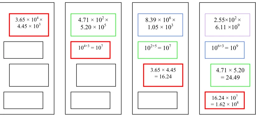
Another reason that causes the slowness in a computer is the tedious process of computations. Imagine a very large number to be multiply with another large number, of course, it will take a few small steps before the computation can be done. In a conventional computer, this step is done in a way which cause some processor idle while waiting for a task to be executed. A pipelined processor, as shown in Figure 2.2,

3.65 × 104 _× 4.45 × 103

104+3

3.65 × 4.45 = 16.24

can be used to solve this problem. It is effective for applications that require many repetitions of the same operation.

Figure 2.2: A pipelined processor

The same house construction anology can also apply in parallel computer. It seems like parallel when there are many workers doing different parts of the job. What makes the system is good is because each individual has several function unit. All the workers are differentiate by their speciality either in doing bricklaying, plumbing or wiring. This system is also said to have a coarse grain size because the tasks assigned to each worker are in certain amount. These people are similarwith processors in the parallel computer.

The laborers are communicated with each other. For example, bricklayers working next to each other must stay in close communication to make sure the build a uniform wall between section. This is called the nearest-network topology. However, such a system can lead to overhead because while sending the message to each other, the workers may talk a lot and do less job. That is why there must be another good

topology that can overcome this bottleneck. 3.65 × 104 _×

4.45 × 103

104+3 _{= 10}7

4.71 × 102 _×

5.20 × 105 8.39 × 10 6 _×

1.05 × 103

102+5 _{= 10}7

2.55×102 _×

6.11 ×109

106+3 _{= 10}9

4.71 × 5.20 = 24.49 3.65 × 4.45

= 16.24

2.3 PARALLEL PROCESSING PARADIGMS

Computers operate simply by executing a set of instructions on a given data. A stream of instructions inform the computer of what to do at each step. From the concepts of instruction stream and data stream, Flynn (Flynn, 1972) classified the architecture of a computer into four. Instruction stream is a sequence of instructions performed by a computer; a data stream is a sequence of data manipulated by an instruction stream. The four classes of computers are:

• Single instruction stream, single data stream (SISD)

• Single instruction stream, multiple data stream (SIMD)

• Multiple instruction stream, single data stream (MISD)

• Multiple instruction stream, multiple data stream (MIMD)

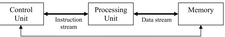
2.3.1 Single instruction stream, single data stream (SISD)

Most serial computers belong to the SISD class that have been designed based on the von Neumann architecture. In such computers, the instructions are executed

sequentially which means the computer executes one operation at a time. The algorithm used in this class is known as a sequential algorithm. Although a SISD computer may have multiple functional units, there are still under the direction of a single control unit. Figure 2.3 illustrates a SISD computer.

Figure 2.3: SISD

Data stream Instruction

stream

Control Unit

Processing

2.3.2 Single instruction stream, multiple data stream (SIMD)

SIMD machines consist of N processors, N memory, an interconnection network and a control unit. All the processor elements in the machine are supervised by the same control unit. These processors will be executing the same instruction at the same time but on different data. In terms of memory organization, these computers are classified as shared memory or local memory. To get an optimal performance, SIMD machines need a good algorithm to manipulate many data by sending instruction to all processors. Processor arrays fall into this category.

2.3.3 Multiple instruction stream, single data stream (MISD)

Among all four, MISD is the least popular model for building commercial parallel machine. Each processor in MISD machine has its own control unit and shares a common memory unit where data reside. Parallelism is realized by enabling each processor to perform a different operation on the same data at the same time. Systolic arrays are known to belong to this class of architectures. Systolic means a rhythmic contraction. A systolic array is a parallel computer that rhythmically ‘pumps’ data from processor to processor. The might be some changes in the data everytime it goes

Figure 2.4: SIMD Model

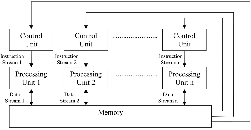
2.3.4 Multiple instruction stream, multiple data stream (MIMD)

MIMD machines are the most general and powerful system that implements the paradigm of parallel computing. In MIMD, there are N processors, N streams of instructions and N streams of data. As shown in Figure 2.5, each processor in MIMD has its own control unit.

Figure 2.5: MIMD Model

2.4 MEMORY COMPUTATIONAL MODELS

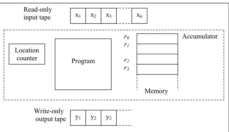
There are two models of computation. First is the serial model of computation while the other one is the parallel model of computation. The random access memory (RAM), as shown in Figure 2.6, is the sequential model of computation. The model consists of a memory, a read-only input tape, a write-only output tape, and a program.

.

Figure 2.6: The RAM model of sequential computation

Parallel processing actually is information processing that emphasizes the concurrent manipulation of data elements belonging to one or more processors solving a single problem. While a parallel computer is a multiple processor computer capable of parallel processing. A theoretical model for parallel computation is the parallel random access machine (PRAM).

Read-only input tape

Write-only output tape

r0 Accumulator r1

r2

r3

Memory Location

counter _Program

x1 x2 x3 xn

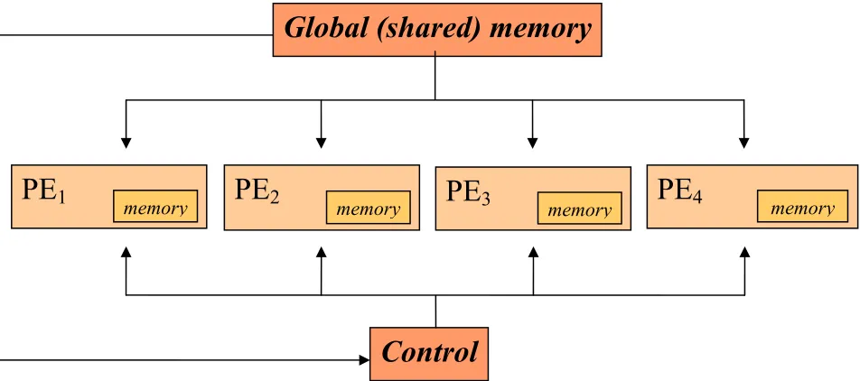
The PRAM model, as shown in Figure 2.7, allows parallel-algorithm designers to treat processsing power as an unlimited resource, much as programmers of computers with virtual memory are allowed to treat memory as an unlimited resource. It is

unrealistically simple which means it ignores the complexity of interprocessor

communication. By doing that, it can focus on the parallelism inherent in a particular computation. A PRAM consists of a control unit, global memory, and an unbounded set of processors, each with it’s own private memory. A PRAM computation begins with the input stored in global memory and a single active processing element. During each step of the computation an active, enabled processor may read a calue from a single private or global memory location, perform a single RAM operation and write into one local or may activate another processor.

Figure 2.7: The PRAM model of parallel computation

PE

PE

PE3

memory

PE

Global (shared) memory

2.5 PROCESSOR ORGANIZATIONS / TOPOLOGY

The topology of a network describes how processors are distributed and organized in it. In terms of graph, the processors are represented as nodes and the edges linking any pair of nodes in the graph are the communication links between the two processors (El-Rewini et al., 1992). Some common types of processor organizations include the mesh, binary trees, hypertree, butterfly, pyramid, hypercubes, shuffle-exchange and the De Bruijn model.

These processor organizations are evaluated according to criteria that help determine their practicality and versatility. The criteria include:

1. Diameter

The diameter of a network is the largest distance between two nodes.

2. Bisection width

The bisection width of a network is the minimum number of edges that must be removed in order to divide the network into two halves.

3. Number of edges per nodes

The number of edges per nodes should be maintained as a constant

independent of the network size. This is because it would be easier for the processor organizations to scale the system with large number of nodes.

4. Maximum edge length

In this chapter, we focus on the reconfigurable mesh (RMesh) network as a

platform for solving the task scheduling, image processing and routing problems. Mesh-based architectures have attracted strong interest because of the following reasons:

• The wiring cost is cheap as the complexity is lower compared to other models, such as the hypercube.

• It has a close match for direct mapping on many application problems, such as in task scheduling and image processing.

A regular mesh of size N×Nhas a communication diameter equals to )

1 (

2 N− . The time needed by this network to solve problem like comparing or combining data is O(N). To improve the time complexity, that is to get the most minimun computation time, researchers have studied a new architecture based on a 2 or 3 dimensional mesh which provide additional communication links between the

processors of the mesh.

2.6 RECONFIGURABLE MESH NETWORK (RMESH)

2.6.1 Reconfigurable Mesh Architecture

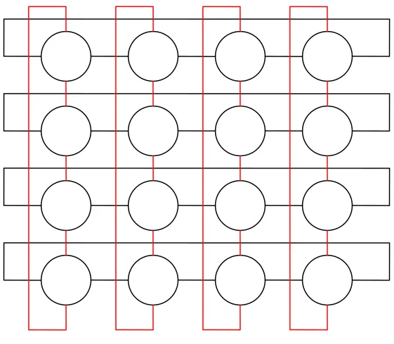
In a reconfigurable mesh network, the processors are arranged into n-dimensional arrays of processors (Olariu et al., 1993). Figure 2.8 shows a 2-dimensional RMesh. Torus, as shown in Figure 2.9 occurs when wraparound connection are present. Wraparound connection means the connection of the processors at the edge with processors at the another edge of the same row or column. For example, processors on the first row are connected through their north ports to the south ports of processors in the last row.

1 2 3 4

5 6 7 8

9 10 11 12

13 14 15 16

Figure 2.9: Torus

The computational model in Figure 2.8 shows a 4×4 network of 16 processing

elements, PE[k], for k = 1, 2, …., 16. For the n-dimensional mesh, each processing element in the network has 2n external ports. As this model is a two-dimensional network, each processing element has 4 external ports, namely, ‘North’, ‘South’, ‘East’ and ‘West’.

North Port

West Port East Port

South Port

Figure 2.10 shows a processor in the Reconfigurable Mesh network.

Communication between the processing elements in the reconfigurable mesh can be configured dynamically in one or more buses. A bus is a doubly-linked list of processing elements, with every processing element on the bus being aware of its immediate neighbors. A bus begins in a processing element, pass through a series of other processing elements and ends in another processing element. A bus that passes through all the processing elements in the network is called the global bus, otherwise it is called a local bus.

Figure 2.8 shows two local buses B(1)={2,1,5,9,13,14} and } 4 , 8 , 7 , 3 , 2 , 6 , 10 , 14 , 15 , 16 , 12 { ) 2 ( =

B , where the numbers in the lists represent the processing element numbers arranged in order from the first (starting) processing element to the last (end). As an example from the figure, communication between

] 9 [

PE and PE[13] on the bus B(1) is made possible through the link } ]. 13 [ , ]. 9 [

{PE s PE n .

2.6.2 Data Transmission in Mesh Networks

We illustrate the idea of data transmission through the diagrams in Figures 2.11a and 2.11b. In this mesh network, data transmission from PE[1] to PE[16] requires 6 hops. The path can be written as follows:

PE [1] Æ PE [5] Æ PE [9] Æ PE [13] Æ PE [14] Æ PE [15] Æ PE [16]

It can be seen that the path needs 2

(

)

1 2 3 4

5 6 7 8

9 10 11 12

13 14 15 16

1 2 3 4

5 6 7 8

9 10 11 12

13 14 15 16

Figure 2.11a: 2D mesh with fixed connection

Figure 2.11b : 2D reconfigurable mesh

However, with the reconfigurable mesh, data transmission between the two processors reduces to a constant time. Only two steps are needed by a RMesh network for the same communication between PE [1] to PE [16]. First, it needs to set the switches and recognize which port can be connected with the next processor. Second step is transfering the data by a local bus. In this case, the local bus can be writtan as

( ) {

}

Reconfigurable mesh network is created in order to provide the flexibility to change the interconnection pattern. So, it is more dynamic and easy to use. While for mesh network, it is a static network. What makes RMesh network dynamic is because of the switches it got in every Processing Elements or nodes. This switches are also known as external ports. For 2-dimensional network, there are four ports that is North, South, East and West.

e

w

n

s

w

w

w w

w w

w

n n

n n n

n n

e e

e

e e e e

s s s s

s s s

Figure 2.13: A few patterns of the switch connection.

2.7 Sorting Algorithm Example on RMesh

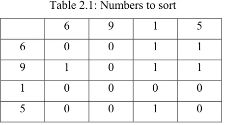
In this section, we illustrate the operation of a reconfigurable mesh network through an example in solving the sorting problem. Given a set of numbers, 6, 9, 1, 5, we need to sort these numbers in ascending order using the Rmesh model. The solution is outlined as follows:

Step 1

Table 2.1: Numbers to sort 6 9 1 5

6 0 0 1 1 9 1 0 1 1 1 0 0 0 0 5 0 0 1 0

Step 2

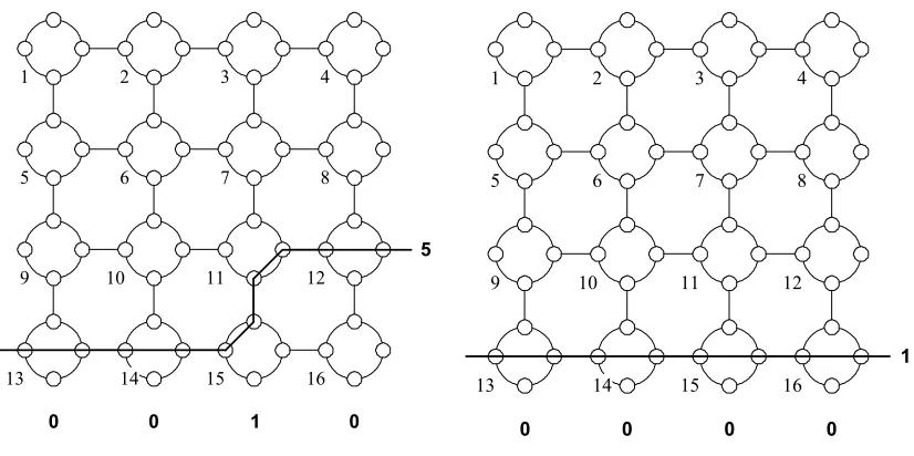
Now that we have the binary number, we can draw the Reconfigurable Mesh network. For 0, we draw a horizontal line through the nodes. While for 1, we draw a vertical line. Figure 2.14 illustrates the steps in solving this problem on Rmesh.

1 2 3 4

5 6 7 8

9 10 11 12

13 14 15 16

6

1 1

0 0

1 2 3 4

5 6 7 8

9 10 11 12

13 14 15 16

1 1

0 1

9

1 2 3 4

5 6 7 8

9 10 11 12

13 14 15 16

1 0

0 0

5

1 2 3 4

5 6 7 8

9 10 11 12

13 14 15 16

0 0

0 0

1

Number 5 at the third rank Number 1 at the last rank

Figure 2.14: Numbers in descending order from above

2.8 Summary

CHAPTER 3

DYNAMIC MULTIPROCESSOR SCHEDULING ON RMESH

3.1 Introduction

In terms of implementation, task scheduling can be classified as either static or dynamic. In static scheduling, all information regarding the states of the tasks and the processing elements are known beforehand prior to scheduling. In contrast, all this information is not available in dynamic scheduling and it is obtained on the fly, that is, as scheduling is in progress. Hence, dynamic scheduling involves extra overhead to the processing elements where a portion of the work is to determine the current states of both the tasks and the processing elements.

In this chapter, we consider the task scheduling problem on the reconfigurable mesh architecture. A reconfigurable mesh is a bus-based network of identical PE[k], for

, positioned on a rectangular array, each of which has the capability to change its

configuration dynamically according to the current processing requirements. Figure 3.1 shows a reconfigurable mesh of 20 processing elements. Due to its dynamic structure, the reconfigurable mesh computing model has attracted researchers on problems that require fast executions. These include numerically-intensive applications in computational geometry (Olariu et. al, 1994), computer vision and image processing (Olariu et. al, 1995) and algorithm designs (Nakano and Olariu, 1998).

N N

k =1,2,...,

5 4x

This chapter is organized into five sections. Section 3.1 is the introduction. Section 3.2 is an overview of the dynamic scheduling problem, while Section 3.3 describes our model which is based on the reconfigurable mesh computing model. The simulation results of our model are described in Section 3.4. Finally, Section 3.5 is the summary and conclusion.

3.2 Dynamic Task Scheduling Problem

Dynamic scheduling is often associated with real-time scheduling that involves periodic tasks and tasks with critical deadlines. This is a type of task scheduling caused by the nondeterminism in the states of the tasks and the PEs prior to their execution. Nondeterminism in a program originates from factors such as uncertainties in the number of cycles (such as loops), the and/or branches, and the variable task and arc sizes. The scheduler has very little a priori knowledge about these task characteristics and the system state estimation is obtained on the fly as the execution is in progress. This is an important step before a decision is made on how the tasks are to be distributed.

The main objective in dynamic scheduling is usually to meet the timing constraints, and performing load balancing, or a fair distribution of tasks on the PEs. Load balancing improves the system performance by reducing the mean response time of the tasks. In Lin and Raghavendran (1991), load balancing objective is classified into three main components. First, is the information rule which describes the collection and storing processes of the information used in making the decisions. Second, is the transfer rule which determines when to initiate an attempt to transfer a task and whether or not to transfer the task. Third, is the location rule which chooses the PEs to and from which tasks will be transferred. It has been shown by several researchers that with the right policy to govern these rules, a good load balancing may be achieved.

tasks arrive would take the initiative to transfer the tasks. In the server-initiative algorithms, the receiving hosts would find and locate the tasks for them. For implementing these ideas, a good load-balancing algorithm must have three components, namely, the information, transfer and placement policies. The information policy specifies the amount of load and task information made available to the decision makers. The transfer policy determines the eligibility of a task for load balancing based on the loads of the host. The placement policy decides which eligible tasks should be transferred to some selected hosts.

Tasks that arrive for scheduling are not immediately served by the PEs. Instead they will have to wait in one or more queues, depending on the scheduling technique adopted. In the first-in-first-out (FIFO) technique, one PE runs a scheduler that dispatches tasks based on the principle that tasks are executed according to their arriving time, in the order that earlier arriving tasks are executed first. Each dispatch PE maintains its own waiting queue of tasks and makes request for these tasks to be executed to the scheduler. The requests are placed on the schedule queue maintained by the scheduler. This technique aims at balancing the load among the PEs and it does not consider the communication costs between the tasks. In Chow and Kohler (1979), a queueing model has been proposed where an arriving task is routed by a task dispatcher to one of the PEs. An approximate numerical method is introduced for analyzing two-PE heterogeneous models based on an adaptive policy. This method reduces the task turnaround time by balancing the total load among the PEs. A central task dispatcher based on the single-queue multiserver queueing system is used to make decisions on load balancing. The approach is efficient enough to reduce the overhead in trying to redistribute the load based on the global state information.

Our performance index for load balancing is the mean response time of the processing elements. The response time is defined as the time taken by a processing element to response to the tasks it executes. In general, load balancing is said to be achieved when the mean response time of the tasks is minimized. A good load balancing algorithm tends to reduce the mean and standard deviation of the task response times of every processing elements in the network.

Scheduler

task arrivals

task departures

µ1

µc

µ3

µ2

λ1

λ4

λ3

λ2

PE[1]

PE[c] PE[3] PE[2]

Fig.3.2: The m/m/c queueing model

In our work, task scheduling is modeled as the Markovian queueing system. An algorithm is proposed to distribute the tasks based on the probability of a processing element receiving a task as the function of the mean response time at each interval of time and the overall mean turnaround time. Tasks arrive at different times and they form a FIFO queue. The arrival rate is assumed to follow the Poisson distribution with a mean arrival rate of

c m m/ /

In general, the mean response time R for tasks arriving at a processing element is given from the Little’s law defined in (Kobayashi, 1978), as follows:

λ

N

R= (3.1)

where is the mean number of tasks at that processing element. In a system of processing elements, the mean response time is given as follows (Kobayashi, 1978):

N n

k k k

R

λ

µ −

= 1 (3.2)

where λ_kis the mean arrival rate and µ_k is the mean service rate at the processing element k. It follows that the mean response time for the whole system is given as follows (Kobayashi, 1978):

∑

= n

k k

R n R

1 * 1

(3.3)

where

∑

≠ =

= n

k k

n

0 , 1

* ₁

λ

3.3 Reconfigurable Mesh Computing Model

3.3.1 Computational Model

The computational model is a network of 16 processing elements, , for k , as shown in Figure 3.3. Each processing element in the network has four ports, denoted as

and , which represent the north, south, east and west

communicating links respectively. These ports can be dynamically connected in pairs to suit some computational needs.

4

4x PE[k] =1,2,...,16

n k

PE[ ]. , PE[k].s, PE[k].e PE[k].w

Communication between the processing elements in the reconfigurable mesh can be configured dynamically in one or more buses. A bus is a doubly-linked list of processing elements, with every processing element on the bus being aware of its immediate neighbours. A bus begins in a processing element, pass through a series of other processing elements and ends in another processing element. A bus that passes through all the processing elements in the network is called the global bus, otherwise it is called a local bus. Figure 3.3 shows two local buses and B(1)={2,1,5,9,13,14} B(2)={12,16,15,14,10,6,2,3,7,8,4}

) 1

, where the numbers in the

lists represent the processing element numbers arranged in order from the first (starting) processing element to the last (end). As an example, from Figure 3.3, communication between

and on the bus is made possible through the link { . ]

9 [

1 2 3 4

5 6 7 8

9 10 11 12

13 14 15 16

Fig.3.3: A 4x 4 reconfigurable mesh network with two subbuses

The processing elements in a bus cooperate to solve a given problem by sending and receiving messages and data according to their controlling algorithm. A positive direction in a bus is defined as the direction from the first processing element to the last processing element, while the negative direction is the opposite. Note that the contents in the list of each bus at any given time t can change dynamically according to the current computational requirements.

3.3.2 Scheduling Model and Algorithm

In the model, assumes the duty as the controller to supervise all activities performed by other processing elements in the network. This includes gathering information about the incoming tasks, updating the information about the currently executing tasks, managing the buses and locating the positions of the PEs for task assignments.

In our model, we assume the tasks to be nonpreemptive, independent and have no precedence relationship with other tasks. Hence, the computational model does not consider the communication cost incurred as a result of data transfers between tasks. We also assume the tasks to have no hard or soft executing deadlines. At time t =0, the controller records

randomly arriving tasks, for

0 Q Q Q ≤ ≤ ₀ 0 i]. [ 0 Q

, and immediately places them in a FIFO queue, where

is a predefined maximum number of tasks allowed. Each task Task is assigned a number i and a random length, denoted as Task . The controller selects connected PEs to form the bus and assigns the tasks to the q PEs in . At this initial stage, the controller creates the bus list to consist of a single bus , that is,

Q [i]

0 q 0 ( {B length 0 ) 0 (

B B(0)

S B(0) S= )}. The PEs then start

executing their assigned tasks, and their status are updated to “busy”. Each PE broadcasts the information regarding its current execution status and the task it is executing to the controller, and the latter immediately updates this information.

This initial operation is repeated in the same way until the stopping time t is reached. At time t, random new tasks arrive and they are immediately placed in the FIFO queue. The queue line is created in such a way that every task will not miss its turn to be assigned to a PE. There are some Q tasks who failed to be assigned from the previous time slots, and these tasks are automatically in the front line. Hence, at any given time t, there are tasks in the queue, of which all Q tasks are in front of the Q tasks. In an attempt to accommodate these tasks, the controller forms buses in the list

StopTime = ( ),..., 1 (

),B B m

t

Q

w

w

t Q

Q + _{w t}

S

m ={B(0 )}.

Each bus has q connected PEs and this number may change according to the current processing requirements. The controller may add or delete the contents of each bus ,

depending on the overall state of the network. A PE in a bus that has completed executing

a task may be retained or removed from this bus, depending on the connectivity requirements for accommodating the tasks. The controller also checks the status of other PEs not in the list S. These PEs are not “busy” and may be added to the connecting buses in . At the same time, some PEs may be transferred from one bus in to another bus. In addition, the controller may also add or delete one or more buses in the list to accommodate the same processing needs.

Finally, when the buses have been configured a total of q “free” PEs are then assigned to the q tasks in the front queue. When all the tasks have been completely executed, the controller

compiles the information in its database to evaluate the mean arrival time

t t

k

λ , the mean

executing time µ_k, and the mean response time R_k of each PE[k] in the network.

S ) 0 ( )} 0 = 0 ( B t + ) (j B S

S= S

t

q j B(

R

Our algorithm for scheduling the tasks dynamically on the reconfigurable mesh is summarised as follows:

At t=0, the controller records Q0 newly arriving tasks;

The controller selects q0 connected PEs at random to form the bus B(0); The Q0 new tasks are assigned to the PEs in B(0);

The controller flags the assigned PEs in B as “busy”; The controller creates the bus list {B( ;

The controller updates the state information of the PEs in S ={ )}; for t=1 to StopTime

new tasks arrive while Q tasks still waiting;

t

Q _w

The controller places all the Q Qw tasks in the FIFO queue;

The controller checks the state information of the PEs in of the list {B(0),B(1),...,B(m)}where )⊆ :

The controller checks the state information of the PEs not in ; S The controller decides if the contents of B(j) need to change; The controller decides if the list needs to change; S

The controller selects “free” PEs, assign them to the buses in ; S The controller assigns qt PEs to the front tasks;

The controller updates the state information of the PEs in ; The controller evaluates λk, µk, and k of PE[k] in ; S

3.4 Simulation and Analysis of Results

The simulation is performed on an Intel Pentium II personal computer. A C++ Windows-based simulation program called Dynamic Scheduler on Reconfigurable Mesh (DSRM) has been developed to simulate our model. DSRM assumes the tasks to have no partial orders, no communication dependence, no timing constraints and are nonpreemptive. Figure 3.4 shows a sample run of some randomly arriving tasks on a 4 network. In DSRM, every time tick is a discrete event where between 0 to 10 randomly determined number of tasks are assumed to enter the queue waiting to be assigned to the PEs. For each task, its arrival time (randomly determined), length (randomly determined) and completion time, is displayed as a green or orange bar in the Gantt chart.

4

x t

DSRM has some flexible features which allow a user-defined mesh network sizes of m , where . In addition, DSRM also displays the status of each processor in the

network at time as a square. A green square indicates the processor is busy as it has just been assigned a task, while a red square indicates the processor is also currently busy as it is still executing a previously assigned task. A black square indicates the processor is currently idle and, therefore, is ready for assignment. Figure 3.4 shows an instance of this discrete event at . is busy as it has just been assigned with Task 98, while is also busy as it is

still executing Task 92. In contrast, is currently idle and is waiting for an assignment.

n

x

64 ,..., 2 , 1 ,n=

m

t

] 3 [ PE

20

=

t PE[7]

Fig.3.4: Sample run from DSRM

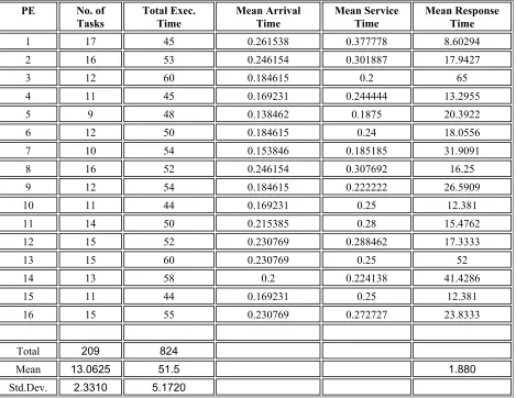
Results from a sample run of 209 successfully assigned tasks on a network are shown in Table 3.1. Due to its dynamic nature, not all the tasks that arrive at time managed to be assigned successfully on the limited number of processors. In this sample, 35 tasks failed to be assigned and this gives the overall success rate of 85.7%, which is reasonably good. In general, the overall success rate can be improved by controlling factors such as reducing the maximum number of arriving tasks at every time tick t and increasing the network size. In addition, it is possible to have a 100% success rate by bringing forward the unsuccessfully assigned tasks at time to enter the queue at time

4 4x

t

t t +1, t+2 and so on. These factors normally impose some timing constraints on the tasks, such as the execution deadline, and are presently not supported in DSRM.

lowest assignment (9). The standard deviation is 2.3310, while the overall mean response time is 1.880. The tasks have a total execution time of 824 time units, with a mean of 51.5 and a standard deviation of 5.1720 on each processor. The table also shows the performances of each processor in the network, in terms of its mean arrival time, mean service time and mean response time, which describes a reasonably good distribution.

Table 3.1: Sample run of 209 successful randomly generated tasks on 16 PEs

PE No. of Tasks

Total Exec. Time

Mean Arrival Time

Mean Service Time

Mean Response Time

1 17 45 0.261538 0.377778 8.60294

2 16 53 0.246154 0.301887 17.9427

3 12 60 0.184615 0.2 65

4 11 45 0.169231 0.244444 13.2955

5 9 48 0.138462 0.1875 20.3922

6 12 50 0.184615 0.24 18.0556

7 10 54 0.153846 0.185185 31.9091

8 16 52 0.246154 0.307692 16.25

9 12 54 0.184615 0.222222 26.5909

10 11 44 0.169231 0.25 12.381

11 14 50 0.215385 0.28 15.4762

12 15 52 0.230769 0.288462 17.3333

13 15 60 0.230769 0.25 52

14 13 58 0.2 0.224138 41.4286

15 11 44 0.169231 0.25 12.381

16 15 55 0.230769 0.272727 23.8333

Total 209 824

Mean 13.0625 51.5 1.880

3.5 Summary and Conclusion

This chapter describes dynamic task scheduling model implemented on the reconfigurable mesh computing model. The model is illustrated through our simulation program called Dynamic Simulator on Reconfigurable Mesh (DSRM) which maps a randomly generated number of tasks onto a network of processors at every unit time based on our scheduling algorithm. DSRM produces reasonably good load balancing results with a high rate of successful assigned tasks, as demonstrated in the sample run.

n

mx t

CHAPTER 4

RMESH MODEL FOR THE EDGE DETECTION PROBLEM

4.1 Introduction

This chapter presents our work in detecting the edges of an image using the reconfigurable mesh network. Edge detection is an important component of image processing which involves massive computations. Fast computers and good algorithms are some of the requirements in image processing. Due to its dynamic structure, the reconfigurable mesh computing model has attracted researchers on problems that require fast executions. These include numerically-intensive

applications in computational geometry (Olariu et. al, 1994), computer vision and image

processing (Olariu et. al, 1995) and algorithm designs (Nakano and Olariu, 1998).

4.2 Edge Detection Problem

The edges of an image form a separation line between pixels of the low intensity and the high intensity. Edge detection is a technique of getting this boundary line which holds the key to other image processing requirements, such as object recognition, image segmentation, image enhancement and image manipulation. Through edge detection, pixels can grouped according their variation in grey level or colour values based on some predefined threshold value. This information is vital to segmenting the image into two or more regions so that objects in the image can be detected or manipulated in ways appropriate to the problem.

Edge detection techniques aim to locate the edge pixels that form the objects in an image, minus the noise. Three main steps in edge detection are noise reduction, edge enhancement and edge localization. Noise reduction involves the removal of some unwanted noise pixels that sometime overshadow the real image. In edge enhancement, a filter is applied that responds strongly at edges of the image and weakly elsewhere, so that the edges may be identified as local maxima in the filter’s output. Edge localization is the final step that separates the local maxima caused by the edges or by the noise.

The Laplacian edge detection method is a second order convolution that measures the local slopes of x and of an image y f(x,y)(Effold, 2000). For an image of size q x r

, 1 , 0

, the intensity

of a pixel at coordinate (i,j) is represented in discrete form as f_ij, where i= 2,...,r−1 and

. The Laplacian of this image is defined as follows: 1 2 , 1 , 0 − = q j ,..., 2 2 2 2 2 y f x f f ∂ ∂ + ∂ ∂ =

∇ (4.1)

It follows that

1 , , 1 , , 1 , , 1

2 _{f =} fi j −2fi j + fi j ₊ fi j −2fi j + fi j

Assuming ∆x=∆y=1 (4.2) 1 , 1 , , 1 , , 1 2 ₄ − + − + − + + + =

∇ f f_{i j} f_{i j} f_{i j} f_{i j} f_{i j}

and this produces the x high pass filter [4]:

(4.3)           − − − − 0 1 0 1 4 1 0 1 0

Similarly, the high pass filter is given by the matrix [4]: y

(4.4)           − − − − − − − − 1 1 1 1 8 1 1 1 1

The sequential Laplacian method for detecting the edges of an image is given as follows:

/* Sequential Laplacian algorithm */

z

Let = number of edges;

Let (xE,yE) be the x and output, respectively; y Set the edge threshold ET be a constant;

Set (xH,yH) as the left-hand corner pixel of the output image; for j=0 to q

for i=0 to r

Set fij= pixel value at (i,j); Set z=0;

for j=1 to q−1 for i=1 to r−1

) 4

( _{, +1}− _−1, + _, − _+1, − _{, −1}

=abs f_{i j} f_{i j} f_{i j} f_{i j} f_{i j}

xE ;

) 8

(− _{−1, +1} − _{, +1}− _{+1, +1}− _−1, + _, − _+1, − _{−1, −1}− _{, −1} − _{+1, −1}

=abs f_{i j} f_{i j} f_{i j} f_{i j} f_{i j} f_{i j} f_{i j} f_{i j} f_{i j}

yE ;

Set xyE=xE+yE;

if xyE≥ET

z++;

4.3 Reconfigurable Mesh Computing Model

Our computing platform consists of a network of 16 processing elements arranged in reconfigurable meshes. A suitable realization for this model is the message-passing transputer-based system where each transputer represents a processing element with a processing element and a memory module each, and has communication links with other transputers.

Figure 4.2 shows a 4 x 4 network of 16 processing elements, , for the rows

and columns . Each processing element in the network is capable of

executing some arithmetic and logic operations. In addition, each processing element has some memory and four ports for communication with other PEs, denoted as

and , which represent the north, south, east and west links respectively.

These ports can be dynamically connected in pairs to suit some computational needs. ] , [i j PE

j i PE , ]. 3 , 2 , 1 , 0 = i e j i PE[ , ].

3 , 2 , 1 , 0 = j n

[ , PE[i, j].s,

w j i PE[, ].

0,0 0,1 0,2 0,3

1,0 1,1 1,2 1,3

2,0 2,1 2,2 2,3

3,0 3,1 3,2 3,3

Communication between processing elements in the reconfigurable mesh can be configured dynamically in one or more buses. A bus is a doubly-linked list of processing elements, with every processing element on the bus being aware of its immediate neighbors. A bus begins in a processing element, pass through a series of processing elements and ends in another processing element. A bus that passes through all the processing elements in the network is called the global bus, otherwise it is called a local bus. Figure 4.2 shows two local buses

and , where the numbers in the lists

represent the processing element numbers arranged in order from the first (starting) processing

element to the last (end). As an example from the figure, communication between and

on the bus is denotated as { .

} 14 , 13 , 9 , 5 , 1 , 2 { ) 1 ( = B ] 0 , 3 [ PE B } 4 , 8 , 7 , 3 , 2 , 6 , 10 , 14 , 15 , 16 , 12 { ) 2 ( = B ]. 0 , 3 [ , ]. 0 , 2

[ s PE n

PE ] 0 , 2 [ PE ) 1 ( }

The processing elements in a bus cooperate to solve a given problem by sending and receiving messages and data according to their controlling algorithm. A positive direction in a bus is defined as the direction from the first processing element to the last processing element, while the negative direction is the opposite. Note that the contents in the list of each bus at any given time t can change dynamically according to the current computational requirements.

4.4 RM Model for Detecting the Edges

Our computing model is based on a n reconfigurable mesh network. As the model resembles

a rectangular array, the computing platform is suitable for mapping the pixels of a

n x

r

q x image

directly for fast executions. For this purpose, we assume n<q and n<r.

The Laplacian convolution of a qx image involves scanning the r portion of the

image beginning from the top left-hand corner of the image to the right, and continues downward continuously until the bottom right-hand corner is reached. This windowing process computes the second derivatives of with respect to

n n x

f x and , given as and in Equation (4.1),

respectively. The convolution output at (i,j) is then given as

y xE xyE yE yE + xE

= . This value is

) ]. [ , ]. [

(E z x E z y

ij

f

, where is the edge number, otherwise the pixel is not an edge. Some initial

assignments: is the intensity of the pixel at (i,j),

z

ET is the edge threshold and (

indicates the home coordinate where the binary edge image needs to be constructed.

) ,yH xH

) ,

(xE yE x

) ,

(xH yH

T T 4 q n ) 1 1 + − ) 1 , 1 − + 8 _,

− fi j fi j

yE i f yE xyE xH 600 x

It follows that our parallel algorithm using the RM model is summarized as follows:

/* Parallel Laplacian algorithm using a nx n reconfigurable mesh */ Let be the and output, respectively; y

Set as the left-hand corner pixel of the output image; Let the intensity at pixel (i,j) be f_ij;

At PE[0,0], set the number of edges z=0;

At PE[0,0], set the edge threshold ET to be a constant; PE[0,0] broadcasts E southbound to PE[0,k], for k=1,2,…, n; PE[0,k] broadcasts E westbound to PE[h,k], for h=1,2,…, n; for u=0 to step , where

for v=0 to r₄ step , where n r₄ =n

 

par j=u to u+n par i=v to v+ n

Set h = 1 + i% n; Set k = 1 + j% n;

PE[h,k] evaluates xE=abs(fi_,j fi−_1,j +4fi_,j − fi+_1,j − fi_,j− and

(− _{1, +1} − _{, +1}− _{+1, +1}− _−1, + − _+1, − _{−1, −1}− _{, −1} −

=abs _j f_{i j} f_{i j} f_{i j} f_{i j} f_{i j} f_{i j} ;

PE[h,k] evaluates xyE=xE+ ; if ≥ET at PE[h,k]

PE[h,k] broadcasts a positive flag to PE[0,0]; At PE[0,0], set z←z+1 with the positive flag; At PE[h,k], set E[z].x= +i and E[z].y =xH +j;

At PE[h,k], plot the edge pixel at (E[z].x,E[z].y);

As can be seen, the above algorithm has the complexity of , against the sequential

complexity of O . Finally, a C++ program to simulate the above algorithm has been

developed. The program detects edges of up to 800 bitmap images, to produce their

corresponding binary images.

) / (_{qr n}2

O

4.5 Summary and Conclusion

We have presented a parallel Laplacian method using the reconfigurable mesh network for detecting the edges of an image . The algorithm is implemented in a C++ program that simulates

networks of various sizes to support up to 800 bitmap images. The method has the

complexity of .

n

n x x 600

) / (_{qr n}2

CHAPTER 5

SINGLE-ROW ROUTING USING THE ENHANCED SIMULATED

ANNEALING TECHNIQUE

5.1 Introduction

A typical VLSI design involves extensive conductor routings which make all the necessary wirings and interconnections between the PCB modules, such as pins, vias, and backplanes. In very large systems, the number of interconnections between the microscopic components in the circuitry may exceed thousands or millions. Therefore, the need to optimize wire routing and interconnection in the circuit is crucial for efficient design. Hence, various routing techniques such as single-row routing, maze routing, line probe routing, channel routing, cellular routing and river routing have been applied to help in the designs.