by Using Bayesian Approach with Application
Thanoon Y. Thanoon
Northern Technical University, Technical College of Management, Mosul, Iraq [email protected]
Robiah Adnan
Department of Mathematical Science, Faculty of Science Universiti Teknologi Malaysia,01318Skudai, Johor, Malaysia [email protected]
Abstract
In this paper, Bayesian analysis is used in nonlinear structural equation models with two population of data and the Gibbs sampling method is applied for estimation and model comparison. Hidden continuous normal distribution (censored normal distribution) is used to solve the problem of ordered categorical data in Bayesian multiple group SEMs and compared with the method that treats ordered categorical variables as a continuous normal distribution. Statistical inferences, which involve the estimation of parameters and their standard errors, and residuals analyses for testing the posited model are discussed. The proposed procedure is illustrated using real data with the results obtained from the WinBUGS program.
Keywords: Structural Equation Models, Bayesian Analysis, Censored Normal Distribution, Gibbs Sampling, Ordered Categorical Variables.
1. Introduction
Structural equation models (SEMs) (Bollen and Paxton, 1998; Lee, 2007) constitute a statistical methodology for modelling multivariate correlated data to assess the interrelationships among observed and latent variables.
At present, most statistical theory and computer software in the field of SEMs are based on models that involve nonlinear relationships among the manifest and the latent variables. More statistically sound methods for nonlinear SEMs and factor analysis have been proposed by Lee & Tang, (2006), Lee & Tang, (2007), Cai et al., (2008(, Lee et al.,(2010), Thanoon & Adnan, (2015), Thanoon & Adnan, (2016a), Thanoon & Adnan, (2016b), Thanoon & Adnan, (2016c), Thanoon & Adnan, (2016d), Thanoon et al., (2017).
the basis of simulated observations from the Gibbs sampler. Efficiency and flexibility of the proposed Bayesian procedure are illustrated by some simulation results and a real-life example. Song and Lee, (2006) discussed multiple group nonlinear structural equation models with missing continuous and dichotomous data that involve data that are missing at random using maximum likelihood approach, as well as, he demonstrated the newly developed methods for estimation and model comparison by a simulation study and a real data application. Lee, (2007) used underlying latent continuous normal distribution with truncation to solve the problem of ordered categorical variables in Bayesian multiple group nonlinear structural equation models, as well as, Gibbs sampling method is used to estimate the parameters. Lu et al., (2012) used Bayesian analysis of multiple group nonlinear structural equation models with application to behavioral finance and treated the ordered categorical variables as a continuous normal distribution. The proposed method is used to investigate the relationships among all identified influential factors that have an impact on the motivation for insider trading within the framework of behavioural finance (Thanoon and Adnan, 2015).
For the structural equation model with ordered categorical data, an important generalization is to extend the model to permit analysis of multiple groups or populations of individuals simultaneously. Multiple group analysis is important in various applications, such as cross-cultural research. It is very interesting to investigate whether the measurement items (which are often on Likert scales of a categorical nature) are of different cultures. To achieve this goal requires statistical methods for testing various hypotheses in the multi-sample structural equation models with ordered categorical variables.
The Bayesian approach is developed with the Gibbs sampler (Geman & Geman, 1984) algorithm, in which the continuous latent measurements and the latent variables in different groups are treated as hypothetical missing data.Non-informative priors are used for the thresholds and conjugate priors are used for the structural parameters.
Theoretically, the importance of generalizing nonlinear structural equation models to nonlinear models that include nonlinear terms of the latent variables is obvious. Practically, nonlinear relationships, such as quadratic and interaction terms, among the variables are important in establishing the substantive theory in many areas. The rapid growth of SEMs is due to the demand of subtle models and the related statistical methods for solving complex research problems in various fields.
A major breakthrough for posterior simulation is the idea of data augmentation proposed by Tanner and Wong (1987). The strategy is to treat latent quantities as hypothetical missing data and to augment the observed data with them so that the posterior distribution based on the complete data set is relatively easy to analyze. The feature that makes SEMs different from the common regression model and the simultaneous equation model is the existence of random latent variables.
The data augmentation provides a useful approach to cope with the problem that is induced by latent variables. By augmenting the observed variables in complicated SEMs with the latent variables that are treated as hypothetical missing data, we can obtain the
generalizing nonlinear structural equation models to nonlinear models that include nonlinear terms of the latent variables is obvious. Practically, nonlinear relationships, such as quadratic and interaction terms, among the variables are important in establishing the substantive theory in many areas. The rapid growth of SEMs is due to the demand of subtle models and the related statistical methods for solving complex research problems in various fields.
The main objective of this paper is to propose a Bayesian approach for analysing multiple group nonlinear SEMs with ordered categorical variables. The Deviance Information Criterion (DIC; see Spiegelhalter et al., 2002) will be used for model comparison.
The main idea in handling the ordered categorical variables in the Bayesian analysis is to treat the underlying latent continuous measurements as hypothetical missing data and augment them with the observed data in the posterior analysis.
The paper is organized as follows. The Model Description is described in Section 2. The Bayesian estimation of multiple group structural equation models that contain nonlinear models is described in Section 3. The normal distribution is presented in section 4. The truncated normal distribution is explained in Section 5. The censored normal distribution is presented in Section 6. The comparison of models using DIC is described in Section 7. A real example study is presented in Section 8. Analysis of a real data are discussed in Section 9. The results and discussion are described in Section 10, and some concluding remarks are given in Section 11.
2. Model Description
Consider a set of G populations which may be different nations, states or regions, cultural or socio-economic groups, groups receiving different treatments, etc. The definition of the multiple group structural equation models is given by:
For g 1, 2,...,G , and i 1, 2,..., Ng, let yi( )g be the p1 random vector of observed
variables that relate to the ith observation in the gth group. For eachg 1, 2,...,G , ( )g
i
y
is related to latent variables in a q1 random vector wi( )g by the next measurement equation: (Lee & Song, 2012; Lee, 2007; Lee et al., 2010)
( ) ( ) ( ) ( ) ( )
, 1,...,
g g g g g
i i i i n
y (1)
Where ( )g
u is the intercepts vector, ( )g is the parameter matrix of regression coefficients
that reflect the relation of manifest variables in ( )g i
y with the latent variables in ( )g i
w , and ( )g
i
is a random vector of the measurement errors. It is presumed that ( )g i
w and ( )g
i
are independent while the distribution of i( )g is
( )
[0, g ]
variables in ( )g i
to ( )g i
we consider a nonlinear SEM with the following nonlinear structural equation:
( ) ( ) ( ) ( ) ( ) ( ) ( ) * ( ) ( )
( ) ( )
g g g g g g g g g
i i H i i w H wi i
(2)
Where ( )g and ( )g are unknown parameter matrices, and ( )g i
is the random vector of error measurements that is independent of ( )g
i
; ( ) ( ) ( )
( , )
g g g
w
,
* ( ) ( )T ( )
(wig ) ( ig , ( ig ) )T T
H H and ( ) ( ) ( )
1
( ig ) ( ( ig ),..., a( ig ))T
H h h , in which the hs are nonzero and known differentiable functions that include polynomials.
It is expected that the vector-valued functions H and H* do not depend on g. However, different groups can require different linear or nonlinear function of i( )g by major appropriate of H or H* and assigning zero values to appropriate elements in( )g . For instance, let wi( )g (i( )g ,i( )1g ,i( )2g )T forg 1, 2. Suppose that the structural equations in the first and second groups are given as:
(1) (1) (1) (1) (1) (1) (1) (1) (1)
1 1 2 2 3 1 2
i i i i i i
(3)
(2) (2) (2) (2) (2) (2) (2) (2) (2)
1 1 2 2 4 1 1
i i i i i i
(4)
To define these structural equations, we consider
( ) ( ) ( ) ( ) ( ) ( ) ( )
1 2 1 2 1 1
( ig ) ( ig , ig , ig ig , ig ig )T
H , (1) ( 1(1), 2(1), 3(1), 0)and
(2) (2) (2) (2)
1 2 4
( , ,0, )
.
In reality, the models in different groups typically have similar linear and nonlinear of
( )g i
. For handling really complicated different nonlinear functions in the models, this assumption can be relaxed with minor changes. Likewise, as for the models, it is assumed that ( )g is a non-singular matrix where the determinant is not dependent on elements in( )g
. It is further assumed that ( )g i
is distributed as (g)
[ , ]
N 0 and ( )g i
is distributedN[ ,0( )g ], where ( )g is a diagonal covariance matrix.
To handle the ordered categorical outcomes, suppose that ( )g i
y is an s1 subvector of unobservable continuous responses, the information of which is reflected by an observable ordered categorical vector ( )g
i
z . In a generic sense, an ordered categorical variable ( )g
m
z is defined with its underlying latent continuous random variable ( )g m
y by:
( ) ( )
1,1 1,1 1
( ) ( )
, , 1
( ) ( ) ( )
( ) 1
1 ( ) ( ) ( ) ( ) ( ) g g z z g g
s zs s zs
g g g
g
g
g g g g
s s if
y z zwhere { ( ),1 ( ),2 ... ( ),b ( ),b 1 }
m m
g g g g
m m m m
is the set of threshold parameters that define the categories, and bmis the number of categories for the ordered categorical variable zm( )g . Note that for each ordered categorical variable, the number of thresholds is the same for each group. However, the categories can be unequally spaced under this formulation.
It has been pointed out by (Lee et al., 1990) that single-sample models with ordered categorical variables are not identified without imposing identification conditions. This is also the case for multi-sample models. To solve this problem, we use the common method (see, for example, Lee et al., 1995; Shi & Lee, 1998( of fixing some thresholds at pre-assigned values. For convenience, it is assumed that the positions of the fixed elements are the same for each group.
Multiple Group data come from a comparatively smaller number of groups of populations. The number of observations within each group is normally large and assumed independent. The primary purpose of the multiple group data analysis is to investigate the similarities or differences among the models in the different groups. As a consequence, the statistical inferences emphasized in analyzing multiple group of the SEMs are different from those in analyzing two-level SEMs. Analysis of the multiple group is a major issue in structural equation modeling because it is useful for investigating the behaviors of different groups for example of employees, cultures, treatment groups, and so on. Though, the testing of hypotheses about the different invariances among the models with different groups is the focus point.
This issue can be described as a model comparison problem, and also effectively addressed by the Bayes factor or DIC in a Bayesian approach. The benefit of the Bayesian model comparison over the Bayes factor or DIC is that the hypotheses of nonnested models can be compared. Hence, it is not necessary to follow hypotheses hierarchy to assess the invariance for the SEMs in different groups (Song & Lee, 2012; Wang & Wang, 2012).
3. Bayesian Analysis of Multiple Group Nonlinear Structural Equation Models
Allow Z (z1,...,zn) stand for the matrix of ordered categorical data. Then, allow
1
( ,..., n)
Y y y and (w1,...,wn) be the latent continuous measurements and latent variables matrices. Such that, the observed data, as represented by [Z] is improved according to the latent data [Y,] through the posterior analysis. Thus in order to define the Bayesian approach for the proposed SEM, allow
to act as the vector containing unknown parameters. In explanation, the Bayesian approach, would define p( ) such that is considered a random with prior distribution and prior density function. Thus, the the related assumptions can be based on the observed data for Z and p( ) . So, allow Let( , )
p Z represent the joint probability density function of both Z and
with reference to different Mk. Based on a well-known identity in probability,This yields the posterior density function p( | Z) , or unknown parameters. It also employs the use of sample information and prior knowledge, via the likelihood function
(Z | )
p , and the prior density function p( ) . It should be noted, however, that p(Z | ) is dependent on sample size, where p( ) is not. As such, for problems with a large sample, p( ) is less significant and p( | Z) , the posterior density function, is more relevant, as it is most similar to the likelihood function p(Z | ) . So, both the Bayesian approach and ML model are asymptotically equivalent, and thus contain the same optimal asymptotical properties. However, continue to note that p( ) is significant with regard to the Bayesian approach when the sample size is reduced or when the information derived from Z is ordered categorical data.
In this paper, MCMC methods are applied by letting yi act as an unobserved variable, which corresponds with the manifest ordered categorical variables, as they are found in
i
z . Also, one must allow Y (y1,...,yn) and (w1,...,wn). When drawing a
sufficient, and generally large, body of observations If we can draw a sufficiently large number of observations, represented by ( ) ( ) ( )
{( t ,t ,Y t );t 1,..., }T , from the joint posterior distribution, defined by p( , ,Y | Z), then the Bayesian estimate for
as well as any standard error estimates can be derived from the sample mean and variance matrices, respectively.1 ( ) 1 ( ) ( )
1 1
, var( | ) ( 1) ( )( ) .
T T
t t t
t t
T Z T
(7)This means that it is necessary to specifically identify the prior distribution for the related components in
, even if developing the conditional distribution, ( | ,Y Z, ). In generally, during Bayesian analysis, the conjugate prior distributions have proven to be both malleable and suitable to the purpose (Broemeling, 1985). This kind of prior distribution has been widely applied to many Bayesian analysis in structural equation models, (see (Lee and Song, 2004; Song and Lee, 2007)).Hence, the following well-known conjugate prior distributions are used:
0 0 0 0 0 0
1 1
0 0 0 0
( ) [ , ], ( ) [ , ], ( | ) [ , ],
( ) [ , ], ( ) [ , ]
k k k k k k k k
q k k k
p N H p N H p N H
p W R p Gamma
(8)
Given the definition that p( ) is the probability of p( ) , and that p( ) is distributed according to, k , which is the kth diagonal element of ,k and, given that k are the kth rows of and respectively. The following can be derived:
2 2
0 ( 01,..., 0p),
H diag and 0, 0k, 0k,0k,0k, 0, 0k,H0,H0k, and R0 are
assumption have on Bayesian estimations remains small, even when a large sample size is used. The results are helpful when working to use computer modeling with the Gibbs sampler. More specifically, when using the Bayesian approach, it is necessary to evaluate the posterior distribution[ , , Z], but the distribution can become relatively complex. So, in order to correctly demonstrate the characteristics, an increased number of observations are drawn, so that the related empirical distribution of the resulting observations remains consistent with the true distribution. The Gibbs sampler makes an excellent candidate for this process, according to (Geman and Geman, 1984), because it can simulate , and , all from the conditional distribution. However, as a result of the existence of ordered categorical variables in this case, the related conditional distributions can be made too complex to easily derive or simulating data from them. This encourages the additional escalation of Y, the latent matrix, in the posterior analysis, and motivates attention to the joint posterior distribution[ , , , Y Z]. To garner observations of this posterior distribution, using the Gibbs sampler, it is essential to begin with the starting values (0) (0) (0) (0)
( , , ,Y ). The following procedure is then implemented to simulate (1) (1) (1) (1)
( , , ,Y ) and so on. More specifically at the mth reiteration of the current values ( ) ( ) ( ) ( )
, , ,
m m m m
Y
.
1. Generate (m1) from ( 1) ( ) ( )
( m , m , m , Z)
p Y
2. Generate (m1) from p( (m1),(m),Y (m), Z)
3. Generate ( 1) ( 1)
(m ,Y m )from ( 1) ( 1)
( , Y | m , m , )
p Z (9)
The cycle, as previously defined, will give us ( 1) ( 1) ( 1) ( 1)
( m , m , m , m )
Y
, only occurring after the mth repetition. So, as m approaches infinity, the joint distribution of the value of ( ) ( ) ( ) ( )
( m , m , m,Y m )can be proven to move toward the joint posterior distribution [ , , , Y Z] (see Geman and Geman, (1984); Geyer, (1992((.
The sequences in which the quantities are replicated from the joint posterior distribution are then used during the calculation of the Bayesian estimates and other
similarly related statistics. 4. The Normal Distribution
To indicate that * 2
( , ).
y N y*has the pdf:
2 *
* 2 1 1
( | , ) exp
2 2
y
f y
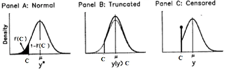
which is plotted in Panel A Figure 1, the cdf is
*
* * *
( | , ) ( | , ) Pr( )
y
F y f z dz Y y
so that
* * *
Pr(Y y ) 1 F y( | , )
( | , )
F c is the shaded region in Panel A Figure 1 and 1F c( | , ) is the region to the right of c.
When µ=0 and ζ=1, the standard normal distribution is written in the simplified notation:
* *
* *
( ) ( | 0, 1) ( ) ( | 0, 1)
y f y
y F y
Any normal distribution, regardless of its mean µ and variance ζ2
, can be written as a function of the standard normal distribution. The pdf can be written as
2
* *
* 1 1 1
( | , ) exp 2 2
y y
f y
(11)
and the cdf of y* can be written as
*
* *
Pr(Y y ) y
(12)
so that,
*
* *
Pr(Y y ) 1 y
Hidden continuous normal distribution. 5. The Truncated Normal Distribution
region, while ignoring all cases in the shaded region. The truncated pdf is created by dividing the pdf of the original distribution by the region to the right of c. This forces the resulting distribution to have an area of 1: (Scott Long, 1997)
* * ( | , ) ( | , , ) Pr( ) f y
f y y c
Y c
(13)
The truncated distribution is shown in Panel B Figure 1 by the solid line. The mass of the shaded region has been distributed over the region to the right of c, making the curve slightly higher over this region. This is seen by comparing the solid curve for the truncated distribution to the dotted line for the normal distribution without truncation. Using the results from Equations 12 and 13, we can write the truncated distribution as
* *
1 1
( | , , ) 1
y y
f y y c
c c
Given that the left-hand side of the distribution has been truncated, E y y( | c) must be larger than E(y*) = µ. Specifically, if y* is normal
( | )
c
c
E y y c
c (14)
where (.) (.) (.)
A sampling distribution is truncated if for some reason, we never observe cases above or below a specified point, although in the permissible range of observations the data follow a standard distribution. It is very important to realise that the I(,) construct is not appropriate for truncated distributions with unknown parameters, since the generated likelihood term will ignore the truncation and be incorrect. However, the I(,) construct can be used when specifying truncated prior distributions with no unknown parameters. The indicator I(,) is used for censoring not for truncation because we have unobserved dependent variables in the SEMs and we can't use truncation with this type of variables (Lunnet al., 2012).
6. The Censored Normal Distribution
A data point is a censored observation when we do not know its exact value, but we do know that it lies above or below a point c, say, or within a specified interval.
the probability that a given observation from the untruncated population falls within the parameters for a population of interest (Greene, 2003).
When a distribution is censored on the left, observations with values at or below c are set to cy:
* *
*
y
y if y c
y
c if y c
Most often, cy= c, but other values such as zero are also useful. Panel C of Figure 1 plots
a censored normal variables, where the censored observation is indicated by the spike at y= c. From Equation 12, we know that if y* is normal, then the probability of an observation being censored is
Pr(Censored)= Pr(y* c) c
and the probability of a case not being censored is Pr(Uncensored) = *
Pr(y c)= 1 c c
Thus, the expected value of a censored variable equals
E(y) = [Pr(Uncensored) × E (y|y>c)]+ [Pr(Censored) × E (y|y=cy)]
y
c c c
c
(15)
where the last equality uses Equation 14 consider how the expected value of the censored value depends on c. As c approaches ∞, the probability of being censored approaches 1 and E(y) approaches the censoring value cy. As c approaches -∞, the probability of being
censored approaches 0 and E(y) approaches the uncensored mean µ (Scott Long, 1997).
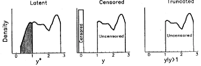
Figure 2. Latent, Censored, and Truncation Variables
7. Model Comparison
A model comparison statistic DIC (see Spiegelhalter et al., 2002) is a generalization of the Akaike Information Criterion (AIC; Akaike, (1973). Under a competing model Mk with a vector of unknown parameters k , the DIC is computed as follows:
( ) ,
k k k
DIC D d
(16)
where D(k) measures the goodness of fit of the model, and is defined as
( ) { 2log ( | , ) | }.
k
k k k
D p Z M Z (17)
Here, dkis the effective number of parameters in Mk, and is defined as
[ 2log ( | , ) | ] 2log ( | ).
k
k k k
d p Z M Z f Z (18)
in which is the Bayesian estimate of . Let {k( )t :t 1,..., }T be a sample of observations simulated from the posterior distribution. The expectations in Equations (17)
and (18) can be estimated as follows:
( )
1
2
{ 2 log ( | , ) | } log ( | , ).
k
T
t
k k k k
t
p Z M Z p Z M
T
(19) In Bayesian SEMs, the model with the smaller DIC value is selected.
8. Real Example
participants were followed up every six months after the baseline interview for three consecutive years ) Wang & Wang, 2012).
Again, the BSI-18 scale was used for model demonstration. The three dimensions of psychiatric disorders measured by the BSI-18 are: somatization (SOM), depression (DEP), and anxiety (ANX). Each of the three subscales was measured by six items, respectively. All the BSI-18 items are measured on a fivepoint Likert scale (1, not at all; 2, a little bit; 3, moderately; 4, quite a bit; 5, extremely). All subscales of the BSI-18 have excellent reliabilities with Cronbach’s alpha greater than 0.80 in the populations under study.
9. Analysis of Real Data
A real data study is presented here to give some idea of the empirical performance of the proposed Bayesian approach in which 18 manifest variables are related to two basic latent variables ( , i1, i2) from multiple group nonlinear SEMs defined in Equation 21 and Equation 22 respectively. Hence, some quadratic and interaction effects of the latent variables are considered. To illustrate the Bayesian methods in analysing linear and nonlinear structural equation models with ordered categorical variables, we use a simulated data set that is related to random vectors with G=1,2,
( ) ( ) ( ) ( )
1 2 18
( , ,..., )
g g g g
i i i i
z z z z , let (g) (g) (g) (g)
1 2 18
( , ,..., )
i i i i
y y y y be the latent continuous random vector which corresponds to the ordinal variables zi(g)1 ,zi(g)2,...,zi( )18g where zi(g),i 1,..., n are ordered categorical variables that are related to (3) latent variables wi(g)( i(g), i(g)1 , i(g)2),
(g) (g) (g) (g)
1 2 18
( , ,..., )
i i i i
, with the following values of the parameters in
(g) (g) (g) (g)
1 2 18
( , ,..., )
and (g) (1(g),2(g),...,15(g) )
(1) (1) (1) (1) (1) * * * * * *
* * * * * * *
21 31 41 51 61
(g) (1) * * * * * * (1) (1) (1) (1) (1) * * * * * *
82 92 102 112 122
* * * * * * * * * * * * (1) (1) (1) (1) (1)
143 153 163 173 183
( 2)
0 0 0 0 0 0
1 0 0 0 0 0 0
0 0 0 0 0 0 1 0 0 0 0 0 0 ,
0 0 0 0 0 0 0 0 0 0 0 0 1
( 2) ( 2) ( 2) ( 2) ( 2) * * * * * *
* * * * * * *
21 31 41 51 61
( 2) ( 2) ( 2) ( 2) ( 2)
* * * * * * * * * * * *
82 92 102 112 122
* * * * * * * * * * * * ( 2) ( 2) ( 2) ( 2) ( 2)
143 153 163 173 183
0 0 0 0 0 0
1 0 0 0 0 0 0
0 0 0 0 0 0 1 0 0 0 0 0 0 .
0 0 0 0 0 0 0 0 0 0 0 0 1
(1) ( 2)
(g) (1) 11 ( 2) 11
(1) (1) ( 2) ( 2)
21 22 21 22
,
.
(20)Where parameters with an asterisk are treated as fixed for identifying the model.
The relationships of the latent variables in wi ( i, 1 ,i 2i)are assessed by the nonlinear structural equation which described in equation.
(1) (1) (1) (1) (1) (1) (1) (1) (1) (1) (1) (1) (1) (1) (1)
1 1 2 2 3 1 2 4 1 1 5 2 2 ,
i i i i i i i i i i
(21)
(2) (2) (2) (2) (2) (2) (2) (2) (2) (2) (2) (2) (2) ( 2) (2)
1 1 2 2 3 1 2 4 1 1 5 2 2 .
i i i i i i i i i i
The following accurate prior inputs of the hyperparameter values in the conjugate prior distributions of the parameters are considered:
Prior I. Elements in0,0k and 0k in Equations (8) are set equal to 1;
1
0 8
R H0u,H0k and H0kare taken to be 0.25 times the identity matrices; 0k 10
, 0k 8 ,0 30.
Prior II. Elements in0,0k and 0k in Equations (8) are set equal to 0.5;
1
0 8
R H0u,H0k and H0k are taken to be 0.25 times the identity matrices; 0k 10
, 0k 8,0 30.
The prior is informative and can have a significant effect on the parameter estimates for a small sample size case.
A data set (n1=200, n2=200) was analyzed by WinBUGS. In comparing the Bayesian
analyses of structural equation models with data, the MCMC procedure for analysing data required more iterations to converge. Bayesian estimates were obtained from T=10000. Iterations after discarding 4000 burn-in iterations with ordered categorical variables. The WinBUGS software (Spiegelhalter et al., 2003) can produce Bayesianestimates of the parameters in some two-level nonlinear SEMs. To demonstrate this, we apply WinBUGS to analyse the current aids data based on (Model 5) with different prior inputs.
10. Results and Discussion
The objective of this section is to present results of a simulation study to reveal the empirical performances of the Bayesian estimates and the DIC for model comparison. For linear and nonlinear SEMs we have the following proposed models:
1 1 2 2 3 3 4 1 2
1 1 2 2 3 3 4 1 3
1 1 2 2 3 3 4 2 3
2
1 1 2 2 3 3 4 1 2 5 2
1 1 2 2 3 3 4 1
1: ,
2 : ,
3 : ,
4 : ,
5 :
i i i i i i i
i i i i i i i
i i i i i i i
i i i i i i i i
i i i i i
Model Model Model Model Model
i2 5 4 i1 i1 4 i2 i3i,
(23)
account the ordered categorical nature is necessary
.
Hence, clearly, routinely treating ordered categorical variables as normal may lead to erroneous conclusions (see Lee et al., 1990; Olsson, 1979).A better approach for assessing this kind of discrete data is to treat them as observations obtained from a hidden continuous normal distribution (censored normal distribution) with a threshold specification. Second, the current analysis was conducted under the normality assumption of the observed variables in the model. However, this assumption is likely to be violated. Developing a linear & nonlinear Bayesian approach with hidden continuous normal distribution (right censored normal distribution, left censored normal distribution) to relax the normality assumption in SEMs may represent a future research topic.
mu.y2[3] chains 1:2
iteration
1 2500 5000 7500 10000
-2.0 -1.5 -1.0 -0.5 0.0
lam1[5] chains 1:2
iteration
1 2500 5000 7500 10000
-1.0 0.0 1.0 2.0 3.0
g am2[1] chains 1:2
iteration
1 2500 5000 7500 10000
-2.0 0.0 2.0 4.0
phx1[2,2] chains 1:2
iteration
1 2500 5000 7500 10000
0.0 1.0 2.0 3.0
mu.y2[3] chains 1:2
iteration
1 2500 5000 7500 10000
1.6 1.8 2.0 2.2 2.4
lam1[5] chains 1:2
iteration
1 2500 5000 7500 10000
-1.0 0.0 1.0 2.0 3.0 4.0
gam2[1] chains 1:2
iteration
1 2500 5000 7500 10000
-1.0 0.0 1.0 2.0 3.0
phx1[2,2] chains 1:2
iteration
1 2500 5000 7500 10000
0.0 0.5 1.0 1.5
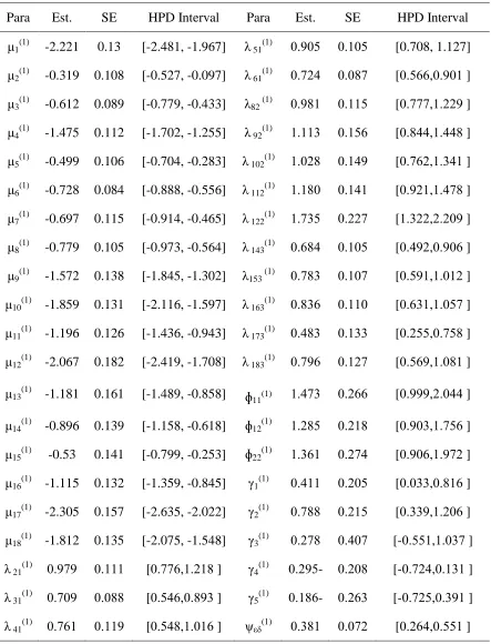
Table 1: Bayesian Estimation of Multiple Group Nonlinear SEM with Ordered Categorical Variables of First Group under Prior I
Para Est. SE HPD Interval Para Est. SE HPD Interval μ1(1) -2.221 0.13 [-2.481, -1.967] λ 51(1) 8.980 8.180 [0.708, 1.127]
μ2(1) -0.319 0.108 [-0.527, -0.097] λ 61(1) 8.7.0 8.807 [8.000,8.981 ]
μ3(1) -0.612 0.089 [-0.779, -0.433] λ82 (1) 8.901 8.110 [8.777,1...9 ]
μ4(1) -1.475 0.112 [-1.702, -1.255] λ 92(1) 1.113 8.100 [8.000,1.000 ]
μ5(1) -0.499 0.106 [-0.704, -0.283] λ 102(1) 1.8.0 8.109 [8.70.,1.301 ]
μ6(1) -0.728 0.084 [-0.888, -0.556] λ 112(1) 1.108 8.101 [8.9.1,1.070 ]
μ7(1) -0.697 0.115 [-0.914, -0.465] λ 122(1) 1.730 8...7 [1.3..,...89 ]
μ8(1) -0.779 0.105 [-0.973, -0.564] λ 143(1) 8.000 8.180 [8.09.,8.980 ]
μ9(1) -1.572 0.138 [-1.845, -1.302] λ153 (1) 8.703 8.187 [8.091,1.81. ]
μ10(1) -1.859 0.131 [-2.116, -1.597] λ 163(1) 8.030 8.118 [8.031,1.807 ]
μ11(1) -1.196 0.126 [-1.436, -0.943] λ 173(1) 8.003 8.133 [8..00,8.700 ]
μ12(1) -2.067 0.182 [-2.419, -1.708] λ 183(1) 8.790 8.1.7 [8.009,1.801 ]
μ13(1) -1.181 0.161 [-1.489, -0.858] ɸ11(1) 1.073 8..00 [8.999,..800 ]
μ14(1) -0.896 0.139 [-1.158, -0.618] ɸ12(1) 1..00 8..10 [8.983,1.700 ]
μ15(1) -0.53 0.141 [-0.799, -0.253] ɸ22(1) 1.301 8..70 [8.980,1.97. ]
μ16(1) -1.115 0.132 [-1.359, -0.845] γ1(1) 8.011 8..80 [8.833,8.010 ]
μ17(1) -2.305 0.157 [-2.635, -2.022] γ2(1) 8.700 8..10 [8.339,1..80 ]
μ18(1) -1.812 0.135 [-2.075, -1.548] γ3(1) 8..70 8.087 [-8.001,1.837 ]
λ 21(1) 8.979 8.111 [8.770,1..10 ] γ4(1) 8..90- 8..80 [-8.7.0,8.131 ]
λ 31(1) 8.789 8.800 [8.000,8.093 ] γ5(1) 8.100- 8..03 [-8.7.0,8.391 ]
λ 41(1) 8.701 8.119 [8.000,1.810 ] ψεδ(1) 8.301 8.87. [8..00,8.001 ]
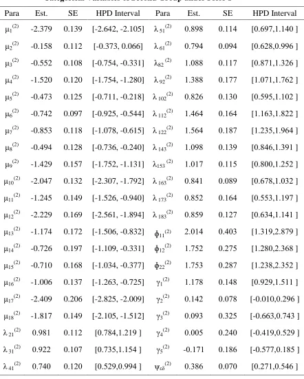
Table 2: Bayesian Estimation of Multiple Group Nonlinear SEM with Ordered Categorical Variables of Second Group under Prior I
Para Est. SE HPD Interval Para Est. SE HPD Interval μ1(2) -2.379 0.139 [-2.642, -2.105] λ 51(2) 8.090 8.110 [8.097,1.108 ]
μ2(2) -0.158 0.112 [-0.373, 0.066] λ 61(2) 8.790 8.890 [8.0.0,8.990 ]
μ3(2) -0.552 0.108 [-0.754, -0.331] λ82 (2) 1.800 8.117 [8.071,1.3.0 ]
μ4(2) -1.520 0.120 [-1.754, -1.280] λ 92(2) 1.300 8.177 [1.871,1.70. ]
μ5(2) -0.473 0.125 [-0.711, -0.218] λ 102(2) 8.0.0 8.138 [8.090,1.18. ]
μ6(2) -0.742 0.097 [-0.925, -0.544] λ 112(2) 1.000 8.100 [1.103,1.0.. ]
μ7(2) -0.853 0.118 [-1.078, -0.615] λ 122(2) 1.000 8.107 [1..30,1.900 ]
μ8(2) -0.494 0.128 [-0.736, -0.240] λ 143(2) 1.890 8.139 [8.000,1.391 ]
μ9(2) -1.429 0.157 [-1.752, -1.131] λ153 (2) 1.817 8.110 [8.088,1..0. ]
μ10(2) -2.047 0.132 [-2.307, -1.792] λ 163(2) 8.001 8.809 [8.070,1.83. ]
μ11(2) -1.245 0.149 [-1.526, -0.940] λ 173(2) 8.00. 8.100 [8.003,1.197 ]
μ12(2) -2.229 0.169 [-2.561, -1.894] λ 183(2) 8.009 8.1.7 [8.030,1.101 ]
μ13(2) -1.174 0.172 [-1.506, -0.832] ɸ11(2) ..810 8.083 [1.319,..079 ]
μ14(2) -0.726 0.197 [-1.109, -0.331] ɸ12(2) 1.70. 8..70 [1..08,..300 ]
μ15(2) -0.710 0.168 [-1.034, -0.377] ɸ22(2) 1.703 8..07 [1..30,..30. ]
μ16(2) -1.006 0.137 [-1.263, -0.725] γ1(2) 1.170 8.100 [8.9.9,1.011 ]
μ17(2) -2.409 0.206 [-2.825, -2.009] γ2(2) 8.10. 8.870 [-0.010,8..90 ]
μ18(2) -1.817 0.149 [-2.105, -1.512] γ3(2) 8.893 8.3.0 [-0.663,8.703 ]
λ 21(2) 8.901 8.11. [8.700,1..19 ] γ4(2) 8.880 8..08 [-0.419,8.0.9 ]
λ 31(2) 8.9.. 8.187 [8.730,1.100 ] γ5(2) -8.171 8.100 [-0.577,8.100 ]
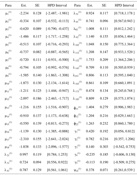
Table 3: Bayesian Estimation of Multiple Group Nonlinear SEM with Ordered Categorical Variables of First Group under Prior II
Para Est. SE HPD Interval Para Est. SE HPD Interval μ1(1) -2.234 0.128 [-2.487, -1.981] λ 51(1) 8.9.0 8.117 [8.710,1.170 ]
μ2(1) -0.334 0.107 [-0.532, -0.113] λ 61(1) 8.701 8.890 [8.007,8.903 ]
μ3(1) -0.620 0.089 [-0.790, -0.437] λ82 (1) 1.880 8.111 [8.01.,1..0. ]
μ4(1) -1.486 0.117 [-1.717, -1.258] λ 92(1) 1.108 8.100 [8.000,1.000 ]
μ5(1) -0.513 0.107 [-0.716, -0.293] λ 102(1) 1.800 8.108 [8.770,1.300 ]
μ6(1) -0.737 0.082 [-0.887, -0.565] λ 112(1) 1..80 8.107 [8.933,1.0.8 ]
μ7(1) -0.720 0.111 [-0.931, -0.500] λ 122(1) 1.703 8..89 [1.300,...80 ]
μ8(1) -0.794 0.105 [-0.992, -0.576] λ 143(1) 8.789 8.118 [8.080,8.939 ]
μ9(1) -1.585 0.140 [-1.863, -1.308] λ153 (1) 8.080 8.113 [8.090,1.808 ]
μ10(1) -1.873 0.130 [-2.134, -1.614] λ 163(1) 8.001 8.189 [8.008,1.891 ]
μ11(1) -1.211 0.125 [-1.446, -0.947] λ 173(1) 8.070 8.130 [8..00,8.700 ]
μ12(1) -2.097 0.186 [-2.463, -1.717] λ 183(1) 8.089 8.1.9 [8.070,1.870 ]
μ13(1) -1.216 0.155 [-1.516, -0.907] ɸ11(1) 1.080 8..79 [8.980,1.903 ]
μ14(1) -0.910 0.137 [-1.173, -0.638] ɸ12(1) 1..80 8..10 [8.0.9,1.003 ]
μ15(1) -0.550 0.139 [-0.813, -0.273] ɸ22(1) 1..03 8..3. [8.008,1.708 ]
μ16(1) -1.139 0.130 [-1.385, -0.888] γ1(1) 0.420 0.192 [0.056, 0.812]
μ17(1) -2.310 0.155 [-2.641, -2.024] γ2(1) 0.782 0.216 [0.357, 1.206]
μ18(1) -1.838 0.133 [-2.096, -1.577] γ3(1) 0.140 0.303 [-0.542, 0.753]
λ 21(1) 0.997 0.119 [0.784, 1.253] γ4(1) -0.235 0.185 [-0.606, 0.130]
λ 31(1) 0.724 0.094 [0.556, 0.922] γ5(1) -0.113 0.190 [-0.509, 0.275]
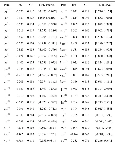
Table 4: Bayesian Estimation of Multiple Group Nonlinear SEM with Ordered Categorical Variables of Second Group under Prior II
Para Est. SE HPD Interval Para Est. SE HPD Interval μ1(1) -2.370 0.146 [-2.673, -2.097] λ 51(1) 0.921 0.111 [0.716, 1.153]
μ2(1) -0.139 0.126 [-0.384, 0.107] λ 61(1) 0.814 0.092 [0.652, 1.010]
μ3(1) -0.536 0.114 [-0.766, -0.320] λ82 (1) 1.089 0.115 [0.872, 1.323]
μ4(1) -1.511 0.119 [-1.755, -1.286] λ 92(1) 1.362 0.166 [1.062, 1.718]
μ5(1) -0.452 0.133 [-0.708, -0.187] λ 102(1) 0.826 0.131 [0.588, 1.106]
μ6(1) -0.723 0.108 [-0.939, -0.511] λ 112(1) 1.460 0.152 [1.180, 1.767]
μ7(1) -0.829 0.135 [-1.102, -0.579] λ 122(1) 1.581 0.185 [1.254, 1.975]
μ8(1) -0.474 0.140 [-0.752, -0.205] λ 143(1) 1.100 0.133 [0.860, 1.378]
μ9(1) -1.400 0.173 [-1.751, -1.073] λ153 (1) 1.035 0.116 [0.834, 1.291]
μ10(1) -2.038 0.143 [-2.335, -1.768] λ 163(1) 0.845 0.094 [0.673, 1.049]
μ11(1) -1.219 0.172 [-1.563, -0.892] λ 173(1) 0.851 0.167 [0.553, 1.211]
μ12(1) -2.203 0.186 [-2.574, -1.862] λ 183(1) 0.856 0.118 [0.648, 1.111]
μ13(1) -1.167 0.168 [-1.490, -0.832] ɸ11(1) 1.972 0.415 [1.321, 2.919]
μ14(1) -0.713 0.203 [-1.102, -0.292] ɸ12(1) 1.757 0.322 [1.217, 2.498]
μ15(1) -0.686 0.178 [-1.020, -0.322] ɸ22(1) 1.794 0.347 [1.213, 2.551]
μ16(1) -0.995 0.141 [-1.267, -0.712] γ1(1) 1.194 0.145 [0.915, 1.484]
μ17(1) -2.389 0.204 [-2.812, -2.023] γ2(1) 0.139 0.078 [-0.012, 0.299]
μ18(1) -1.799 0.154 [-2.102, -1.499] γ3(1) 0.096 0.346 [-0.566, 0.642]
λ 21(1) 1.880 8.180 [8.08.,1..10 ] γ4(1) 0.004 0.230 [-0.417, 0.465]
λ 31(1) 8.90. 8.183 [8.70.,1.107 ] γ5(1) -0.166 0.242 [-0.584, 0.297]
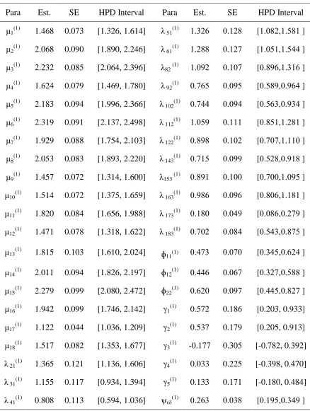
Table 5: Bayesian Estimation of Multiple Group Nonlinear SEM with Ordered Categorical Variables Treated as a Continuous Normal of First Group under Prior I
Para Est. SE HPD Interval Para Est. SE HPD Interval μ1(1) 1.468 0.073 [1.326, 1.614] λ 51(1) 1.3.0 8.1.0 [1.80.,1.001 ]
μ2(1) 2.068 0.090 [1.890, 2.246] λ 61(1) 1..00 8.1.7 [1.801,1.000 ]
μ3(1) 2.232 0.085 [2.064, 2.396] λ82 (1) 1.89. 8.187 [8.090,1.310 ]
μ4(1) 1.624 0.079 [1.469, 1.780] λ 92(1) 8.700 8.890 [8.009,8.900 ]
μ5(1) 2.183 0.094 [1.996, 2.366] λ 102(1) 8.700 8.890 [8.003,8.930 ]
μ6(1) 2.319 0.091 [2.137, 2.498] λ 112(1) 1.809 8.111 [8.001,1..01 ]
μ7(1) 1.929 0.088 [1.754, 2.103] λ 122(1) 8.090 8.18. [8.787,1.118 ]
μ8(1) 2.053 0.083 [1.893, 2.220] λ 143(1) 8.710 8.899 [8.0.0,8.910 ]
μ9(1) 1.457 0.072 [1.314, 1.600] λ153 (1) 8.091 8.188 [8.788,1.890 ]
μ10(1) 1.514 0.072 [1.375, 1.659] λ 163(1) 8.900 8.890 [8.080,1.101 ]
μ11(1) 1.820 0.084 [1.656, 1.988] λ 173(1) 8.108 8.809 [8.800,8..79 ]
μ12(1) 1.471 0.078 [1.318, 1.622] λ 183(1) 8.78. 8.800 [8.003,8.070 ]
μ13(1) 1.815 0.103 [1.610, 2.024] ɸ11(1) 8.073 8.878 [8.300,8.0.0 ]
μ14(1) 2.011 0.094 [1.826, 2.197] ɸ12(1) 8.000 8.807 [8.3.7,8.000 ]
μ15(1) 2.279 0.099 [2.080, 2.472] ɸ22(1) 8.0.8 8.897 [8.000,8.0.7 ]
μ16(1) 1.942 0.099 [1.746, 2.142] γ1(1) 0.572 0.186 [0.203, 0.933]
μ17(1) 1.122 0.044 [1.036, 1.209] γ2(1) 0.537 0.179 [0.205, 0.913]
μ18(1) 1.517 0.082 [1.353, 1.677] γ3(1) -0.177 0.305 [-0.782, 0.392]
λ 21(1) 1.365 0.121 [1.136, 1.606] γ4(1) 0.033 0.225 [-0.398, 0.470]
λ 31(1) 1.155 0.117 [0.934, 1.394] γ5(1) 0.133 0.171 [-0.180, 0.484]
Table 6: Bayesian Estimation of Multiple Group Nonlinear SEM with Ordered Categorical Variables Treated as a Continuous Normal of Second Group under Prior I
Para Est. SE HPD Interval Para Est. SE HPD Interval μ1(2) 1.3.1 8.801 [1..83,1.00. ] λ 51(2) 1.372 0.139 [1.104, 1.653]
μ2(2) ..8.0 8.808 [1.078,..101 ] λ 61(2) 1.480 0.131 [1.234, 1.748]
μ3(2) 1.999 8.80. [1.030,..107 ] λ82 (2) 1.168 0.118 [0.945, 1.415]
μ4(2) 1.000 8.800 [1.300,1.017 ] λ 92(2) 0.937 0.094 [0.761, 1.127]
μ5(2) ..803 8.807 [1.911,...03 ] λ 102(2) 0.594 0.081 [0.441, 0.757]
μ6(2) ..80. 8.803 [1.98.,... ] λ 112(2) 1.182 0.107 [0.981, 1.400]
μ7(2) 1.719 8.877 [1.07.,1.071 ] λ 122(2) 0.798 0.083 [0.643, 0.974]
μ8(2) ..1.0 8.800 [1.900,...91 ] λ 143(2) 0.876 0.089 [0.710, 1.054]
μ9(2) 1.011 8.878 [1..71,1.000 ] λ153 (2) 0.931 0.084 [0.772, 1.099]
μ10(2) 1.370 8.808 [1..00,1.090 ] λ 163(2) 0.972 0.078 [0.827, 1.131]
μ11(2) 1.0.0 8.870 [1.073,1.770 ] λ 173(2) 0.276 0.052 [0.176, 0.380]
μ12(2) 1.380 8.808 [1.109,1.0.0 ] λ 183(2) 0.683 0.069 [0.551, 0.823]
μ13(2) 1.000 8.800 [1.307,1.7.1 ] ɸ11(2) 0.412 0.061 [0.307, 0.546]
μ14(2) 1.7.1 8.89. [1.00.,1.98. ] ɸ12(2) 0.416 0.060 [0.311, 0.544]
μ15(2) 1.707 8.800 [1.010,1.900 ] ɸ22(2) 0.617 0.096 [0.446, 0.827]
μ16(2) 1.70. 8.803 [1.009,1.913 ] γ1(2) 1.021 0.129 [0.782, 1.296]
μ17(2) 1.809 8.808 [8.971,1.107 ] γ2(2) 0.013 0.062 [-0.110, 0.135]
μ18(2) 1.33. 8.871 [1.190,1.073 ] γ3(2) -0.192 0.331 [-0.767, 0.444]
λ 21(2) 1.017 8.1.0 [1..79,1.701 ] γ4(2) 0.242 0.262 [-0.283, 0.742]
λ 31(2) 1.0.0 8.1.9 [1..70,1.700 ] γ5(2) 0.257 0.184 [-0.100, 0.578]
Table 7: Bayesian Estimation of Multiple Group Nonlinear SEM with Ordered Categorical Variables Treated as a Continuous Normal of First Group under Prior II
Para Est. SE HPD Interval Para Est. SE HPD Interval μ1(1) 1.470 0.072 [1.329, 1.611] λ 51(1) 1.332 0.129 [1.090, 1.595]
μ2(1) 2.070 0.088 [1.897, 2.247] λ 61(1) 1.293 0.127 [1.058, 1.557]
μ3(1) 2.234 0.085 [2.066, 2.400] λ82 (1) 1.097 0.107 [0.898, 1.311]
μ4(1) 1.626 0.079 [1.470, 1.780] λ 92(1) 0.768 0.094 [0.591, 0.959]
μ5(1) 2.185 0.094 [1.997, 2.370] λ 102(1) 0.745 0.096 [0.568, 0.944]
μ6(1) 2.321 0.090 [2.138, 2.497] λ 112(1) 1.066 0.113 [0.857, 1.297]
μ7(1) 1.931 0.088 [1.760, 2.106] λ 122(1) 0.900 0.101 [0.712, 1.107]
μ8(1) 2.055 0.082 [1.897, 2.219] λ 143(1) 0.716 0.099 [0.529, 0.919]
μ9(1) 1.459 0.071 [1.319, 1.602] λ153 (1) 0.892 0.100 [0.703, 1.093]
μ10(1) 1.516 0.071 [1.379, 1.655] λ 163(1) 0.987 0.096 [0.809, 1.180]
μ11(1) 1.822 0.083 [1.662, 1.984] λ 173(1) 0.180 0.050 [0.086, 0.279]
μ12(1) 1.473 0.077 [1.321, 1.625] λ 183(1) 0.703 0.085 [0.543, 0.875]
μ13(1) 1.815 0.102 [1.617, 2.021] ɸ11(1) 0.468 0.069 [0.347, 0.611]
μ14(1) 2.011 0.093 [1.826, 2.195] ɸ12(1) 0.442 0.066 [0.324, 0.583]
μ15(1) 2.280 0.098 [2.090, 2.472] ɸ22(1) 0.615 0.099 [0.443, 0.825]
μ16(1) 1.943 0.098 [1.755, 2.141] γ1(1) 0.573 0.187 [0.207, 0.951]
μ17(1) 1.122 0.044 [1.035, 1.209] γ2(1) 0.539 0.182 [0.209, 0.933]
μ18(1) 1.517 0.081 [1.358, 1.678] γ3(1) -0.179 0.308 [-0.795, 0.391]
λ 21(1) 1.374 0.122 [1.146, 1.622] γ4(1) 0.038 0.229 [-0.406, 0.491]
λ 31(1) 1.159 0.117 [0.935, 1.399] γ5(1) 0.133 0.174 [-0.180, 0.484]
Table 8: Bayesian Estimation of Multiple Group Nonlinear SEM with Ordered Categorical Treated as a Continuous Normal Variables of Second Group under Prior II
Para Est. SE HPD Interval Para Est. SE HPD Interval μ1(1) 1.319 0.061 [1.200, 1.436] λ 51(1) 1.368 0.137 [1.105, 1.645]
μ2(1) 2.023 0.079 [1.871, 2.179] λ 61(1) 1.475 0.129 [1.235, 1.749]
μ3(1) 1.996 0.079 [1.842, 2.152] λ82 (1) 1.165 0.120 [0.939, 1.411]
μ4(1) 1.484 0.067 [1.353, 1.614] λ 92(1) 0.935 0.096 [0.753, 1.130]
μ5(1) 2.080 0.086 [1.913, 2.248] λ 102(1) 0.594 0.081 [0.439, 0.759]
μ6(1) 2.060 0.081 [1.901, 2.217] λ 112(1) 1.177 0.109 [0.976, 1.408]
μ7(1) 1.716 0.078 [1.561, 1.869] λ 122(1) 0.797 0.083 [0.644, 0.972]
μ8(1) 2.122 0.085 [1.951, 2.288] λ 143(1) 0.876 0.089 [0.706, 1.053]
μ9(1) 1.409 0.070 [1.271, 1.547] λ153 (1) 0.931 0.084 [0.770, 1.100]
μ10(1) 1.376 0.060 [1.257, 1.494] λ 163(1) 0.973 0.078 [0.828, 1.134]
μ11(1) 1.622 0.078 [1.475, 1.775] λ 173(1) 0.276 0.052 [0.175, 0.380]
μ12(1) 1.306 0.060 [1.190, 1.423] λ 183(1) 0.683 0.070 [0.552, 0.824]
μ13(1) 1.553 0.086 [1.385, 1.723] ɸ11(1) 0.414 0.061 [0.306, 0.544]
μ14(1) 1.720 0.092 [1.542, 1.900] ɸ12(1) 0.419 0.063 [0.311, 0.556]
μ15(1) 1.786 0.086 [1.620, 1.957] ɸ22(1) 0.621 0.099 [0.446, 0.838]
μ16(1) 1.751 0.083 [1.590, 1.916] γ1(1) 1.016 0.130 [0.776, 1.290]
μ17(1) 1.068 0.051 [0.969, 1.167] γ2(1) 0.012 0.063 [-0.114, 0.136]
μ18(1) 1.332 0.071 [1.192, 1.471] γ3(1) -0.203 0.330 [-0.760, 0.463]
λ 21(1) 1.513 0.125 [1.279, 1.770] γ4(1) 0.234 0.260 [-0.271, 0.746]
λ 31(1) 1.519 0.128 [1.278, 1.784] γ5(1) 0.268 0.190 [-0.104, 0.596]
Table 9: Performance of Deviance Information Criterion DIC for Multiple Group SEMs under Prior I
Ordered
Categorical Normal Group 1, n=200 7815.310 9581.190 Group 2, n=200 6755.430 8969.070
Total 14570.700 18550.300
Table 10: Performance of Deviance Information Criterion DIC for Multiple Group SEMs under Prior II
Ordered
Categorical Normal Group 1, n=200 7820.740 9575.550 Group 2, n=200 6756.540 8964.210
Total 14577.300 18539.800
The estimated multiple group nonlinear structural equation in prior I is given by
(1) (1) (1) (1) (1) (1) (1) (1) (1)
1 2 1 2 1 1 2 2
0.411 0.788 0.287 0.295 0.186 ,
i i i i i i i i i
(24)
(2) (2) (2) (2) (2) (2) (2) (2) (2)
1 2 1 2 1 1 2 2
1.178 0.142 0.093 0.005 0.171 .
i i i i i i i i i
(25)
The estimated multiple group nonlinear structural equation in prior II is given by
(1) (1) (1) (1) (1) (1) (1) (1) (1)
1 2 1 2 1 1 2 2
0.420 0.782 0.140 0.235 0.113 ,
i i i i i i i i i
(26)
(2) (2) (2) (2) (2) (2) (2) (2) (2)
1 2 1 2 1 1 2 2
1.194 0.139 0.096 0.004 0.166 .
i i i i i i i i i
(27)
The results corresponding to the first and second groups under Type I inputs, and ordered categorical variables are reported in Tables (1:2). We observed that the SE values in the first group are smaller than the SE values for the second group. However, it is expected that the empirical performance would be worse with the second group.
The results corresponding to the first and second groups under Type II inputs, and ordered categorical variables are reported in Tables (3:4). We observed that SE values in the first group are smaller than the SE values for the second group. However, it is expected that the empirical performance would be worse with the second group.
The results corresponding to the first and second groups under Type II inputs, and ordered categorical variables when treated as a continuous normal distribution are reported in Tables (7:8). We observed that the SE values in the second group are smaller than the SE values for the first group. However, it is expected that the empirical performance would be worse with the first group. We noted that most of the SE values in ordered categorical variables whan treated as a continuous normal variables are less than the SE values when treated as a ordered categorical variables.
The HPD intervals of all the parameters were computed. We observed that the performances of the HPD intervals are satisfactory for ordered categorical variables when treated as a continuous normal variables.
To reveal the performance of DIC for model comparison, we reanalysed the data sets via a nonlinear structural equation model with interaction term in the structural equation (model 5). The DIC values obtained were compared to those obtained under the correct model. Results are presented in Table 9 and Table 10.
The DIC values are very close in prior I and prior II when using ordered categorical variables. In addition, the DIC values are very close in prior I and prior II when using continuous normal distribution. The model fitting DIC in Group 2 is less than the DIC value in Group 1 in prior I and II and in the ordered categorical variables; when treated as a continuous normal distribution so the model fitting is better in Group 2. As a result, we observed the performance of DIC is not satisfactory and would be worse under ordered categorical variables when trated as a continuous normal distribution However, it performs very well for the ordered categorical variables. However, routinely treating ordered categorical variables as normal may lead to erroneous conclusions (see Lee et al., 1990; Olsson, 1979).
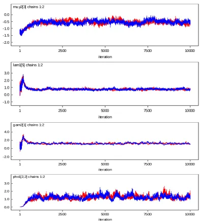
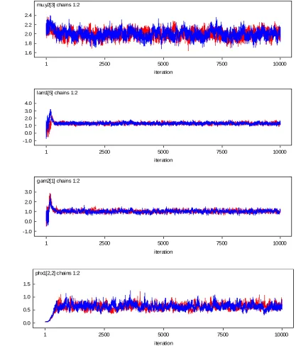
Convergence of the Gibbs sampler are monitored by the plots of several simulated sequences of the individual parameters with different starting values and are presented in Figures 4 and 5 respectively. Bayesian estimates were obtained from T=10000 iterations after discarding 4000 burn-in iterations in linear and nonlinear SEMs.
11. Conclusions and Recommendations
Models involving multiple group nonlinear effects are very common in social and behavioural sciences. The purpose of this analysis was to use multiple group NSEMs to obtain all the estimated parameters and to solve the problem of ordered categorical variables by using hidden continuous normal distribution. However, this assumption is likely to be violated in many practical applications. Developing a non-parametric Bayesian approach to relax the normality assumption in multiple group NSEMs may represent a future research topic.
technically demanding and not well understood. In this paper, a Bayesian approach is proposed for analysing multiple group nonlinear models with ordered categorical variables. In addition to point estimation, we provide statistical methods to obtain standard deviations estimates, and model comparison using the Deviance Information Criterion (DIC). Owing to the complexity of the proposed model. As we have seen, difficulties arising from the nonlinear causal relationships among the latent variables and the discrete nature of ordered categorical data manifest variables are alleviated by data augmentation with some MCMC methods. More specifically, the basic idea of our development was inspired by following the common strategy from recent work in statistical computing (see Rubin, 1991) that formulated the underlying complicated problem, so that when augmenting the real observed data with the hypothetical missing data the analysis would be relatively easy with the complete data. This strategy is very powerful and can be applied to other more complex models. The incorrectly treating indicator I as a truncated normal distribution see ( Spiegelhalter et al., 2003) and (Lunn et al., 2009).
real example studies is conducted, not only to reveal the empirical performance of the Bayesian approach, but also to show that incorrectly treating ordered categorical as a continuous normal distribution, and vice versa, would produce misleading results.
References
1. Akaike, H. (1973). Information theory and an extension of the maximum likelihood principle. Paper presented at the Second international symposium on information theory.
2. Bollen, K. A., & Paxton, P. (1998). Interactions of latent variables in structural equation models. Structural Equation Modeling, 5, 267-293.
3. Broemeling, L. D. (1985). Bayesian analysis of linear models: Dekker New York. 4. Cai, J.-H., Song, X.-Y., & Lee, S.-Y. (2008). Bayesian Analysis of Nonlinear Structural Equation Models with Mixed Continuous, Ordered and Unordered Categorical, and Nonignorable Missing Data. Statistics and its Interface, 1, 99-114.
5. Lunn, D., Spiegelhalter, D., Thomas, A. and Best, N. (2009). The BUGS project: Evolution, critique and future directions. Statistics in medicine, 28(25), 3049-3067 .
6. Geman, S., & Geman, D. (1984). Stochastic relaxation,Gibbs distribution,and the Bayesian restoration of images. IEEE Transactions on Pattern Analysis and Machine Intelligence(6), 721-741.
7. Geyer, C. J. (1992). Practical markov chain monte carlo. Statistical Science, 473-483.
8. Greene, W. H. (2003). Econometric Analysis: Pearson Education India.
10. Lee, S.-Y. and Song, X.-Y. (2012). Basic and Advanced Structural Equation Models for Medical and Behavioural Sciences. Hoboken: Wiley.
11. Lee, S.-Y. (2006). Bayesian Analysis of Nonlinear Structural Equation Models with Nonignorable Missing Data. Psychometrika, 71(3), 541-564. doi: 10.1007/s11336-006-1177-1
12. Lee, S.-Y. (2007). Structural Equation Modeling : A Bayesian Approach. Chichester, England; Hoboken, NJ: Wiley.
13. Lee, S.-Y., Poon, W.-Y., & Bentler, P. (1990). Full maximum likelihood analysis of structural equation models with polytomous variables. Statistics & probability letters, 9(1), 91-97.
14. Lee, S.-Y., & Shi, J.-Q. (2000). Bayesian Analysis of Structural Equation Model With Fixed Covariates. Structural Equation Modeling: A Multidisciplinary Journal, 7(3), 411-430. doi: 10.1207/s15328007sem0703_3
15. Lee, S.-Y., & Song, X.-Y. (2004). Evaluation of the Bayesian and maximum likelihood approaches in analyzing structural equation models with small sample sizes. Multivariate Behavioral Research, 39(4), 653-686.
16. Lee, S.-Y., Song, X.-Y., & Cai, J.-H. (2010). A Bayesian Approach for Nonlinear Structural Equation Models with Dichotomous Variables Using Logit and Probit Links. Structural Equation Modeling, 17(2), 280-302.
17. Lee, S.-Y., Song, X.-Y., & Tang, N.-S. (2007). Bayesian Methods for Analyzing Structural Equation Models With Covariates, Interaction, and Quadratic Latent Variables. Structural Equation Modeling: A Multidisciplinary Journal, 14(3), 404-434. doi: 10.1080/10705510701301511
18. Lee, S.-Y., & Tang, N.-S. (2006). Analysis of nonlinear structural equation models with nonignorable missing covariates and ordered categorical data. Statistica Sinica, 16(4), 1117.
19. Lee, S.-Y., Poon, W. Y., & Bentler, P. M. (1995). A two‐stage estimation of structural equation models with continuous and polytomous variables. British Journal of Mathematical and Statistical Psychology, 48(2), 339-358.
20. Lee, X.-Y. and Song, X.-Y. (2002). A Bayesian Approach for Multigroup Nonlinear Factor Analysis. Structural Equation Modeling, 9(4), 523–553.
21. Lee, X.-Y. and Song, X.-Y. (2004). Bayesian Analysis of Two-Level Nonlinear Structural
22. Equation Models with Continuous and Polytomous Data. British Journal of Mathematical and Statistical Psychology, 57, 29–52.
23. Lu, B., Song, X.-Y. and Li, X.-D. (2012). Bayesian Analysis of Multi-Group Nonlinear Structural Equation Models with Application to Behavioral Finance. Quantitative Finance, 12(3), 477-488. doi: 10.1080/14697680903369500
25. Lunn, D., Spiegelhalter, D., Thomas, A. and Best, N. (2009). The BUGS project: Evolution, critique and future directions. Statistics in medicine, 28(25), 3049-3067.
26. Olsson, U. (1979). Maximum likelihood estimation of the polychoric correlation coefficient. Psychometrika, 44(4), 443-460.
27. Rubin, D. B. (1991). EM and beyond. Psychometrika, 56(2), 241-254.
28. Schumacker, R. E., & Marcoulides, G. A. (1998). Interaction and nonlinear effects in structural equation modeling: Lawrence Erlbaum Associates Publishers. 29. Scott Long, J. (1997). Regression Models for Categorical and Limited Dependent
Variables. Advanced quantitative techniques in the social sciences, 7.
30. Shi, J.-Q., & Lee, S.-Y. (1998). Bayesian sampling-based approach for factor analysis model with continuous and polytomous data. British Journal of Mathematical and Statistical Psychology, 51, 233-252.
31. Song, X.-Y., Lu, Z.-H., Hser, Y.-I., & Lee, S.-Y. (2011). A Bayesian Approach for Analyzing Longitudinal Structural Equation Models. Structural Equation Modeling: A Multidisciplinary Journal, 18(2), 183-194. doi: 10.1080/10705511.2011.557331
32. Song, X.-Y., & Lee, S.-Y. (2007). Bayesian analysis of latent variable models with nonignorable missing outcomes from exponential family. Statistics in medicine, 26, 681–693.
33. Spiegelhalter, D., Thomas, A., Best, N., & Lunn, D. (2003). Winbugs user manual. Medical Research Council Biostatistics Unit, Cambridge.
34. Spiegelhalter, D. J., Best, N. G., Carlin, B. P.,, & & van der Linde, A. (2002). Bayesian Measures of Model Complexity and Fit (with Discussion). Journal of the Royal Statistical Society, Series B, 64(4), 583-639.
35. Tanner, M. A. and Wong, W. H. (1987). The calculation of posterior distributions by data augmentation. Journal of the American statistical Association, 82(398), 528-540.
36. Thanoon, T. Y.& Adnan, R.(2015). Bayesian Analysis of Multiple Group Nonlinear Structural Equation Models with Ordered Categorical and Dichotomous Variables: A Survey. Research Journal of Mathematical and Statistical Sciences. Vol. 3(12), 5-15.
37. Thanoon, T. Y.& Adnan, R.(2016a). Bayesian Analysis of Linear and Nonlinear Latent Variable Models with Fixed Covariate and Ordered Categorical Data. Pakistan Journal of Statistics and Operation Research, 12(1), 125-140. 38. Thanoon, T. Y., & Adnan, R. (2016b). Model Comparison of Linear and
39. [38] Thanoon, T. Y., & Adnan, R. (2016c). Bayesian Multi-Sample Nonlinear Structural Equation Models with Mixed Ordered Categorical and Dichotomous Variables. Journal of Applied Probability and Statistics, 11(2), 1-16.
40. [39] Thanoon, Thanoon Y., and Robiah Adnan. (2016d). Comparison between Bayesian structural equation models with ordered categorical data. AIP Conference Proceedings. Vol. 1750. No. 1. AIP Publishing.
41. [40] Thanoon, T. Y., Adnan, R., & Md Jedi, M. A. B. (2017). Model comparison of Bayesian structural equation models with mixed ordered categorical and dichotomous data. Journal of Statistics and Management Systems, 20(1), 113-131. doi:10.1080/09720510.2016.1238111.
42. [41] Wang, J., & Wang, X. (2012). Structural Equation Modeling: Applications Using Mplus: John Wiley & Sons.
43. [42] Wooldridge, J. M. (2010). Econometric Analysis of Cross Section and Panel Data: MIT press.