Analytic Approximate Solution for the KdV Equation
with the Homotopy Analysis Method
1
Mojtaba Nazari,2
Faisal Salah and3
Zainal Abdul Aziz 1,3Department of Mathematical Sciences
Faculty of Science, Universiti Teknologi Malaysia 81310 Johor Bahru, Malaysia
2
Department of Mathematics, Faculty of Science University of Kordofan, Elobid, Sudan
e-mail: 3
Abstract The homotopy analysis method (HAM) is applied to obtain the analytic approximate solution of the well-known Korteweg-de Vries (KdV) equation. The HAM is an analytic technique which provides us with a new way to obtain series solutions of such nonlinear problems. HAM contains the auxiliary parameter~,which provides us with a straightforward way to adjust and control the convergence region of the series solution. The resulted HAM solution at eighth order approximation is then compared with that of the exact soliton solution of KdV equation, and shown to be in excellent agreement.
Keywords KdV equation; homotopy analysis method; approximate analytic solution; soliton solution;~-curve.
2010 Mathematics Subject Classification 74J30, 78M99
1
Introduction
There are several analytical techniques of studying the integrable nonlinear waves equa-tions that have soliton soluequa-tions, where each technique has its own supposiequa-tions and areas of usage. For example, the inverse scattering transform (IST) can be used to solve initial value problems, but it uses powerful analytical methods and quantum scattering theory (e.g. [1]), and therefore makes strong assumptions about the nonlinear equations. On the lesser extreme, one can find a travelling wave solution to almost all equations by a simple substitution which reduces the equation to an ordinary differential equation (e.g. [2]). Be-tween these two extremes lies Hirota’s direct/bilinear method. Although the transformation was intrinsically inspired by IST, Hirota’s method does not need the same mathematical assumption and, as a consequence, the method is applicable to a wider class of equations than IST (e.g. [3]). At the same time, because it does not use such sophisticated techniques, it usually produces a smaller class of solutions, the multi-soliton solutions.
the control of the convergence rate and region. This method has been applied successfully to many nonlinear problems in engineering and science, such as the magnetohydrodynamics flows of non-Newtonian fluids over a stretching sheet [6], boundary-layer flows over an im-permeable stretched plate [7], nonlinear model of combined convective and radiative cooling of a spherical body [8], exponentially decaying boundary layers [9], and unsteady boundary-layer flows over a stretching flat plate [10]. Thus the validity, effectiveness and flexibility of the HAM has been verified via all of these successful applications. Also, many types of nonlinear problems were solved with HAM by others [11-21].
Let us consider the celebrated Korteweg-de Vries equation (KdV). This is given by
ut−6uux+uxxx= 0 , x, t∈R (1)
subjects to the initial condition
u(x,0) =f(x) (2)
We shall assume that the solutionu(x,t) and its derivatives tend to zero [22-23] as|x|→ ∞. The nonlinear KdV (1) is an important mathematical model in nonlinear wave’s theory and nonlinear surface wave’s theory. The same examples are widely used in solid state physics, fluid physics, plasma physics, and quantum field theory [24].
In this paper, we employ the homotopy analysis method (HAM) to obtain the soliton solutions of equation (1). Our main motive is to look into this new analytic approach for physically significant nonlinear problems and compare the results with the existing exact solution of the problems.
2
Important Ideas of HAM
Consider a nonlinear equation in a general form
N[u(r, t)] = 0 (3)
where N is a nonlinear operator,u(r, t) is an unknown function. Let u0(r, t) denotes an
initial guess of the exact solution u(r, t) , ~ 6= 0 an auxiliary parameter, H(r, t)6= 0 an auxiliary function, and`an auxiliary linear operator,q∈[0,1] as an embedding parameter, and by means of HAM, we construct the so-called zeroth-order deformation equation
(1−q)`[φ(r, t;q)− u0(r, t)] =q~H(r, t)N[φ(r, t;q)] (4)
It is very significant that one has great freedom to choose auxiliary objects in HAM. Clearly, when q = 0,1 it holds forφ(r, t; 0) = u0(r, t), φ(r, t; 1) = u(r, t), respectively. Then as
long as q increases from 0 to 1, the solutionφ(r, t;q) varies from initial guess u0(r, t) to
the exact solution u(r, t) Liao [5], by Taylor theorem expanded φ(r, t;q) in a power series ofq as follows
φ(r, t;q) =φ(r, t; 0) +
∞
X
m=1
um(r,t)qm (5)
where
um(r,t) =
1 m!
∂mφ(r, t;q)
∂qm
The convergence of the series (5) depends upon the auxiliary parameter~, auxiliary function H(r, t), initial guess u0(r, t) and auxiliary linear operator `. If they are chosen properly,
the series (5) is convergence atq= 1, and one has
u (r,t) =u0(r,t) + ∞
X
m=1
um(r,t) . (7)
According to definition (6), the governing equation can be inferred from the zeroth-order deformation equation (4). Define the vector
¯
un (r, t) ={u0(r, t), u1(r, t), . . . , un(r, t)}
and differentiating the zeroth-order deformation equation (4)m-times with respect toqand dividing them bym! and finally settingq= 0 we obtain the so-calledmth−order deformation equation
`[um(r,t)−χmum(r,t)] =q~H(r, t)Rm(um−1, r, t) (8)
where
χm=
0, m≤1
1, m >1 (9)
and
Rm(um−1, r, t) =
1 (m−1)!
( ∂m−1
∂qm−1N
" ∞
X
m=0
um(r,t)qm #)
q=0
. (10)
Theorem 1 As long as the series (7) is convergence it is convergence to exact solution of
(3).
The proof of this theorem can be found in Liao [5].
Note that HAM contains auxiliary parameter~, which provides us with that control and adjustment of the convergence of the series solution (7).
3
Exact Solution of KdV
The KdV equation describes the theory of water waves in shallow channels, such as canal. It is a non-linear equation which is governed by (1) and (2). We shall suppose that the solution u (x,t) with its derivatives, tend to zero when|x| → ∞.
Wazwaz [25] gave an exact solution of the KdV equation of the form
u(x, t) =−k
2
2sech
2k
2 x−k
2t
(11)
or equivalently
u(x, t) =−2k2 e
k(x−k2t)
1 +ek(x−k2t)2
(12)
4
Results and Discussion on HAM Solution
For HAM solution we choose
u0(x, t) =−2
ex
(1 +ex)2 (13)
as the initial guess and
`[u(x, t;q)] = ∂u(x, t;q)
∂t (14)
as the auxiliary linear operator satisfying
`[c] = 0 (15)
where cis a constant.
We consider the auxiliary function as
H(r, t) = 1 (16)
and the zeroth-order deformation problem
(1−q)`[u(x, t;q)−u0(x, t)] =q~N[u(x, t;q)] (17)
u0(x, t) =−2
ex
(1 +ex)2, (18)
N[u(x, t;q)] = ∂u(x, t;q)
∂t −6u(x, t;q)
∂u(x, t;q)
∂x +
∂3u(x, t;q)
∂x3 (19)
and themth-order deformation problem
`[um(x,t)−χmum(x,t)] =q~ "
∂um−1
∂t −6
m−1
X
i=0
ui
∂um−1−i
∂x +
∂3um−1
∂x3 #
(20)
um(x,0) = 0, (m≥1) (21)
MATHEMATICA is being used to solve the set of linear equations (20) with conditions (21). It is found that the solution in a series form is given by
u(x, t) =−2 e
x
(1 +ex)2
+2e
x(−1 +ex)~tLog[e](12ex+ Log[e]2−
10exLog[e]2
+e2xLog[e]2
)
(1 +ex)5 +. . . . (22)
The analytical solution given by (22) contains the auxiliary parameter~, which influences the convergence region and rate of approximation for the HAM solution. In Figure 1 the~ -curves are plotted foru(x, t),u¨(x, t),...u(x, t) against~, whenx=t= 0.01 at the 8th-order approximation, i.e. uvs~,u¨vs~,...uvs~.
Figure 1: The ~−curve of at 8th-order Approximation with Dashed point u(0.01,0.01);
Solid Line: ¨u(0.01,0.01), Dashed Line: ...u(0.01, 0.01)
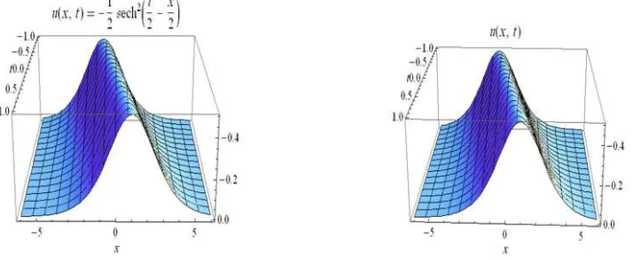
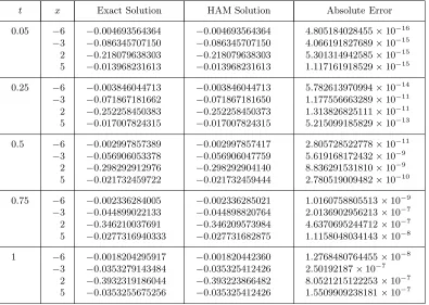
is convergence. In this case for −1 < t < 1 and ~ = −1, the exact soliton solution and HAM solution generated the same profile as are shown in Figure 2. The obtained numerical results for exact and HAM solutions are compared and summarized in Table 1. Clearly, from Table 1, this is shown to be in excellent agreement.
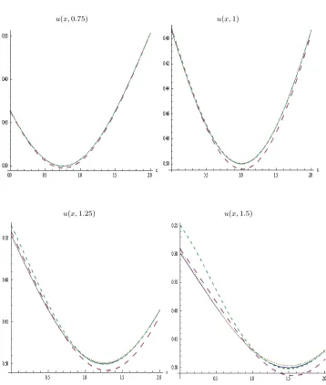
In Figure 3 we have MATHEMATICA graphs depicting u(x,0.75) u(x,1), u(x,1.25) and u(x,1.5) against x. The results obtained by the 8th-order approximation for ~ =
−0.5,−0.75,−1.We study the diagrams of the results obtained by HAM for ~=−0.5, ~= −0.75 and~=−1,and in comparison with the exact soliton solution (1) we conclude that the best value for~in this case is~=−1.
u(x,0.75) u(x,1)
u(x,1.25) u(x,1.5)
Table 1: Comparison of the HAM Solution with Exact Solution when ~ =−1 and t = 0, 0.25,0.5,0.75,1,Respectively
t x Exact Solution HAM Solution Absolute Error
0.05 −6
−3 2 5 −0.004693564364 −0.086345707150 −0.218079638303 −0.013968231613 −0.004693564364 −0.086345707150 −0.218079638303 −0.013968231613
4.805184028455×10⁻¹⁶ 4.066191827689×10⁻¹⁵ 5.301314942585×10⁻¹⁵ 1.117161918529×10⁻¹⁵
0.25 −6
−3 2 5 −0.003846044713 −0.071867181662 −0.252258450383 −0.017007824315 −0.003846044713 −0.071867181650 −0.252258450373 −0.017007824315
5.782613970994×10⁻¹⁴ 1.177556663289×10⁻¹¹ 1.313826825111×10⁻¹¹ 5.215099185829×10⁻¹³
0.5 −6
−3 2 5 −0.002997857389 −0.056906053378 −0.298292912976 −0.021732459722 −0.002997857417 −0.056906047759 −0.298292904140 −0.021732459444
2.805728522778×10⁻¹¹ 5.619168172432×10⁻⁹ 8.836291531810×10⁻⁹ 2.780519009482×10⁻¹⁰
0.75 −6
−3 2 5 −0.002336284005 −0.044899022133 −0.346210037691 −0.0277316940333 −0.002336285021 −0.044898820764 −0.346209573984 −0.027731682875
1.0160758805513×10⁻⁹ 2.0136902956213×10⁻⁷ 4.6370695244712×10⁻⁷ 1.1158048034143×10⁻⁸
1 −6
−3 2 5 −0.0018204295917 −0.0353279143484 −0.3932319186044 −0.0353255675256 −0.001820442360 −0.035325412426 −0.393223866482 −0.035325412426
5
Conclusion
In this paper, the homotopy analysis method (HAM) as proposed in [4, 5] is applied to obtain the solitary solution of the KdV equation. The resulted HAM solution at the eighth order approximation is then compared with that of the exact soliton solution of KdV equation, and it is shown to be in excellent agreement. Clearly, via the auxiliary parameter ~, HAM provides us with a convenient way to control the convergence of approximation series, which is a fundamental qualitative difference in analysis between HAM and other methods. Thus, we are of the opinion that this example enables us to show the flexibility and potential of the homotopy analysis method for solving other possible complicated nonlinear problems in industrial and engineering applications.
Acknowledgements
Mojtaba and Faisal are thankful to the Iranian and Sudanese governments for financial support respectively. This research is partially funded by the FRGS Vot No 78865 and RUG Vot: PY/2011/02329.
References
[1] Ablowitz, M. and Clarkson, P. Solitons, Nonlinear Evolution Equations and Inverse Scattering. Cambridge: Cambridge University Press. 1991.
[2] Drazin, P. G. and Johnson, R. S. Solitons: An Introduction. Cambridge: Cambridge University Press. 1996.
[3] Hirota, R. The Direct Method in Soliton Theory. Cambridge: Cambridge University Press. 2004.
[4] Liao, S. J. The Proposed Homotopy Analysis Technique for the Solution of Nonlinear Problems,Shanghai Jiao University: Ph.D. Thesis. 1992.
[5] Liao, S. J.Beyond Perturbation: Introduction to the Homotopy Analysis Method. Boca Raton, FL: Chapman and Hall. 2003.
[6] Liao, S. J. On the analytic solution of magnetohydrodynamic flows of non-Newtonian fluid over a streching sheet. J. Fluid Mech. 2003. 488: 189-212,
[7] Liao, S. J. A new branch of solution of boundary-layer flows over an impermeable stretched plate.Int. J. Heat Mass Transfer.2005. 48: 2529-39.
[8] Liao, S. J., Su, J. and Chwang, A.T. Series solution for a nonlinear model of combined convective and radiative cooling of a spherical body.Int. J. Heat Mass Transfer. 2006. 49: 2437-45.
[9] Liao, S. J. and Magyari, E. Exponentially decaying boundary layers as limiting case of families of algebrically decaying ones.Z. Angew. Math. Phys.2006. 57: 777-92.
[10] Liao, S. J. Series solution of unsteady boundary-layer flows over a stretching flat plate.
[11] Abbasbandy, S. The application of homotopy analysis method to nonlinear equations arising in heat transfer. Phys. Lett. A.2006. 360: 109-13.
[12] Abbasbandy, S. The application of homotopy analysis method to solve a generalized Hirota-Satsuma coupled Kdv equation.Phys. Lett. A 361.2007. 478-83.
[13] Abbasbandy, S. Homotopy analysis method for heat radiation equation.Int. Commun. Heat Mass.2007. 34: 380-87.
[14] Ayub, M., Rashed A. and Hayat, T. Exact flow of a third grade fluid past a porous plate using homotopy analysis method.Int. J. Eng. Sci.2003. 41: 2091-103.
[15] Hayat, T., Khan, M. and Ayub, M. Homotopy solutions for a generalized second-grade fluid past a porous plate.Nonlinear Dyn.2005. 42: 395-405.
[16] Hayat, T., Khan, M. and Ayub, M. On non-linear flows with slip boundary condition.
Z. Angew. Math. Phys.2005. 56: 1012-29.
[17] Asghar, S., Mudassar Gulzar, M. and Hayat, T. Rotating flow of a third grade fluid by homotopy analysis method. Appl. Math. Comput.2005. 165: 213-21.
[18] Sajid, M., Hayat, T. and Asghar, S. On the analytic solution of the steady flow of a fourth grade fluid.Phys. Lett. A.2006. 355: 18-26.
[19] Tan, Y. and Abbasbandy, S. Homotopy analysis method for quadratic Riccati differntial equation.Commun. Nonlinear Sci. Numer. Simul.2008. 13: 539-546.
[20] Abbasbandy, S. and Hayat, T. Solution of the MHD Falkner-Skan flow by homotopy analysis method.Commun. Nonlinear Sci. Numer. Simul.2009. 14: 3591-98.
[21] Wang, C., Wu, Y. and Wu, W. Solving the nonlinear periodic wave problems with the homotopy analysis method. Wave Motion.2005. 41: 329-337.
[22] Ablowitz, M and Segur, H.Solitons and the Inverse Scattering Transform. , Philadel-phia, PA: SIAM. 1981.
[23] Ablowitz, M and Clarkson, P.Soliton, Nonlinear Evolution Equation and Inverse Scat-tering. Cambridge: Cambridge University Press. 1991.
[24] Crighton, D. G. Applications of KdV.Acta Applicandae Mathematicae. 1995. 39: 39-67.