Characterization of Diffusion of Elastic Waves in Cortical Bone.

(1)

As bone ages, cortical bone replaces itself in a constant process of regeneration, responding to physical stresses on the skeleton to stimulate new bone formation. As people become less physically active or are subjected to extended periods of microgravity, the cellular structure of cortical bone may begin to exhibit anisotropy. This anisotropy leads to greater risk of fracture when stresses are applied. Current methods of measuring this imbalance require a CT scan and are fairly invasive. The use of multiple scattering in ultrasound presents a possible method for characterizing porosity and pore diameter in cortical bone. By measuring the properties of ultrasound diffusion in cortical bone in the proximal, distal, and central portions of the bone, we show a gradient in the porosity that could suggest a level of anisotropy. This method does not expose the patient to the radiation of a CT scan and in practice could theoretically be completed in a much shorter timeframe. Because it is non-invasive, it could be used repeatedly for monitoring bone loss with aging or during spaceflight.

In order to establish the relationship between diffusion constant, porosity, and pore size, 21 finite difference simulations of ultrasound propagation in bone were completed with varying micro-bone architectural parameters. These simulations spanned from 5 to 20 percent porosity, and pore sizes from 37 to 105 microns. The response of a slab of cortical bone to the transmission of a pulse is simulated, and the coherent backscattering signals are analyzed, allowing to estimate the diffusion constant in bone.

(2)

imaged with CT to provide exact regional porosity.

Simulation results show a fairly large correlation both between pore size to diffusion

constant and porosity to diffusion constant. In order to truly prove a result, there is most likely

the need for a denser sampling of the space.

Experimental results confirm the simulation: a distinct negative correlation between

porosity and diffusion constant was observed. These experiments need to be repeated on a

(3)

(4)

by

Mason R. Gardner

A thesis submitted to the Graduate Faculty of North Carolina State University

in partial fulfillment of the requirements for the degree of

Masters of Science in Mechanical Engineering

Mechanical and Aerospace Engineering

Raleigh, North Carolina

2016

APPROVED BY:

_______________________________ _______________________________

Dr. Marie Muller Dr. Fuh-Gwo Yuan

Committee Chair

(5)

DEDICATION

This work is dedicated to my mother and father, whose guidance has led me to be the man I

(6)

BIOGRAPHY

I am Mason Gardner, a current masters candidate at North Carolina State University.

Hailing from Chicago, Illinois, I spent most of my young life growing up and learning who I

was in nearby Chapel Hill. When not in the lab, which is rare the past few weeks, I play

professional ultimate Frisbee for the Charlotte Express of the AUDL. When not staying

active, I enjoy reading and watching sports, primarily soccer, American football, and

basketball. After graduation, I hope to obtain a job involving renewable energy or signal

(7)

LIST OF TABLES

(9)

LIST OF FIGURES

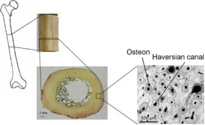
Figure 1.1-Acoustic microscopy scan of human cortical bone in the femur. ... 1

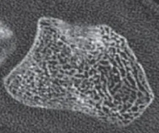
Figure 1.2-High Resolution CT scan of trabecular bone at 200um. ... 3

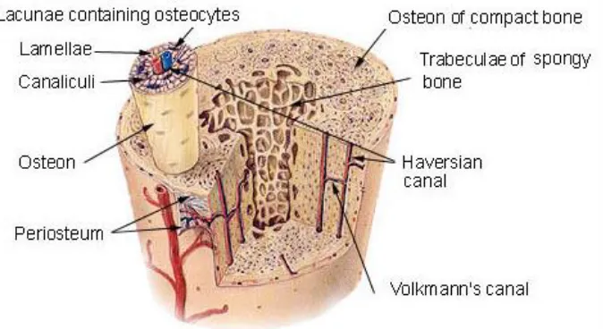
Figure 1.3- Structures of compact (cortical) human bone. ... 5

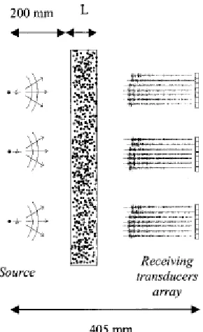
Figure 1.4- Experimental setup of Tourin11. ... 6

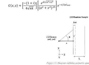
Figure 1.5- Diagram outlining geometric quantities in 2D experimentation. ... 8

Figure 1.7- Illustration of the coherent backscattering effect ... 9

Figure 1.6-Dynamic integration computes intensity over small time windows ΔT. ... 9

Figure 1.8- Right half of the coherent cone. Backscattering angle is the angle to the receiver normal to the surface of the sample. ... 11

Figure 1.9- Relation between enhancement factor and time window. The enhancement factor grows in time as multiple scattering becomes the dominant term. ... 12

Figure 2.1- Graphic representation of two impulse response requisitions for the first and last emitters. ... 13

Figure 2.2-Pore for .055mm diameter ... 15

Figure 2.3- Two simulation samples. ... 16

Figure 2.4- Total simulation area ... 17

Figure 5-Each color represents a receiver response before time shifting. ... 18

Figure 2.6-Image detailing 4 receiver responses after time shifting ... 19

Figure 2.7- Equidistant diagonals for averaging ... 20

Figure 2.8-Clean diaphysis, separated into distal, central, and proximal thirds. ... 21

Figure 2.9-Top view of central segment, with Lateral, Anterior Medial, and Posterior Medial sides labeled. ... 21

Figure 2.10-Image of experimental environment sans transducer for clarity. ... 22

Figure 2.11- Experimental setup top view ... 22

Figure 2.12. Normalized coherent cone in the far field. ... 23

Figure 2.1312-Near field normalized dynamic intensity illustrates the incoherent cone. ... 24

Figure 2.14-Coherent peak for a single time window. ... 25

Figure 2.15- Log-log representation of the narrowing coherent peak with time. ... 26

Figure 2.16-Results of diffusion constant measurements for constant pore size.. ... 27

Figure 2.17 - Relation between diffusion constant and pore size. ... 28

Figure 2.18- Coherent cone for the Anterior Medial Distal Image. ... 30

Figure 2.19 -Linear fit of the logwidth-logtime relationship. ... 31

Figure 2.20-MicroCT image scan of the distal posterior medial segment. ... 32

Figure 2.21- Binarized image of the distal posterior medial segment. ... 32

Figure 2.22 - Relation between average porosity of each bone segment and average diffusion constant. ... 33

(10)

CHAPTER 1

Introduction

In humans, bone growth is a cyclic process caused by responses to stress. Osteocytes

within the calcified bone matrix connect through the canaliculi of the bone to the surface,

signaling osteoblasts of the need for bone reinforcement. Shown in Figure 1.1[1]_{is an acoustic}

microscopy image of cortical bone. As can be seen in the image, human cortical bone is densely

packed, and healthy bone has a typical porosity of 5-10% [2]. The other main type of bone in

humans is trabecular or cancellous bone, which has a porosity in the range of 30% up to 90%

in some instances. Cortical bone is centered primarily in the diaphysis of the bone, while

trabecular bone resides on the ends of bones near joints. While monitoring trabecular health

(11)

can indicate instability in areas near a joint, monitoring cortical bone architecture can provide

an indicator to overal bone health throughout the body[2], and will be the focus of this study.

These osteocytes respond to regular mechanical loading on the bone in order to

stimulate bone growth, and thus the microstructure of bone is dependent upon stressing the

bone. While a simple stress like walking or lifting light weights can put the required stress on

the bones to maintain their full structural stability, these basic requirements are not always met.

While the predominant reason for bone loss is aging and a sedentary lifestyle, these losses can

also result from prolonged exposure to conditions in space[3]. Low amounts of gravitational

pull on the body in space reduce the stress placed on bones, and can lead to density loss of

almost 25% after only 6 months exposure[4]_{. If this pattern of inadequate bone renewal}

continues, this can lead to prolonged osteopenia or osteoporosis.

Osteopenia and Osteoporosis are the precursor and arrival of low density within the

bones of a human, respectively. This lower bone density leads to less structural stability in the

bone, meaning the affected human is more likely to suffer a fracture.

Currently the best gold standard for measuring this loss of bone density is through

dual-energy X-Ray absorptiometry, further referred to as DXA. This process works by emitting

x-ray particles at two energy levels, one targeting soft tissue and the other targeting calcium in

boney structures. Subtracting the soft tissue image from the boney image provides a clearer

resolution, at the tradeoff of greater radiation exposure. While this method is quite accurate in

(12)

provide information specific to the micro-architecture of the bone. In addition, DXA can in

some instances provide swayed results based on high fat content in the area of the scan [5,6].

In order to receive information on the microarchitecture of the bone, a high resolution

CT scan is the next option. High resolution CT imaging is performed by computer processing

of several scans taken in a circular path around the object of interest, providing a three

dimensional image of the structure. High resolution CT is capable of pixel sizes on the order

of 100-300µm. An image of trabecular bone is shown in figure 1.2[7]_{. While this resolution is}

generally acceptable for trabecular bone, the smaller architecture within cortical bone is still

not fully distinguishable directly. HrCT also poses an exposure to many x-rays at one period,

meaning significant exposure to radiation. This radiation puts a limit on the frequency of bone

scans, due to limitations on patient exposure levels.

The use of backscattering ultrasound seeks to eliminate the issues with DXA and CT

scanning. Conventional ultrasound imaging generally seeks to avoid bone. With its

complicated microstructure, signals received from bone often appear noisy, or segmented. This

study attempts to use ultrasound to obtain signals scattered through cortical bone

(13)

architecture. These reverberated signals contain information about how the signal diffuses

within the bone, and can offer a better estimation of localized bone density loss. This means

that with proper implementation this technology could be used to identify fracture risk,

allowing for analysis of specific movement patterns that might endanger the patient.

Currently, quantitative ultrasound is used primarily at bony sites where the region of

interest is close to the skin. Measurements are often taken at the heel due to low amounts of

soft tissue interference, though a more localized technique would be expected to be far superior

for something like hip fracture risk[1]. Advances in computer modeling allow for better

understanding of the actual path ultrasound takes through such a complicated structure as bone,

and these advancements are making it easier to push the boundaries of implementing

ultrasound in areas previously thought too noisy for trustworthy results.

Greater knowledge of the rate of bone loss can allow for individualized workout plans

or supplementation in order to restore healthy bone functionality, while offering flexibility in

catering these therapies for best results. Fast, noninvasive ultrasound testing could make bone

density screening quite simple, taking only several minutes and allowing for early recognition

of bone loss, which is in general not reversible. The lack of radiative exposure also means that

at-risk individuals could receive testing very regularly to monitor bone density and better

identify the habits that are causing bone loss.

Previous Research

Multiple scattering for wave forms has been studied extensively both for electron

(14)

scatterers are the micro-architectural structures pictured in figure 1.3[8]. The majority of

scattering events occur at lacunae and Haversian canals.

As a wave propagates through a medium of randomly placed scatterers, the wave may

exhibit one of two regimes. The first regime is the coherent regime. This regime is

characterized by a wave that maintains its initial direction even after averaging over all possible

scatterer placements. After several scattering events, a diffusive regime can be observed in the

form of a diffusive halo which outlines the slow dispersal of the wave amongst the forest of

scatterers.

In order to understand the statistical distribution of these waves over time in a multiply

scattering medium, it is easiest to visualize the path of a single particle. Using classical

diffusion, the probability of finding the particle at any particular point in space as a function

of its distance from the emitter in two dimensions can be expressed using[9]

𝑝(𝑟, 𝑡) = 1

4𝜋𝐷𝑡exp⁡[−

𝑟2

4𝐷𝑡]

(15)

in which D is the diffusion constant of the material-wave pairing, r is the linear distance from

the emitter, and t is the time since emission. As the particle passes through a random medium

such as the small channels of cortical bone, diffusion of this particle can be viewed as taking a

random path from the emission point back to the emitter. Statistically, the inverse path is

equally likely and exactly in phase. As a results, both interfere constructively and there is a

distinct peak in the normal probabilistic wave distribution centered about the emitting point.

This reciprocity means that the probability is twice as large as the classical case, yielding a

factor of 1/2πDt. The greater probability of remaining near the original emitter is referred to

as weak localization[10].

Figure 1.4- Experimental setup of Tourin11_{. This test is}

(16)

Tourin et al[11] use a linear transducer array to insonify a sample created from randomly

placed cylindrical steel rods as shown schematically in figure 1.4. Each signal transmitted

through the sample is composed of a ballistic and forward scattered wave, both of which are a

function of the sparse distribution of scatterers within the sample. As is to be expected, initial

testing suggests that both overall signal amplitude and coherent wave amplitude become less

visible in through transmission as sample width increases. In noticing this, Tourin suggests the

use of the average intensity within the medium in order to make estimates of the average

architectural parameters. This method is dependent on ergodicity, and a sufficiently thick

sample, or more importantly upon a sufficiently large number of scatterers. Once the sample

is thick enough to restrict the beam to the diffusive regime, then an ensemble average over the

length of the sample allows for calculation of both mean free path, l, and the diffusion constant,

D, which measures the rate of growth of the diffusive halo during its random walk through the

medium.

The diffusion of the wave within a sufficiently thick medium given as a function of

intensity is[9]

(𝐷∆ − 𝛿

𝛿𝑡) 〈𝐼(𝑟, 𝑟′, 𝑡, 𝑡′)〉 = 𝛿(𝑟 − 𝑟′)𝛿(𝑡 − 𝑡′)

where D is the diffusion constant, I is the intensity Green function, and r and t are instantaneous

position and time. This theory has applications in optics, and is often referred to as the ‘plane

wave’ approach, due to the plane-like semblance of the wave in the far field. In 2D free space,

(17)

𝐺(𝑅) ≈ − [(1 + 𝑖) 4√𝜋𝑘𝑅] 𝑒

𝑖𝑘𝑅

with k the wave vector and R the Euclidean distance from the emitter. Once the signal enters

the sample, though, this approximation is no longer valid, and instead is defined as[9]

𝐺(𝑥, 𝑧) ≈ [−(1 + 𝑖) 4√𝜋𝑘 ] [

𝑒𝑖𝑘√𝑎2_+𝑧2

(𝑎2_{+ 𝑥}2₎.25] 𝑒−𝑧/2𝜇𝑙𝑒𝑥𝑡

With µ = cosθ, lext the extinction length into the sample, a, the length to the samplesurface, z,

the distance parallel to the 2D surface, and θ the angle with the vertical as shown in figure 1.5.

It is from these two parameters that we hope to characterize cortical bone porosity and

pore size, albeit in a medium that is the inverse of the sample from Tourin[11]_{depicted in figure}

1.4.

(18)

In the present work, we chose to work on the backscattered signals instead of the

through transmitted signals, because through transmission is impractical in vivo in bone.

Calculation of the transport mean free path, defined as the mean distance traveled between

consecutive particle collisions, may be performed through integration of the intensity of

Figure 1.7- Illustration of the coherent backscattering effect, showing that a path and its reciprocal path have the same likelihood and are resistant to averaging due to this reciprocity. Figure 1.6-Dynamic integration computes

intensity over small time windows ΔT.

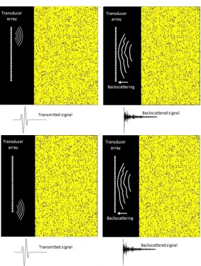
Impulse Response Matrix

In order to obtain the Green function of the array-bone sample pairing, we used the

ultrasound sequence described as follows, further referred to as the Impulse Response

Matrix: One by one, each of the elements of a linear transducer array transmits a short

pulse. For every transmission, the field backscattered by the pores is measured on the

whole array. The resulting signals constitute a temporal and spatial sampling of the

backscattered wave field. Once this is repeated for all of the elements, the impulse

(19)

dynamic time windows (Fig 1.6)[11], allowing for analysis of the coherently backscattered peak

with time. This dynamic windowing is performed on the impulse response matrix. The signal

received resembles a single coherent peak, meaning that it is resistant to averaging of the

medium, and is present because of the reciprocity of the medium- that is to say, signal from

emitter x scattered through the medium to receiver y has the same phase and path as the signal

that travels through the medium from y to x. This principle is shown in figure 1.7 from

Akkermans et al10.

Instead of integration over the whole signal intensity, the dynamic case simply chooses

a small time window- ideally a window of time that will on average capture only a single

scattering event. The problem then lies in the fact that there must be some a priori knowledge

of the structure for testing in order to find an effective window. Thus, it is required that there

be at least a ballpark estimate of the distance between scatterers, from which an average

scattering time can be calculated by dividing by the wave speed in bone. While estimations of

cortical bone structure in humans are fairly easy and reasonable to make, the presence of

drastically different structures such as fractures may cause errors in the final measurement in

the dynamic case.

In making calculations with the intensity of the backscattered signal, another method

is to calculate an enhancement factor as performed by Ishimaru[12]. If the first order

backscattering intensity is given as I1, the ratio of the amplitudes can be given as

𝐼₁+ 𝐼_𝑚𝑙 + 𝐼_𝑚𝑐

𝐼1+ 𝐼𝑚𝑙 =

(20)

where Imlis the ladder term, representing the incoherent wave, which is the wave traveling in

the diffusive regime, and Imc is the maximally crossed term, and represents the coherent wave.

In calculation of the enhancement factor and calculations resulting from it, there is the

assumption that the coherent and incoherent waves have the same intensity, allowing the

simplification shown above. The final ratio above provides the enhancement factor, a value

between 1 and 2, which can be used to estimate mean free path. As described by Derode[13] et

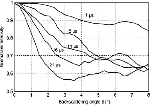
al, this method involves first creating the backscattering cone. This is done by integrating the

signal intensities over 2-µs intervals from an impulse response matrix just as in Tourin7. Then,

he plots the average intensity of each emitter-receiver angle for each time window, forming

the peak shown in figure 1.8. Derode then chooses an angle with respect to the emitter at which

the coherent peak ends and the peak resolves to noise. He then approximates the enhancement

factor using

(21)

𝐸𝐹 = 𝐼(0, 𝑡) 𝐼(𝜃_𝑚𝑎𝑥, 𝑡)=

𝑆𝑆(0, 𝑡) + 𝑀𝑆(0, 𝑡) 𝑆𝑆(0, 𝑡) + 0.5𝑀𝑆(0, 𝑡)

where MS and SS denote the multiple and single scattering respectively. This version of the

enhancement factor formula has half the contribution from multiple scattering in both the

denominator and numerator compared with Ishimura’s relation, but assuming that multiple

scattering dominates the single scattering, the two equations approach equality as shown below

𝑆𝑆(0, 𝑡) + 𝑀𝑆(0, 𝑡)

𝑆𝑆(0, 𝑡) + 0.5𝑀𝑆(0, 𝑡)≈

2𝑀𝑆(0, 𝑡)

𝑀𝑆(0, 𝑡) ≈

𝐼₁+ 2𝐼_𝑚𝑙 𝐼1+ 𝐼𝑚𝑙

where the MS and SS denote single and multiple scattering respectively in Derode’s

convention, and I1and Iml are the single and multiple scattering in Ishimura’s definition.

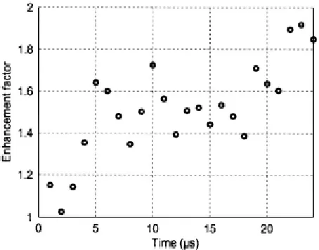
Derode then continues by plotting each value of the enhancement factor with its

respective time interval, as shown in figure 1.9. From the Derode’s definition of enhancement

factor, when multiple and single scattering are equal, the enhancement factor becomes 4/3,

which he uses in his EF plot to identify a typical time, τ. Multiplying the typical time by the

(22)

wave speed in the medium gives an upper bound on the mean free path. While this method is

simple and one of the few methods than can fully sidestep absorption, the value of 4/3 is

extremely arbitrary. This method is also quite sensitive to the point chosen as the end of the

coherent peak. The choice of this point can drastically effect the results, even after averaging

over several realizations.

(23)

Chapter 2

Simulation Methods

Testing was performed both in simulation as well as on bovine tibial cortical bone.

Simulations were performed using SimSonic finite difference finite time software[14], which is

open source and available online. Each simulation consists of a 2D map, through which a

single wavelength 8 MHz signal was transmitted. The receiver array is placed normal to the

surface of the sample in each case, and no apodization was used. Each map was 9mm long and

15mm deep, in order to ensure that the signal entering the sample did not permeate completely

to any significant extent. In order to obtain the impulse response matrix, a single transducer

would emit, and then all would receive, and this would be repeated as shown in figure 2.1.

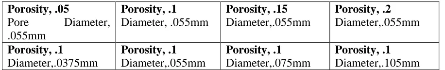
The maps used had a porosity and pore size as shown in table 2.1.

Table 2.1

Porosity, .05

Pore Diameter,

.055mm Porosity, .1 Diameter, .055mm Porosity, .15 Diameter,.055mm Porosity, .2 Diameter,.055mm Porosity, .1 Diameter,.0375mm Porosity, .1 Diameter,.055mm Porosity, .1 Diameter,.075mm Porosity, .1 Diameter,.105mm

Table 2.1. Layout of sample parameters for simulations performed. Three of each set of parameters was performed in order to allow for averaging.

Each map was generated through monte carlo placement of pores repeated until the desired

porosity had been reached. For each set of parameters, three maps were generated. The

intensity responses of these three maps would be averaged together in order to mimic an

ensemble averaging and produce the coherent peak. This also ensured that there would be no

(24)

Due to size constraints for the entire simulation matrix, a resolution of .005mm was

chosen. While this resolution allowed for a simulation over a couple days as opposed to several

weeks, the larger resolution meant a slightly inferior approximation at a truly circular shape,

as is shown in figure 2.2. Since the grid step was chosen, the time step became subject to the

Courant-Friedrichs-Levy (CFL) condition, which relates grid step and time step by

∆𝑡 ≤ 1

√𝑑∙ ∆𝑥 𝑐_𝑚𝑎𝑥

where d is the number of dimensions for the simulation (in this case 2), and cmax is the

maximum wave velocity at any point in the simulation. The value for maximum wave velocity

was the ultrasound wave velocity within cortical bone in this simulation, which is set to 4

mm/µs. Using these values, and allowing a slight tolerance away from the maximum time step,

a value of .875 ns was used in all simulations.

(25)

By holding pore size constant over a range of porositys and the reverse, we hope to be

able to establish a relationship between average pore size, porosity, and diffusion constant or

mean free path. For each mapping configuration, 3 different maps were created, a pair of which

are shown in figure 2.3, allowing for averaging of responses. This resembles the ensemble

averaging performed by Tourin[11]_{, in that each map is sufficiently different enough that a}

single emitter-receiver pairing does not encounter the same exact medium but still sees the

same overall material aspects. Testing was also performed both in the near-field and far-field,

in order to test variability in responses and in order to mimic testing in vitro at both bony

surfaces and bones that are covered by a layer of tissue.

(26)

Each of these maps was then ‘immersed’ in water as shown in figure 2.4. The total

matrix insonified was then 10mm wide by 40 mm deep. The transmitter was placed at the left

furthest end, 17.5mm away from the sample in order to ensure that each measurement was in

the far field. Each simulation ran for a time, t, of 48μs, allowing the signal sufficient time to

reach the sample, reverberate, and return to the emitting array. The emitting array was

simulated as 32 transducers each .3mm wide. Each in turn would emit an 8 MHz signal into

the map. With that single element on the array acting as the emitter, the received signal was

recorded on all 32 elements. This was repeated until every element had acted as an emitter,

rendering a n by n emitter-receiver matrix here on referred to as the impulse response matrix,

where n is the 32 elements of this array.

(27)

For each signal in the impulse response matrix, the initial 2000 time points were cut in

order to eliminate cross talk between emitters. This cuts the first 1.75 μs from the

signals-drastically below the amount of time for any signal to have returned to the array. Figure 2.5

shows the responses before time shifting after emitting from a single element. From this figure

it is clear to see that the individual receivers, each colored differently, return with a slight delay.

This is due to the greater distance traveled as the signal is received on receivers further from

the emitter. To combat this delay, each signal was time shifted such that every received signal

had the same arrival time. Very low noise levels in simulation allowed for this time shift to be

completed by finding the first point just above the noise level and removing signal prior to that

(28)

threshold value. After time shift, the responses to a single emitted signal look more like figure

2.6.

From the impulse response, each signal was segmented into tw=.5µs windows and the

intensity was calculated by summing the intensity within that window (Refer to Fig. 1.6). Next,

the intensity for each time window was averaged over each respective emitter-receiver

distance, i.e. the average intensity was computed for the first time window for every iteration

of the receiver being 1 pitch length left of the emitter, then 2 pitch lengths left, etc. The pattern

(29)

of averaging within this matrix is shown in figure 2.7. Each color of diagonal represents a

separation distance between the receiver and emitter. Averaging the intensity at each ‘color’

yields a (2n-1) vector of average intensities for each distance from the emitter. This is the first

ensemble average. The vector is then normalized to 1 by dividing the vector by its maximum.

The averaging pattern in figure 2.7 is repeated for each time window and concatenated

together, yielding a matrix of size (2n-1) x (# of time windows). This matrix is the response of

a single simulation, and the average of 3 simulations is analogous to a full ensemble averaging

that finally yields the coherent cone.

(30)

Experimental Methods

The process for experimentation was designed in order to maintain similarity with the

simulations. Experiments were performed on bovine cortical bone from the tibia, due to its size

and relatively flat shape. A clean diaphysis is shown in figure 2.8. These bone samples were

each obtained from adult cows, though age and lifestyle were unknown. After thawing, each

bone was submerged in soap and water until any flesh remaining on the bone could be stripped

with a knife. Special attention was paid to drying the bone before any freezing so as to

minimize cracks caused by ice formation. The diaphysis was then portioned into thirds, and

the sections labeled as proximal, central, and distal as in figure 2.9. Testing was then performed

on the lateral, anterior medial, and posterior medial sides of each segment. These segments

were chosen for the relatively flat face along which testing could be performed. Measurements

were performed using an L11-4v Verasonics 128 element array with a central frequency of 7.8

MHz. Each bone segment was submerged in water and suspended atop a beaker, as shown in

figures 2.10 and 2.11, minimizing any signal reflected from other surfaces during testing. Each

Figure 2.8-Top view of central segment, with Lateral, L, Anterior Medial, AM, and Posterior Medial, PM sides labeled.

(31)

stage of testing consisted of 4 measurements made on each side of the bone segment, once

again by emitting with a single transducer and receiving with the entire array. These signals

were recorded using the Verasonics system, which works in conjunction with MATLAB to

save and modify the data.

Each of the four measurements was taken after slight adjustment of the sample, in order

to decouple any single emitter from a specific area of the bone. This gave a total of 36

measurements in 9 positions on the bone. For these measurements, the array was placed

perpendicular to the grain of the bone and normal to the surface of the bone.

Figure 2.10-Image of experimental environment sans transducer for clarity. Pictured is the anterior medial side of the distal segment.

(32)

Once the gambit of readings was completed, the following step was processing similar

to the processing performed for each simulation. After eliminating cross-talk between elements

of the array by severing the first hundred time points of each measurement. Signals were again

concatenated into a 32 by 32 matrix of signals.

Simulation Results

The coherent backscattering cone provides an image of the intensity of the signal as it

propagates in time, as shown in figure 2.12.

Figure 2.12. Normalized coherent cone in the far field. The large initial intensity is the result of the ballistic wave, which is signal that has not permeated the sample. As time increases, the signal becomes much weaker and begins to dissolve into noise.

For the far field instance, there is a very wide initial amplitude received, which is the

ballistic wave. This is the very first portion of the signal received, which has not penetrated the

sample and simply reflected off the sample surface. The coherent peak then narrows at a rate

(33)

of _√𝐷𝑡1 as predicted in Tourin[9]. It is important to note that this narrowing of the coherent peak

may only occur in far field measurements, as the emitted wave in the near field does not reach

the sample in a way that the plane-wave approximation is valid, preventing the reflection of a

ballistic signal.

Purely for reference, in the near field image it is much clearer to see the incoherent

growth of the signal as in Figure X. Initially, only transducers close to the emitter receive any

notable amplitude. As time progresses though, wave paths that have been multiply scattered

begin to reach further displaced receivers, as shown by the widening of the intensity band. This

incoherent growth is the maximally crossed term in Ishimura’s enhancement factor[12].

(34)

Simulations and experimental testing were both carried out in the far field in order to

study specifically the diffusion constant as it is derived from the coherent peak diminishing.

For each set of parameters, the first step was to calculate the normalized dynamic intensity

profile, by averaging intensities equidistant from the emitter as in figure 2.7 for each time

window. To repeat, this first averaging is the first step to an ensemble average. The normalized

dynamic intensity profile was averaged over three simulations, in order to form a full ensemble

average. After averaging, the next step was to fit the coherent peak with a Gaussian curve.

This was done iteratively for each time window in the dynamic intensity matrix. Once the

standard deviation for each Gaussian fit was stored, these standard deviations were then used

to calculate the full width at half maximum via the equation (derivation in Appendix A),

𝛿 = 2√2 ln 2 𝜎 = 2.355𝜎

(35)

where δ is the full width shown in figure 2.14 at half maximum and σ is the standard deviation.

The natural logarithm of the widths was then plotted against the natural logarithm of each time

window, as shown in figure 2.15.

While the coherent peak contains an ensemble average of only three measurements, there is

still a fairly noticeable negative correlation in the data as could be predicted. A linear fit of

these points provides an estimate of the log-width intercept. From this intercept, the diffusion

constant may be found through the equation

ln 𝛿 = 1.12 1

𝑘√𝐷 ln 𝑡⁡

where k is the wavenumber of the emitted wave. Along with each linear fit, the 95%

confidence interval of each intercept calculation was stored in order to provide a level of

(36)

uncertainty in each measurement. The results of the diffusion constant measurements for the

individual porosities but same pore size are shown in figure 2.16.

This process was repeated for simulations in which the porosity remained a constant

10%, while the pore sizes were adjusted between 105micron and 35 micron. The results are

shown in figure 2.17.

(37)

Both of figures 2.16 and 2.17 provide important information regarding the path of the

signal within the bone. The linear relation between porosity and diffusion constant suggests

exactly as one might expect- that if the pores are all of the same size, the number of scattering

events will increase proportionally to the number of scatterers in the sample being tested. In

contrast, the relation between the diffusion constant and pore size appears to exhibit

diminishing returns. This is most likely due to the fact that as the size of the pores becomes

(38)

larger, the number of pores required to reach 10% porosity varies inversely with the pore size,

as illustrated in table 2.2.

While the diminishing returns as average pore size increases are something to keep in

mind, it is important to note that the diffusion constant values are still differentiable up to pore

sizes around 105 microns. This value can actually be improved with further ensemble

averaging, which is expected to increase the linearity before fitting. A greater fit would lead to

a narrower error bar, and allow for more precise readings. With that in mind, it is also pertinent

to note that the average cortical bone pore size[17] is generally in the range of 10µm-50µm and

therefore well below sizes at which the statistic begins to lose resolution.

Pore Size (mm) Number of Pores for 10% Porosity

Change in

Number of Pores

.035 18621 NA

.055 6667 -11954

.075 3625 -3042

.105 1704 -1921

.125 1225 -479

.145 881 -344

.165 678 -203

.185 536 -142

(39)

Experimental Results

The experimental results showed patterns similar to those found in the simulation

results. As in the simulations, the impulse response matrix was acquired using short pulses

with an 8 MHz central frequency. Shown in Figure 2.18, the coherent cone still has a relatively

similar appearance, although appearing sparser at the initial several time windows. Once again,

like the simulations, this dynamic intensity profile was averaged with another to form an

ensemble average and bring the coherent cone more into focus.

For each of the 9 imaging locations, the width of the cone was measured just as in

simulation and a log-log plot of the width with time was assembled as in Figure 2.15. The

initial 3µs were omitted from the fit in order to ensure a fit similar to simulation. From this fit

(40)

an intercept, ln δ, was calculated along with an uncertainty in that estimation. Then, the

equation

ln 𝛿 = 1.12 1

𝑘√𝐷 ln 𝑡⁡

was used in order to solve for the diffusion constant. In dealing with the experimental data, the

only major changes made to the preparation of the data was that fewer time windows were

used in making the fit. Referring back to figure 2.18, it can be seen that the cone narrows as in

the simulations, but at a point around 14 time windows once again widens. This is most likely

due to the second round trip made by the ultrasonic pulse. Thus, time points just before this

second widening were removed.

In order to check the accuracy of these estimates, the bone samples were also cut into

1cm x 6mm x 6mm rectangular prisms and microCT scanned with a pixel resolution of 6µm

(41)

and a slab width of 12µm. The Biomedical Research Imaging Center of the University of North

Carolina at Chapel Hill offers access to micro-CT scanners. For this project, we used the

SCANCO µCT 40 scanner, a high resolution desktop cone-bean X-ray scanner with a top

resolution of 6 µm. The software associated to the scanner offers complete image

reconstruction. One of the scan slices is shown in figure 2.20. These images were filtered using

a 3D median filter, binarized, as shown in figure 2.21 and then used to calculate an average

porosity for the sample region. The level of filtering and binarizing limit were judged based on

output resembling cortical bone in cows. Items smaller than 49 connected pixels were deemed

noise and changed to bone. The porosities found through this method were in the range of

2-5%, which is somewhat below the 5-30% estimate cited by Carter et al2.

Two of the measurements of the diffusion constant were thrown out due to poorness of

fit that resulted in error several orders of magnitude larger than the measurements.

Figure 2.20-MicroCT image scan of the distal posterior medial segment.

(42)

If we are to average the values obtained for each segment and the average segment

porosity, a pattern emerges. This pattern can be seen in figure 2.22.

In the figure, there is still a slight negative trend, with what appears to be a problem of

resolution between the proximal and distal segments. It is also particularly encouraging that

the central portion of bone- which is furthest from the trabecular regions and has the lowest

porosity- also had the highest diffusion constant as the simulations would have predicted. That

being said the data is also fairly sparse due to the small sample size after averaging.

Figure 2.22 - Relation between average porosity of each bone segment and average diffusion constant. The high diffusion constant in the lowest porosity region mimics the negative trend from simulations.

Distal

Central

(43)

Chapter 3

Conclusion

To conclude, this study sought to establish a concrete relationship between porosity,

pore size, and the rate of ultrasound diffusion in cortical bone using 8 MHz ultrasound pulses.

Data both in simulation and in experimental testing was accumulated in an impulse response

matrix, in which iteratively a single transducer emits a pulse which is backscattered by the

sample and collected on the whole array. This is repeated for all emitters and concatenated into

a square array of emitters and receivers. By averaging windowed intensities over discrete

distances from the emitter, a dynamic intensity profile is created. An ensemble average of this

intensity profile provides the coherent cone, from which the diffusion constant may be

estimated.

When this process was applied to simulations, there returned a distinct pattern both

between porosity and diffusion constant as well as pore size and diffusion constant. This study

suggests that diffusion rate and porosity are negatively linearly correlated. Pore diameter and

diffusion constant appear to be positively correlated, although their relationship appears to be

higher order.

Application to testing in real bone presented a differing set of issues from those of the

simulations. First and foremost was simply a greater level of noise and reflections which were

not present in simulation. Even with these issues, there appeared still the same correlation

(44)

Perspectives

In order for a technique built off of this methodology to reach in vivo application, there

are a number of minor tweaks that might be made. Most likely, because of the confounding

effect that pore size and porosity have on the diffusion constant, more research might have to

go into the direct relationship between diffusion constant and yield strain. While it would be

nice to determine the exact microstructure of each patient, ultimately the goal of this project is

to make a cheaper, less invasive way of testing bone stability. A study on human bone is

required, including both healthy and osteoporotic bone, on which mechanical testing would be

performed, additionally to ultrasound testing. The diffusion constant would then be compared

to the yield strain. A large number of saomples will be required to ensure statistical validity.

In vivo application of this technique would require a relatively flat bony surface on

which to test such as the anterior tibia in humans. With application of ultrasound gel or an

acoustic stand off pad, there would be proper separation between the array and bone surface to

make purely far field measurements. Three testing locations at the top, middle, and bottom of

the tibia could be used, each time making 10-20 impulse measurements that could be used to

Figure 3.1- Collimated beam focused at a+zr/2. This focusing

(45)

form a very precise ensemble average. This region of bone is close to the skin, minimizing any

influence from soft tissue. Another approach to studying diffusion constant will be imaging in

the near field. Aubry et al[18] make use of Gaussian beamforming, as shown in figure 3.1 to

focus an ultrasound beam in a small region. The resulting impulse matrix then would offer an

estimate of the local diffusion constant, allowing for measurement of structural instability in

areas of the bone already established as weak points. These spots might include previous

(46)

REFERENCES

[1] Laugier, Pascal, and Guillaume Haïat. Bone Quantitative Ultrasound. Dordrecht:

Springer, 2011. Print.

[2] Carter, Dennis R., and Wilson C. Hayes. Journal of Bone and Joint Surgery 59.7 (1977):

954-62. Web. 6 June 2016.

[3] Vico, Laurence, Philippe Collet, Alain Guignandon, Marie-Hélène Lafage-Proust,

Thierry Thomas, Mohamed Rehailia, and Christian Alexandre. "Effects of Long-term

Microgravity Exposure on Cancellous and Cortical Weight-bearing Bones of

Cosmonauts." The Lancet 355.9215 (2000): 1607-611. Web. 6 June 2016.

[4] Rittweger, Jorn, and Petra Frings-Meuthen. "Bone Loss in Microgravity."ResearchGate.

Physiology News, Autumn 2013. Web. 27 June 2016.

[5] "Dual Energy X Ray Absorptiometry - Bone Mineral Densitometry." Radiation

Protection of Patients. International Atomic Energy Agency, 2013. Web. 27 June 2016.

[6] "Dual Energy X-Ray Absorptiometry Procedures Manual." National Health and Nutrition

Examination Survey (n.d.): n. pag. CDC.gov. National Center for Health Statistics, 19 Feb.

2016. Web. 20 June 2016.

[7] Genant, H. K., K. Engelke, and S. Prevrhal. "Result Filters." National Center for

Biotechnology Information. U.S. National Library of Medicine, n.d. Web. 20 June 2016.

[8] M, David. Compact Bone and Spongy (Cancellous Bone). Digital image.These Bones of

(47)

[9] Tourin, Arnaud, Arnaud Derode, Philippe Roux, Bart A. Van Tiggelen, and Mathias Fink.

"Time-Dependent Coherent Backscattering of Acoustic Waves." Phys. Rev. Lett. Physical

Review Letters 79.19 (1997): 3637-639. Web. 8 Aug. 2015.

[10] Akkermans, E., P. E. Wolf, and R. Maynard. "Coherent Backscattering of Light by

Disordered Media: Analysis of the Peak Line Shape." Phys. Rev. Lett. Physical Review

Letters 56.14 (1986): 1471-474. Web. 7 June 2016.

[11] Tourin, Arnaud, Arnaud Derode, Aymeric Peyre, and Mathias Fink. "Transport

parameters for an ultrasonic pulsed wave propagatingin a multiple scattering

medium" National Center for Biotechnology Information. U.S. National Library of Medicine,

4 Apr. 2000. Web. 27 June 2016.

[12] Yamato, Yu, Hideo Kataoka, Mami Matsukawa, Kaoru Yamazaki, Takahiko Otani, and

Akira Nagano. "Distribution of Longitudinal Wave Velocities in Bovine Cortical Bone in

Vitro." Jpn. J. Appl. Phys. Japanese Journal of Applied Physics 44.6B (2005): 4622-624.

Web. 15 Mar. 2016.

[13] Bergmann, Gerd. "Physical Interpretation of Weak Localization: A Time-of-flight

Experiment with Conduction Electrons." Phys. Rev. B Physical Review B 28.6 (1983):

2914-920. Web. 20 June 2016.

[14] Ishimaru, A. "Wave Propagation and Scattering in Random Media and Rough

Surfaces." Proceedings of the IEEE Proc. IEEE 79.10 (1991): 1359-366. Web. 20 June 2016.

[15] Bossy, Emmanuel. SimSonic. SimSonic-FDTD Simulation of Ultrasound Propagation.

(48)

[16] Derode, Arnaud, Victor Mamou, Frederic Padilla, Frederic Jenson, and Pascal Laugier.

"Dynamic Coherent Backscattering in a Heterogeneous Absorbing Medium: Application to

Human Trabecular Bone Characterization." Dynamic Coherent Backscattering in a

Heterogeneous Absorbing Medium: Application to Human Trabecular Bone

Characterization. Applied Physics Letters, 7 Sept. 2005. Web. 10 Jan. 2016.

[17] Lee, Steve, Michael Porter, Scott Wasko, Grace Lau, Po-Yu Chen, Ekaterina E.

Novitskaya, Antoni P. Tomsia, Adah Almutairi, Marc A. Meyers, and Joanna Mckittrick.

"Potential Bone Replacement Materials Prepared by Two Methods." MRS Proc. MRS

Proceedings 1418 (2012): n. pag. Web. 25 June 2016.

[18] Aubry, Alexandre, and Arnaud Derode. "Ultrasonic Imaging of Highly Scattering Media

from Local Measurements of the Diffusion Constant: Separation of Coherent and Incoherent

(49)

(50)

1-

𝑒

−(𝑥0−𝜇)

2

2𝜎2 = 1 2

−(𝑥0− 𝜇)

2

2𝜎2 = − ln 2

(𝑥₀− 𝜇)2 _{= 2𝜎}2_{ln 2}