Bayesian Inference Under Shape Constraints.

(1)

ABSTRACT

CHAKRABORTY, MOUMITA. Bayesian Inference Under Shape Constraints. (Under the direction of Subhashis Ghosal).

In the context of nonparametric univariate monotone regression with unknown error varianceσ2_{, we study global posterior contraction rates and the point-wise coverage of a}

Bayesian credible interval. Using a finite random series of piece-wise constant functions with normal basis coefficients as a prior for a regression function f, we obtain a conjugate posterior and project each sample from the unrestricted posterior on the shape-constrained space of functions, inducing a distribution to be called the “projection-posterior". For global contraction rates, point estimation and credible sets, a lot more tractability is obtained by considering this projection-posterior distribution. We show that the projection-posterior contracts at the minimax raten−1/3_{with respect to the}_L

1-distance, and also with respect to

the empiricalLp-distances up to a logarithmic factor. For the limiting coverage of a credible

interval off evaluated at a fixed pointx0, we observe a very interesting phenomenon that the

coverage may be higher than the nominal credibility level, the opposite of a phenomenon observed by Cox (1993) in the context of smooth nonparametric signal estimation. We then show that a re-calibration technique can give the right coverage. By employing the distance of the unrestricted posterior from its projection on the monotone class, we develop an asymptotically optimal Bayesian test for the hypothesis of monotonicity. Using the idea of enlarging the region near the null hypothesis off being in the monotone class, as proposed by Salomond (2018), we construct a universally consistent Bayesian test for monotonicity with optimal power properties.

For a monotone decreasing probability density on the positive real line, we study global posterior contraction rates and the point-wise coverage of a Bayesian credible interval. Using a random histogram with Dirichlet basis coefficients as a prior for a densityg, we obtain a conjugate posterior and use the projection-based approach to project each sample from the unrestricted posterior on the space of monotone decreasing densities. We show that the projection-posterior contracts at the minimax raten−1/3_{with respect to the}_L1

-distance forg on a bounded domain, and the minimax rate up to a logarithmic factor forg on an unbounded domain. Forg evaluated at a fixed point, we obtain a projection-posterior credible interval with the asymptotic coverage more than the credibility level, a phenomenon similar to that observed in the case of monotone regression.

(2)

(3)

(4)

Bayesian Inference Under Shape Constraints

by

Moumita Chakraborty

A dissertation submitted to the Graduate Faculty of North Carolina State University

in partial fulfillment of the requirements for the Degree of

Doctor of Philosophy

Statistics

Raleigh, North Carolina 2019

APPROVED BY:

Soumendra Lahiri Ryan Martin

Sujit Ghosh Subhashis Ghosal

(5)

BIOGRAPHY

(6)

ACKNOWLEDGEMENTS

(7)

LIST OF TABLES

Table 1.1 Temperatures adjusted for the mean of 1961 – 1990 temperatures, based on the global warming dataset. . . 3 Table 1.2 The number of days Lake Mendota was frozen every year, starting

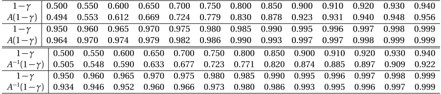
from 1855 . . . 5 Table 2.1 Comparison of (i) the limiting coverageA(1₋γ)versus the credibilty

(1₋γ)(ii) the required credibiltytA−1₍₁₋_γ₎_{versus the target coverage} (1−γ)of a one-sided credible interval. . . 29 Table 2.2 Comparison of obtained coverage and average length of Bayesian

cred-ible intervals forf(x0), with that obtained from a confidence interval. 38 Table 2.3 Proportion of times the test is rejected:f1and f2. . . 38

Table 2.4 Proportion of times the test is rejected:f3and f4. . . 39

Table 2.5 Proportion of times the test is rejected:f5and f6. . . 40 Table 3.1 Comparison of obtained coverage and average length of Bayesian

cred-ible intervals forg(x0), with that obtained from a confidence interval. 65 Table 4.1 Comparison of obtained coverage and average length of Bayesian

credible intervals for f−1₍_y₀₎_{, with that obtained from a confidence}

(10)

LIST OF FIGURES

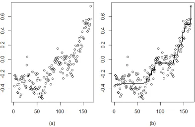
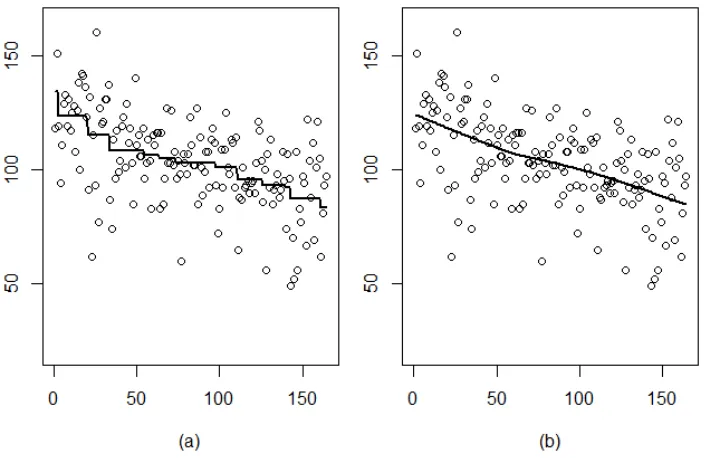
Figure 1.1 (a) Plot of mean annual temperatures with time, based on the global warming data. (b) The plot in (a) with the isotonic regression estimator. 4 Figure 1.2 Scatterplot and the isotonic regression estimate for the warming

trend of Lake Mendota. (a) Raw estimate. (b) A smoothed version of the raw estimate. . . 6 Figure 1.3 Plot of the Canadian income data with the convex regression estimate. 7 Figure 2.1 Plot demonstrating thatΠ(n1/3₍_f∗₍_x₀₎₋_fˆ

n(x0))≤0

D_n)does not have a limit in probability, using three instances of the data. . . 26 Figure 2.2 Obtained coverageA(1₋γ)versus the chosen credibilty(1₋γ). The

dotted line denotesx=y. . . 28 Figure 2.3 Required credibiltyA−1₍₁₋_γ₎_{versus target coverage}₍₁₋_γ₎_{. The dotted}

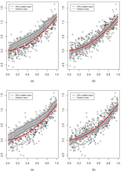
line denotesx=y. . . 28 Figure 2.4 (a) Samples from a truncated normal posterior. (b) Samples from a

projection-posterior. The red line denotes the true function.f0=h1. 33

Figure 2.5 (a) Samples from a truncated normal posterior. (b) Samples from a projection-posterior. The red line denotes the true function.f0=h2. 34

Figure 2.6 (a) Samples from a truncated normal posterior. (b) Samples from a projection-posterior. The red line denotes the true function.f0=h3. 35 Figure 2.7 Global Warming dataset: 95% credible regions. (a) Credible region

from a truncated normal posterior. (b) Credible region from a projection-posterior. . . 36 Figure 2.8 Plots of the functions used for testing monotonicity. . . 39 Figure 4.1 Comparison of the mean absolute errors based on the Bayesian

one-stage and two-one-stage procedures forn=50, 100, 150, 200. . . 90 Figure 4.2 Comparison of the mean absolute errors based on the Bayesian

one-stage and two-one-stage procedures forn=250, 400, 600, 800. . . 91 Figure 4.3 Comparison of the mean absolute errors based on the Bayesian

(11)

CHAPTER

1 INTRODUCTION

(12)

chapters. We start with describing some real life examples involving shape constraints.

1.1 Some motivating examples

1.1.1 Global warming

The global warming dataset provide by Jones et al. (2016) contains the mean annual temper-ature anomalies in Celsius, from 1850 to 2010. Tempertemper-ature anomaly denotes the departure from a long-term average. For this dataset, the long-term average is the mean of the tem-peratures from 1961 to 1990. The data were collected from different meteorological stations both on the land and the sea and corrected for non-climatic errors. The data are tabulated in Table 1.1. Figure 1.1 provides a scatterplot of the temperatures with respect to the years, along with a nonparametric constrained estimator of the underlying function. The plot depicts an increasing trend of temperature with time.

Under the assumption that the function relating the mean annual temperatures to time is monotone increasing, estimation of the function calls for the known problem of iso-tonic regression. The isoiso-tonic regression provides an estimate of the underlying regression function by minimizing the error sum of squares under the monotonicity constraint.

1.1.2 Warming-up of Lake Mendota

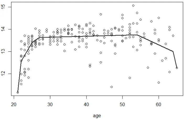
The historical data considered by Barlow and Brunk (1972) on the number of winter days Lake Mendota in Wisconsin freezes per year, shows a decreasing trend over time. The data have been obtained from the R package "isotone". Similar to the data on annual tempera-tures, the nonparamteric estimator in this case is also given by the isotonic regression of the number of freezing days on time. The constraint on the regression function is that of monotone decreasing. Table 1.2 gives the data, and Figure 1.2 gives its scatterplot along with the isotonic estimator and a smoothed version of the estimator.

(13)

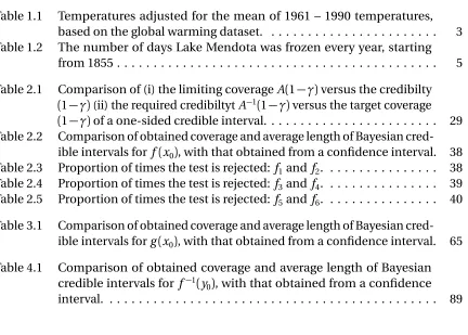
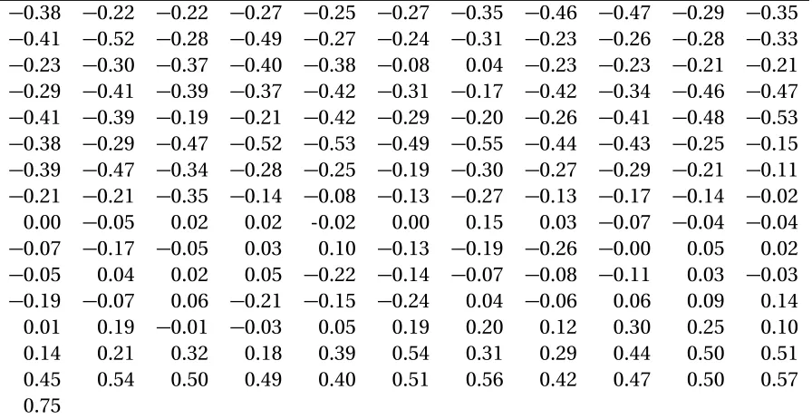
Table 1.1: Temperatures adjusted for the mean of 1961 – 1990 temperatures, based on the global warming dataset.

−0.38 ₋0.22 ₋0.22 ₋0.27 ₋0.25 ₋0.27 ₋0.35 ₋0.46 ₋0.47 ₋0.29 ₋0.35

−0.41 −0.52 −0.28 −0.49 −0.27 −0.24 −0.31 −0.23 −0.26 −0.28 −0.33

−0.23 ₋0.30 ₋0.37 ₋0.40 ₋0.38 ₋0.08 0.04 ₋0.23 ₋0.23 ₋0.21 ₋0.21

−0.29 ₋0.41 ₋0.39 ₋0.37 ₋0.42 ₋0.31 ₋0.17 ₋0.42 ₋0.34 ₋0.46 ₋0.47

−0.41 −0.39 −0.19 −0.21 −0.42 −0.29 −0.20 −0.26 −0.41 −0.48 −0.53

−0.38 ₋0.29 ₋0.47 ₋0.52 ₋0.53 ₋0.49 ₋0.55 ₋0.44 ₋0.43 ₋0.25 ₋0.15

−0.39 ₋0.47 ₋0.34 ₋0.28 ₋0.25 ₋0.19 ₋0.30 ₋0.27 ₋0.29 ₋0.21 ₋0.11

−0.21 −0.21 −0.35 −0.14 −0.08 −0.13 −0.27 −0.13 −0.17 −0.14 −0.02

0.00 ₋0.05 0.02 0.02 -0.02 0.00 0.15 0.03 ₋0.07 ₋0.04 ₋0.04

−0.07 ₋0.17 ₋0.05 0.03 0.10 ₋0.13 ₋0.19 ₋0.26 ₋0.00 0.05 0.02

−0.05 0.04 0.02 0.05 −0.22 −0.14 −0.07 −0.08 −0.11 0.03 −0.03

−0.19 ₋0.07 0.06 ₋0.21 ₋0.15 ₋0.24 0.04 ₋0.06 0.06 0.09 0.14

0.01 0.19 ₋0.01 ₋0.03 0.05 0.19 0.20 0.12 0.30 0.25 0.10 0.14 0.21 0.32 0.18 0.39 0.54 0.31 0.29 0.44 0.50 0.51 0.45 0.54 0.50 0.49 0.40 0.51 0.56 0.42 0.47 0.50 0.57 0.75

The order is in increasing years from left to right and (next) row-wise.

1.2 Shape-restricted estimation

Nonparametric estimation of the underlying function in a major portion of shape-restricted statistical models are based on the concepts of the greatest convex minorant (GCM) and the least concave majorant (LCM) of a cumulative sum diagram of a certain set of points corresponding to the context of the problem. For instance, in monotone regression, the constrained estimator of the regression function, obtained by minimizing the error sum of squares subject to the monotonicity constraint, is the slope (left derivative) of the GCM of

¨

(0, 0),(1/n,Y1/n),(2/n,(Y1+Y2)/n), . . . ,

1,

n

X

i=1 Yi/n

« .

(14)

Figure 1.1: (a) Plot of mean annual temperatures with time, based on the global warming data. (b) The plot in (a) with the isotonic regression estimator.

1.2.1 Asymptotic properties of the constrained estimators

Durot (2002) established that when the true regression functionf0is monotone increasing

and differentiable, the isotonic regression estimator ˆf converges tof0at the raten−1/3under

theL1-metric. In other words,

Z 1

0

|fˆ(t)−f0(t)|dt =O(n−1/3).

Forx0∈(0, 1)such thatf0(x0)exists andf 0(x0)>0, Brunk (1970) established that ˆf(x0)is a

consistent estimator off(x0)and

(_fˆ₍_x₀₎₋_f₀₍_x_{0)) =}_O

P(n−1/3).

Forx0an interior point of[0, 1]with f₀0(x0)>0, Brunk (1970) established the asymptotic

distribution of the constrained point estimator ˆf(x0). ForW1a two-sided standard Brownian

motion on_RandZ1=arg min{W1(t) +t2:t ∈R}, andC =2b(a/b)2/3witha =

Æ σ2

(15)

Table 1.2: The number of days Lake Mendota was frozen every year, starting from 1855 118 151 119 94 111 129 133 119 131 117 125 128 108 126 138 100 142 141 136 123 91 132 62 115 93 160 77 127 120 121 131 131 137 87 74 113 96 117 99 104 119 123 101 129 112 118 103 85 140 111 115 106 106 118 96 103 113 104 83 115 111 116 116 83 116 85 96 127 103 103 126 102 108 96 104 98 60 107 103 98 107 123 111 102 102 127 85 114 101 89 99 108 108 92 113 118 112 93 72 83 109 92 109 125 101

98 113 112 92 114 65 88 87 101 92 93 95 90 94 95

90 103 121 117 104 86 100 56 107 92 113 85 91 93 98

88 91 108 95 74 107 96 49 70 52 108 56 83 77 97

94 67 122 104 88 112 69 101 121 105 62 81 93 97

The order is in increasing years from left to right and (next) row-wise.

andb =f₀0(x0)/2, the asymptotic distribution of ˆf(x0)is given by

n1/3(fˆ(x0)−f0(x0)) C Z1.

A similar result was established in the context for decreasing densities by Prakasa Rao (1969). The distribution ofZ1is known as the standard Chernoff distribution. It is symmetric about zero, with tails tending to zero faster than the standard normal distribution. Its quantiles have been tabulated in Groeneboom and Wellner (2001).

1.2.2 Shape-restricted estimation as a ‘projection’

The shape-restricted estimator of the parameter of interest in all such cases as described above is obtained by minimizing a certain ‘loss function’ under the constraint of shape on the parameter. In regression, for instance, the loss function is the error sum of squares, while for monotone density estimation, the loss function is the negative log-likelihood. The PAVA provides an algorithm for constrained estimation under a wide range of convex loss functions; see Section 3.1 of De Leeuw et al. (2009). The constrained estimator of a function

(16)

Figure 1.2: Scatterplot and the isotonic regression estimate for the warming trend of Lake Mendota. (a) Raw estimate. (b) A smoothed version of the raw estimate.

1.3 Some background on Bayesian nonparametrics

The application of Bayesian principles on nonparametric estimation and inference prob-lems has gained huge popularity in recent times. Bayesian nonparametrics consists of two main steps: specifying a prior distribution on the infinite-dimensional parameter space, and combining the prior with the likelihood using the Bayes formula to obtain the posterior distribution. The development of Markov Chain Monte Carlo (MCMC) sampling method-ologies has popularized the use of Bayesian nonparametrics by providing fast and efficient ways of sampling from the posterior distribution. This subject has enormous applications in engineering, machine learning, genetics, climate science, neuroscience and many more.

(17)

Figure 1.3: Plot of the Canadian income data with the convex regression estimate.

them as compared with the data. The most common methods of prior construction in nonparametric models are

1. finite random series with priors on the coefficients, 2. mixture models,

3. Gaussian processes.

(18)

1.3.1 Posterior consistency and contraction rates

Posterior consistency is the characteristic of the posterior distribution concentrating near the point mass of the true parameter value when the sample size grows large. In finite dimensional parametric models, posterior consistency holds under mild assumptions, but in nonparametric models, more involved conditions are required to be satisfied for posterior consistency to hold. Schwartz (1965) introduced the concept of Kullback-Leibler neighborhoods and exponentially consistent tests to prove posterior consistency in domi-nated statistical models. Ghosal et al. (1999) and Barron et al. (1999) provided extensions of Schwartz’s results.

LetΘbe a parameter space equipped with the Borel-sigma field_B. LetX = (X1, . . . ,Xn)T

denote the observed data. Letd be a metric defined onΘ. LetP_θ(n)denote the joint distri-bution ofX indexed byθ. LetX ∼P_θ(n) and letθ0∈Θbe the true value of the parameter.

LetP_θ0(n)denote the corresponding true joint distribution. LetΠ(·|X)denote the posterior corresponding to the priorΠon the Borel sets ofΘ. The posterior distributionΠ(·|X)is said to be consistent atθ0if for everyε >0,

Π(θ :d(θ,θ0)> ε|X)→Pθ(n0)0, (1.1) asn→ ∞. Posterior consistency tells us that as the sample size grows large, the posterior distribution converges to the point mass atθ0. It also tells us that the posterior distributions

obtained using different priors will agree in the sense that their distances in the weak topology will tend to zero, with sample size going to infinity.

The rate at which the posterior distribution converges to the point mass ofθ₀is formal-ized in what is known as the contraction rate. A sequenceε_n of real numbers withε_n_→0 is a contraction rate atθ₀with respect to the metricd if

Π(θ :d(θ,θ0)>Mnεn

X)→

P_θ(n)

0 0, (1.2)

for everyMn → ∞. A natural problem is then to obtain the fastest possible rate, i.e. the

(19)

where an analytic representation is not available, more elaborate steps are needed. The general theory of posterior contraction developed by Ghosal et al. (2000a) gives a set of conditions on the parameter space and the prior distribution, under which (1.2) holds true. The foremost condition is the existence of test functionsφ_n with exponentially small error for testing

H0:P =P( n)

θ0 , H1:P =P( n)

θ for someθ :d(θ,θ1)> ε,

for someε >0,θ₁ _∈ ΘandX ∼P for some joint distributionP. The null hypothesis is rejected whenφn =1. Such tests are usually constructed by first considering a series of

hypothesis tests where the alternative is a neighborhood separated from the null parameter, and then combining these tests to obtainφn. Combining the tests over the parameter

values whenΘis non-compact is more complicated since the number of balls covering the alternative parameter space may be infinite. For this reason, a condition on the size of an appropriate sieveΘ_n_⊂Θis imposed so that the tests can be combined over the parameter values belonging to the sieve, giving the desiredφ_n. This condition controlling the size of

Θnis given by a condition on the entropy (logarithm of the number of small balls required

to coverΘn) of the sieve. Another key condition requires that the prior gives sufficient mass

to Kullback-Leibler neighborhoods of the true parameterθ0. Finally, the prior mass of the

complement of the sieveΘn needs to be small, so thatΘcan be substituted byΘn in the

testing and entropy conditions. An elaborate theory with technical details on the conditions, depending on the dependence structure ofX has been provided in Ghosal and van der Vaart (2017).

1.3.2 Credible sets and coverage

For a parameter spaceΘ,θ₀_∈Θthe true parameter value andγ_∈[0, 1], a subsetC(X)ofΘ is a 1₋γcredible set if the posterior mass ofC(X)is 1₋γ. In other words,

Π(θ :θ _∈C(X)|X) =1₋γ. (1.3)

(20)

n→ ∞,

P_θ0(n)(θ0∈C(X))→1−γ, (1.4)

in view of the Bernstein-von Mises theorem. Thus in finite-dimensional models, the fre-quentist and Bayesian methods of uncertainty quantification nearly agree for large sample sizes. The credible intervals therefore asymptotically behave as confidence intervals and give the right coverage. In infinite-dimensional parameter spaces, however, the Bernstein-von Mises theorem may not hold, and it has been shown in various instances that credible sets fail to yield the right asymptotic coverage. Under the Gaussian white noise model, Cox (1993) showed that the asymptotic coverage of Bayesian credible sets at any level may be arbitrarily low. The problem of inadequate coverage was further emphasized by Freed-man (1999). It may be noted that both Cox and FreedFreed-man drew the true function from the prior itself, and formulated their conclusions by showing the inadequate coverage in the almost sure sense with respect to the prior. The work of Knapik et al. (2011) provided a more detailed picture of this problem by covering inverse problems. They showed that asymptotically zero coverage occurs by an oversmoothing prior over the truth, while by an undersmoothing prior, conservative credible sets can be obtained with the asymptotic coverages equal to 1. This technique was used in the problem of estimating the initial condition of the heat equation in Knapik et al. (2013).

Leahu (2011) and Castillo and Nickl (2013) showed that if the parameter space is ex-tended beyond the`₂-space of sequences, then the credible sets can yield adequate frequen-tist coverage. Castillo and Nickl (2013) further established parametric posterior convergence rates under negative Sobolev norms, which are weaker than the original`2-norms. They

(21)

1.4 Bayesian nonparametrics in shape-restricted problems

In spite of the spectacular development of Bayesian theory and methods for function es-timation under smoothness regimes, shape-constrained analysis has received much less attention. Bayesian methods are however well suited for shape-restricted problems as the additional qualitative information on shape can be naturally incorporated in the prior. In some situations where the shape constraint on the function leads to a particular represen-tation of the function, Bayesian methods have been used by exploiting that represenrepresen-tation, resulting in a posterior distribution complying with the shape restriction because of that representation. For instance, Williamson (1956) showed that a monotone non-increasing density on[0,∞)can be represented as

g(x) =

Z ∞

0

1[0,z](z)z−1d P(z), (1.5)

whereP is a probability distribution on[0,∞)known as the mixture distribution. Using this mixture representation, Salomond (2014) established nearly minimax contraction rates for a decreasing density by using a Dirichlet mixture of uniform distributions as a prior ong. Further, in the same context, Martin (2017) obtained nearly minimax contraction rates using an empirical prior. Contraction rates have been obtained in a few other occasions such as the current status censoring model with a Dirichlet process prior as an illustration of the general theory in Ghosal et al. (2000a) and Salomond (2018) within testing for monotonicity of a regression function. A more general Bayesian framework for analyzing contraction rates in different shape-restricted problems is therefore lacking. Also, point-wise posterior contraction rates and asymptotic representation of the posterior distribution of the function at a specific point, like the Bernstein-von Mises theorem in parametric models have not been addressed in the literature. In this dissertation, we shall focus on some of the fundamental problems encountered while using nonparametric Bayesian methods in shape-restricted problems.

1.5 Introducing the ‘projection-posterior’

(22)

prior onΘ∗. Because of the structure ofΘ∗, however, the resulting posterior distribution may have a complicated form that may be quite difficult to analyze for frequentist properties. As an alternative approach, consider a prior onΘ, not necessarily concentrated onΘ. The flexibility of a conjugate prior onΘwould result in a posterior distribution easier to analyze and sample from. However, this posterior may not be concentrated onΘ∗_{where the true} parameter is known to lie. To rectify this issue, let us define the ‘projection’ ofθ _∈Θwith respect to the distanced as the element inΘ∗_{closest to}_θ _{in terms of}_d_{. Formally stated,} forθ _∈Θ, the projectionθ∗_{is defined as}

θ∗₌_{arg min} η∈Θ∗

d(θ,η). (1.6)

Note that ifθ _∈Θ∗_{, then by (1.6),}_θ∗₌_θ_{. Under the mapping}_θ _7→_θ∗_{, the induced} distribu-tion of the posterior ofθ is what we would denote by the ‘projection-posterior’. In other words, letΠbe a prior distribution onΘ, and letΠ(·|X)denote the posterior distribution. Withθ∗_{as defined in (1.6), define the projection-posterior}_Π∗_on_Θ∗_as

Π∗

n(θ ∈B) =Π(θ :θ

∗

∈B|X), (1.7)

for every measurableB⊂Θ∗_{. As an example, consider the differential equation model by} Bhaumik and Ghosal (2015). We have a regression modelY = f_θ(t) +",θ _∈Θ_⊂Rp. The function f is assumed to satisfy a constraint given by the system of ordinary differential equations

df_θ(t)

dt =F(t,fθ(t),θ), t ∈[0, 1]. (1.8)

(23)

equations.

Lin and Dunson (2014) proposed a method of Bayesian monotone curve and surface estimation using Gaussian process projections. Samples from the Gaussian posterior were projected on the smooth monotone class of functions. They established posterior consis-tency and obtained contraction rates in terms of the smoothness of the true function. A similar technique was used by Neelon and Dunson (2004).

1.6 Contraction rates under shape constraints

A natural Bayesian approach to a problem where the underlying function has some shape restriction, is to use a prior on the function complying with the shape constraint, and obtain the corresponding posterior satisfying the shape restriction. The main problem with this approach is, however, that the resulting posterior has a complicated form which makes it very challenging to analyze the distribution for contraction rates. On the other hand, an unrestricted prior will result in a conjugate posterior that may not be supported on the shape-restricted class of functions, yielding a posterior not complying with the shape constraint. A possible way to rectify this problem, the one which we will explore in this dissertation, is using an unrestricted prior on the function space, and analyzing a ‘projection-posterior’ introduced in the previous section for consistency and contraction rates, instead of the unrestricted posterior. The distance used to introduce the projection-posterior in our context could be the global or empiricalLp-metrics on function spaces, with 1≤p<∞.

In this case, the projection of a step function generated from the unrestricted posterior can be computed using algorithms similar to the PAVA (see Section 3.1 of De Leeuw et al. (2009)). Letθ∗_{denote the projection of}_θ _{with respect to a distance}_d_{. Then by the property} of projection and the triangle inequality, we have that

d(θ∗,θ0)_≤d(θ∗,θ) +d(θ,θ0)_≤d(θ0,θ) +d(θ,θ0) =2d(θ,θ0), (1.9)

whereθ₀is the true function lying in the constrained parameter space. Using (1.9), we write (1.2) as

Π(θ :d(θ∗,θ0)>Mnεn|X) ≤ Π(θ :d(θ,θ0)>Mnεn/2|X). (1.10)

(24)

inherits the rate of the unrestricted posterior. The unrestricted posterior, in most cases, is easier to analyse for rates, because of the simpler structure resulting from conjugacy.

1.7 Uncertainty quantification in point-wise estimation

un-der shape constraints

With the concept of projection-posterior as a tool for Bayesian estimation of a shape-constrained function, it seems worth exploring if a point estimator resulting from the induced posterior can be used in quantifying uncertainty in estimating the value of the function at a fixed point. Credible sets from the projection-posterior are easy to obtain from posterior sampling and projection using the PAVA, and do not need any bootstrapping or asymptotic distribution. In this dissertation, we obtain a credible set for the value of the shape-restricted function at a fixed point using the projection-posterior in the context of monotone regression and density function. Using concepts from the empirical processes theory, and results on the greatest convex minorant, we establish that the asymptotic coverage of our credible interval has a quantifiable form, and that a re-calibration method will give us a credible interval with the right asymptotic coverage.

Two very interesting implications seem to result from our study. First, we observe that the coverage may be higher than the nominal credibility level, the opposite of the phenomenon observed by Cox (1993) in the context of smooth nonparametric signal estimation. The second, more crucial finding is that both the method of constructing the credible interval and its asymptotic coverage do not involve the constants involving the true function. This is in contrast with the uncertainty quantification using confidence intervals in the frequentist approach, where calculating the margin of error requires estimating the derivative of the function at the fixed point. Our construction of the credible interval thus eliminates the uncertainties resulting from estimating any nuisance parameters.

1.8 Bayesian testing for monotonicity

A traditional Bayesian approach for testing the hypothesisH0:θ ∈ F versusH1:θ /∈ F,

whereF is a class of shape-restricted functions, would be employing the Bayes factor and rejectingH0wheneverθ falls outsideF. This approach, however, has a major limitation as

(25)

parts. Salomond proposed the idea of ‘enlarging’ the null hypothesis by a multiple of the contraction rate corresponding toθ ∈ F. In other words, he showed that for an appropriate τnand a distanced, testing for

H0:d(θ,F)≤τn versus H1:d(θ,F)> τn

leads to consistency underH0and high power againstα-smooth alternatives with an opti-mal separation rate. Adapting Salomond’s idea, we propose a Bayes test for monotonicity of a regression or density function by employing the distance of f from its projection f∗ on the constrained space. Our test is shown to be computationally simpler than the test proposed by Salomond and universally consistent. For any fixed f0∈ F, the Type I error

goes to zero, and for any fixed f0∈ F/ , the Type II error goes to zero. Also, our test has high

power against smooth alternatives sufficiently separated from_F0.

1.9 Bayesian two-stage monotone regression quantile

esti-mation

Estimating a regression quantile of a monotone increasing regression function can be viewed as an inverse regression problem. In this dissertation, we use the projection-posterior for a regression function to estimate a monotone increasing function. We obtain a cred-ible set for a regression quantile that has the appropriate asymptotic coverage. We then obtain a sampling interval from the posterior of the regression quantile and generate the second-stage observations with the predictors belonging to that sample. By representing the regression function on this interval as a linear function, we use a Gaussian prior on the coefficients and analyze the second-stage posterior distribution of the regression quantile and find that the second stage estimator obtains the parametricn−1/2_{-rate of contraction.}

1.10 Notations

In this section, we describe the notations and assumptions used in this dissertation. For two sequences of real numbersanandbn,an®bn oran=O(bn)means thatan/bn is bounded,

(26)

We sayZ ∼NJ(µ,Σ)ifZ has a J-dimensional normal distribution with meanµand

covariance matrixΣ. Let the space of real-valued monotone increasing functions on[0, 1] be denoted by_F, and the space of monotone increasing functions on[0, 1]bounded in absolute value byK >0 be denoted by_F(K). A real-valued functionf on[0, 1]is calledα -Hölder continuous for someα_∈(0, 1)if there exists someL>0 such that for allx,y ∈[0, 1],

|f(x)−f (y)| ≤ |x−y|α. The set ofα-Hölder continuous functions on[0, 1]is denoted by

H(α,L). ForT ⊂R,L∞(T)denotes the set of all uniformly bounded real functions onT. For 1_≤p <∞andx ∈Rk, letkxkp = (Pk_l₌₁|xl|p)1/p andkxk∞=max1≤l≤k|xl|. ForG

a probability measure on[0, 1]and f :[0, 1]_7→RsatisfyingR₀1|f|pd G <∞, letkfkp,G =

(R1

0 |f |

p_{d G}₎1/p_{. The indicator function of a set}_U _{is denoted by}₁ U(·).

Let E0(·)and Var0(·)be the expectation and variance operators taken under the true dis-tributionP0. We writeY = (Y1, . . . ,Yn),X = (X1, . . . ,Xn),Dn= (Y,X),F0= (f0(X1), . . . ,f0(Xn))

and"= ("₁, . . . ,"_n). Let_P_n denote the expectation with respect to the empirical measure. Let

p_f(n_,_σ)(Y|X)be the conditional probability density ofY givenX under the working assump-tion of normality of errors with varianceσ2_{in (2.0.1). For an}_m_×_m _matrix_A

1, letλmin(A1)

andλmax(A1)be the smallest and largest eigenvalues respectively. For anotherm×mmatrix A2, the relationA1≤A2means thatA2−A1is non-negative definite. LetIm stand for the m×m identity matrix.

For a random variableY and a sequence of random variablesXn,Xn Y means that

Xn converges in distribution toY,Xn→P Y means thatXnconverges toY inP-probability.

For random variablesX andY,X =d Y means thatX andY have the same distribution. Theε-covering number of a setAwith respect to a metricd, denoted by_N(ε,A,d), is the minimum number of balls of radiusεneeded to coverA.

For f :[0, 1]_7→_Randd a distance metric on real valued functions, let the projection of

f on_F with respect to a distanced be the function f∗_{that minimizes}_d₍_f_,_h₎_over_h_{∈ F}_. Also, letd(f,_F)denoted(f,f ∗₎_{. Let}_Π∗_{denote the induced posterior distribution of}_f∗_.

1.11 Chapter organization

(27)

piece-wise constant functions havingJ knots is of the orderJ−1_{and this rate can be achieved}

when the knots are equidistant on[0, 1]. Forp>1 however, equidistant knots may only give the approximation rate J−1/p_{, but the rate}_J−1_{of approximation can be restored by varying}

the locations of the knots. For the Bayesian method, this will therefore need assigning a prior on the location of the knots, in addition to the prior on the coefficients of the step function. We develop contraction rates under both these settings and achieve the minimax raten−1/3_for_p₌_{1 and up to a logarithmic factor for}_p _>_{1, under the empirical}_Lp_-distance.

For a point-wise confidence interval, we derive the asymptotic distribution of the sieve-maximum likelihood estimator under monotonicity. The asymptotic distribution of the point-wise projection-posterior is then developed, and a credible interval is obtained, whose asymptotic coverage can be analytically characterized. We then use a re-calibration method to obtain a credible interval with the right asymptotic coverage. Similar procedures are performed for monotone density estimation as well. In summary, we demonstrate the properties of Bayesian nonparametric methods through the following examples of shape-restricted problems.

1.11.1 Rates, coverage and tests in Bayesian monotone regression

Using a finite random step function prior on the regression functionf with equispaced knots on[0, 1]and Gaussian priors on the coefficients, we analyze the projection-posterior to obtain contraction rates in terms of the global and empiricalL1-distances. Using a finite

random step function prior on f with an additional prior on the location of the knots, we obtain nearly minimax contraction rates in terms of the empirical Lp-distance. We

construct a point-wise projection-posterior credible interval and show that it gives the right asymptotic coverage. We finally develop a universally consistent Bayes test for monotonicity and show that it has optimal power properties. The asymptotic distribution of a constrained sieve-maximum likelihood estimator has been established.

1.11.2 Rates, coverage and tests in Bayesian monotone density

estima-tion

In the setup of a monotone non-increasing density on the positive real line, we use a finite random histogram prior on the density functiong with a Dirichlet prior on the coefficients and analyze the projection-posterior for contraction rates in terms of theL1

(28)

credible interval and show that it gives the right asymptotic coverage. We finally develop a universally consistent Bayes test for monotonicity of the density and show that it has optimal power properties. The asymptotic distribution of a constrained sieve-maximum likelihood estimator is also established.

1.11.3 Bayesian two-stage regression quantile estimation with

acceler-ated contraction rate

Using concepts from the projection-posterior credible set for the point-wise regression estimator, we establish an−1/3_{contraction rate for and obtain a credible set that has the}

right asymptotic coverage. We then construct a sampling interval from the first-stage posterior and show that its credibility and coverage tend to 1 asymptotically. Using this sampling interval, we sample the second stage observations with the predictors from this interval. Representing f as a linear function on the interval, we use a Gaussian prior on the coefficients to obtain a posterior distribution of the regression quantile using the second-stage data. We show that the second-second-stage posterior achieves the parametricn−1/2_{-rate of}

(29)

CHAPTER

2 RATES, COVERAGE AND TESTS FOR

BAYESIAN MONOTONE REGRESSION

Consider the nonparametric regression model for a response variableY with respect to a predictor variableX ∈[0, 1]given by

Y =f(X) +", (2.0.1)

where f is a monotone increasing function on[0, 1]and"is a mean-zero random error with finite varianceσ2. Let us observen replications(Y1,X1), . . . ,(Yn,Xn), where the design

pointsX1, . . . ,Xnare either deterministic or are assumed to have been randomly sampled

from a distributionG having a densityg which is positive on[0, 1]. The error is assumed to be distributed independently of the predictors.

(30)

and De Leeuw et al. (2009)). The constrained point estimator was shown to converge at a raten−1/3_{, and its asymptotic distribution was evaluated by Brunk (1970). Durot (2002)}

studied the global convergence rates of the constrained maximum likelihood estimator of

f and established that when the true regression functionf0is monotone increasing and

differentiable, the isotonic regression estimator ˆf converges to f0at the raten−1/3under

theL1-metric.

A Bayesian approach to such problems would involve approximatingf with a random series function, putting a prior on the coefficients and analyzing the behavior of the poste-rior distribution for contraction rates and uncertainty quantification. Posteposte-rior contraction rates in the nonparametric regression setup have been well studied in the literature, but Bayeisan inference under the monotonicity constraint has received relatively less attention. Shively et al. (2009) followed a Bayesian approach by using a mixture of constrained normal distributions as a prior for the spline coefficients. Bayesian nonparametric methods have been developed for other shape-constrained problems, such as monotone density and current status. Salomond (2014) established the nearly minimax raten−1/3_{for a decreasing}

density using a prior of a mixture of uniform densities.

Testing for monotonicity of a regression function has been studied following various approaches both in frequentist and Bayesian literature; see Akakpo et al. (2014), Hall and Heckman (2000), Baraud et al. (2005), Ghosal et al. (2000b) and Bowman et al. (1998). Salomond (2018) showed that when a monotone f is near the boundary, the traditional Bayes factor approach would often fail to identify it correctly, a problem that can be rectified by enlarging the null hypothesis so that monotone functions near the boundary are correctly classified with high posterior probability.

The rest of the chapter is organized as follows. Section 2.1 states some assumptions and describes the priors. Results on the contraction rates of f and those on the point-wise credible intervals are presented in Sections 2.2 and 2.3 respectively. The Bayesian test for monotonicity is developed in Section 2.4. Simulation results related to point-wise credible intervals and the testing procedures are discussed in Section 3.4. Proofs of the results are provided in Section 2.6 and Section 2.7.

2.1 Assumptions and Priors

For Xi ∈ [0, 1],i = 1, . . . ,n, and I1, . . . ,IJ a partition of [0, 1] into J disjoint intervals, let

(31)

empirical distribution of the design points. LetG be a measure on[0, 1]with continuous and positive densityg satisfying

a1<g <a2,

for some 0<a1<a2<∞. If the design points are fixed, we assume thatGnsatisfies

sup

x∈[0,1]

G_n([0,x])−G([0,x])

=o(n−1/3). (2.1.1)

For randomX, we assume that

Xi i.i.d.

∼ G. (2.1.2)

With a slight abuse of notation, we shall useGn andG to denote the corresponding distri-bution functions as well. We have the following the assumption on the true distridistri-bution

P0.

Assumption A. Under the true distribution P0, Yi = f0(Xi) +"i, such that"i are i.i.d. sub-Gaussian with mean0and varianceσ2

0for i =1, . . . ,n .

We construct priors on f by representingf as a piece-wise constant function on[0, 1] with J the number of pieces. The knots of f may be equally-spaced on[0, 1]or may be chosen randomly from the design pointsX1, . . . ,Xn. We represent the model in (2.0.1) as Y =Bθ +". We use the following types of priors on f.

1. Type1: For a deterministic J, letIj = ((j−1)/J,j/J], 1≤ j ≤ J. We represent f as f(·) =PJ

j=1θj1Ij(·), and use the priorθ ∼NJ(ζ,σ

2_Λ)_where_k_ζ_k

∞is bounded, andΛ a J×J diagonal matrix with diagonal entriesλ2

1, . . . ,λ 2

J, withB1< λj <B2for some B1,B2>0.

2. Type 2: Using a deterministic J, letIj = [ξj−1,ξj), 1≤ j ≤ J, withξ0=0. We write f(·) =PJ_j₌₁θj1Ij(·), withξ= (ξ1, . . . ,ξJ)andθ having the joint prior

π(ξ) =

n J −1

−1

1

ξj ∈X,ξj < ξj+1, 1≤j ≤J −1, ξJ =1

, θ ∼N_J(ζ,σ2Λ).

(32)

For the Prior 1, the error varianceσ2_{may be estimated by maximizing the marginal}

likeli-hood ofσor by endowingσ2with an inverse-gamma prior with parameters(β1/2,β2/2),

whereβ₁>4,β₂>0. Observe thatY|σ∼N_n Bζ,σ2₍_B_Λ_BT₊_I_n)

. Maximizing the corre-sponding marginal log-likelihood with respect toσ2_{, we obtain}

Ò σ2

n=n

−1₍_Y

−Bζ)T(BΛBT+In)−1(Y −Bζ). (2.1.3)

The plug-in posterior distribution of f is obtained by substituting_Òσn forσ. In Prior 2, for a

pre-fixed large constantS0, we use the uniform distribution on(0,S0)as a prior forσ.

2.2 Posterior contraction rates under monotonicity

In order to establish posterior contraction rates forf with unknownσ, we first show that the maximum marginal likelihood estimator forσ2_{in the plug-in Bayes approach or the}

marginal posterior distribution ofσ2_{in the fully Bayes approach, are consistent uniformly}

forf0∈ F(K).

Proposition 2.2.1. For f0∈ F(K), and the prior on f of Type1, if J → ∞and J n , then under Assumption A on the errors,

(a) the maximum marginal likelihood estimatorÒσ

2

nconverges in probability toσ 2 0at the ratemax{n−1/2_,_n−1_J_}_.

(b) Ifσ2_∼_IG₍_β

1/2,β2/2)withβ1>4,β2>0, then the marginal posterior distribution of

σ2_{contracts at the rate}_max_{_n−1/2_,_n−1_J_}_.

We impose monotonicity on f by projectingf on_F using the algorithm for isotonic regression. LetΠ∗

nbe the distribution induced by the posterior of f defined as

Π∗

n(f ∈B) =Π(f :f

∗_∈_B_|_D

n),

for everyB measurable with respect toP i. The induced distributionΠ∗_n, or the projection-posterior, is easier to handle theoretically than a posterior distribution obtained by a prior complying with the monotonicity constraint. For a monotone f0 and f∗ denoting the

projection of f onto _F with respect to a distanced, we have d(f∗_,_f₎ _≤_d₍_f

0,f)by the

property of projection. From this, and using the triangle inequality, we have that

(33)

The projection f∗_{corresponding to a distance}_d _{therefore inherits the contraction rate} of f at a monotonef0with respect tod. Forp≥1, theLp-projection of a step function is

computable, by algorithms similar to the PAVA (see Section 3.1 of De Leeuw et al. (2009)).

2.2.1 Contraction rates under the

L

₁

-metric

In the following theorem, we shall derive contraction rates for the projection-posterior when f0is monotone increasing, in terms of theL1-metric.

Theorem 2.2.2. Let f0 ∈ F(K)and let the prior on f be of Type1, with J → ∞and J n . Letσ2 _{be estimated using the plug-in Bayes approach or endowed with the} inverse-gamma prior using a fully Bayes approach. Then under Assumption A on the errors, for

εn=max{J−1,(J/n)1/2}and every Mn→ ∞, the following assertions hold. (a) For fixed design points satisfying(2.1.1),

E₀Π∗_n _kf −f0k1,Gn >Mnεn

→0.

(b) For random design points satisfying(2.1.2),

E₀Π∗_n _kf −f0k1,G >Mnεn

→0.

In particular, when J n1/3_{, the projection-posterior contracts at the minimax rate}

εn=n−1/3in either case.

2.2.2 Contraction rates under the empirical

L

_p

-metric

When the metric under consideration isLp withp >1, the approximating step function

with equal intervals without additional smoothness may have only J−1/p_{approximation}

rate. A prior on the knots is therefore required for obtaining the optimal contraction rate. For the case ofLp-metric, we shall assume that the true error varianceσ2

0is restricted to the

interval(0,S2

0)for some knownS0large enough. We shall consider deterministic predictors,

and derive a posterior contraction rate based on the empiricalLp-metric.

The following result gives a contraction rate for the projection-posterior under the em-piricalLp-distance when the prior onf constitutes of a prior on the knots and independent

(34)

Theorem 2.2.3. Let f0 ∈ F(K)and the prior on f be of Type2, with J n1/3(logn)t1 for some t1>0. Let the prior onσbe the uniform distribution on(0,S0)for a pre-fixed S0. Let

f∗ _{be the projection of f on}_F _{with respect to the empirical L}

p-metric. Then under the

additional assumption that the errors"i, i =1, . . . ,n , are i.i.d. normal with mean zero and known varianceσ2

0, the posterior distribution of f∗contracts at the rateεn=n−1/3(logn)t2, for t2≥(1+t1)/2.

For the empiricalL2-distance, Theorem 2.2.3 also holds true under Assumption A on the error distribution. As the true regression function is correctly specified, the modified neighborhood ˜B(pf∗,εn;f0)in Theorem 8.40 of Ghosal and van der Vaart (2017) reduces

to anL2-ball around f0, and the assumptions of the theorem follow in an exactly similar

manner as derived in the proof of Theorem 2.2.3.

The assumption ofσ₀being restricted to a bounded domain(0,S0)is fairly mild, and allows one to construct the exponentially consistent tests required in the general theory of posterior contraction, using arguments similar to Lemma 8.27 of Ghosal and van der Vaart (2017). Nearly optimal contraction rates may be possible to obtain by relaxing this assumption, if we use the arguments from the proof of Theorem 4.1 of Ning and Ghosal (2018) to construct the tests, with a prior onσhaving sufficiently quickly decreasing tails. It would be interesting to obtain nearly optimal contraction rates for the continuous

Lp-metrics, but we do not know about an appropriate prior that would yield the desired

result. In the situation of continuous metrics, the weak approximation with equal intervals produces only a sub-optimal raten−1/(p+2)_{, while with a prior on the knots, the completely}

arbitrary nature of the knots for arbitrary monotonef0does not allow a good prior

concen-tration needed for the optimal contraction rate.

2.3 Uncertainty quantification in point-wise estimation

Let the data be observed from the modelY =f (X) +", where f is a monotone increasing function from[0, 1]toR, bounded in absolute value by someK >0, and the error"under the working model is Gaussian with mean zero and varianceσ2. Letx0∈(0, 1)be such that

f0

0(x0)exists andf00(x0)>0. The isotonic regression estimator off under the constraint that f is monotone increasing, is obtained by minimizing the sum of squaresPn

i=1(Yi−f(Xi))2

subject tof is non-decreasing on[0, 1]. Without loss of generality, we assume thatX1≤ · · · ≤ Xn. From the algorithm for isotonic regression as described in Section 2.1 of Groeneboom

(35)

of the slope (left-derivative) of the greatest convex minorant of the graph of

(0, 0), ₁ n, Y1 n , ₂ n,

Y1+Y2 n , . . . , 1, Pn

i=1Yi n

,

at the pointx0.

Now let f be a monotone increasing piece-wise constant function on[0, 1]. ForJ >1, let f =PJ_j₌₁qj1Ij, where(q1, . . . ,qJ)∈R

J _with_q

1≤ · · · ≤qJ. Consider a sieveΘJ defined as

ΘJ =

(

f = J

X

j=1

qj1Ij :q1≤ · · · ≤qJ, Ij = _j₋₁

J , j J

, 1≤j ≤J

) .

The sieve-maximum likelihood estimator of f , denoted by ˆfn, under the monotonicity

constraint onf , is obtained by minimizing the error sum of squaresPn

i=1(Yi−fˆn(Xi))2as J

X

j=1

X

i:Xi∈Ij

(Yi−qj)2= J

X

j=1

X

i:Xi∈Ij

(Yi−Yj¯)2+ J

X

j=1

Nj(Yj¯ −qj)2.

As the first term is free ofq, it is sufficient to minimize the second termPJ_j₌₁Nj(Y¯j−qj)2

subject to q1 ≤ · · · ≤ qJ. This is equivalent to minimizing the weighted sum of squares

PJ

j=1(Nj/n)(Yj¯ −qj)

2_{subject to the ordering constraint}_q1_{≤ · · · ≤}_qJ_{. From the algorithm for}

weighted isotonic regression, we get that the optimal value ofqj is the left-derivative of the

greatest convex minorant of the graph of ¨

(0, 0), _N

1 n ,

N1 n Y¯1

, . . . ,

_J X

k=1 Nk

n , J

X

k=1 Nk

n Y¯k

«

, (2.3.1)

at the pointP_kj₌₁Nk/n.

We consider the projection-posterior credible interval for f(x0)for a Type 1 prior. The posterior samples of f need not be monotone, so we impose monotonicity by projecting each sample onto F using the isotonization algorithm, to obtain the projection f ∗ ₌ PJ

j=1θj∗1Ij whereθ ∗

j equals the left-derivative of the greatest convex minorant of the graph

of

¨

(0, 0), _N

1 n ,

N1 n θ1

, . . . ,

_J X

k=1 Nk

n , J

X

k=1 Nk

n θk

«

(36)

at the pointP_kj₌₁Nk/n.

Define the unconditional probability(P0×Πn)as

(P0×Πn) f :f ∈B

=E0 Π(f :f ∈B|Dn)

,

for everyB measurable with respect toΠ. The following result gives the unconditional asymptotic distributions ofn1/3₍_f∗_(x0)₋_f0(x0))_and_n1/3₍_fn(x0)ˆ ₋_f0(x0))_.

Theorem 2.3.1. Let the prior on f be of Type1with n1/3_J _n2/3_{. Let W}

1,W2be indepen-dent two-sided Brownian motions onRwith W1(0) =W2(0) =0, Z2=arg min{W1(t) +W2(t) + t2_:_t _∈

R},Z1=arg min{W1(t) +t2:t ∈R}, and C =2b(a/b) 2/3

with a =Æσ2

0/g(x0)and b =f0

0(x0)/2. LetX be random, satisfying(2.1.2). Then under Assumption A on the errors, the following assertions hold.

(a) For every z∈R,P0(n1/3(fnˆ(x0)−f0(x0))≤z)→P(C Z1≤z).

(b) For every z∈R, P0×Πn

(n1/3₍_f∗_(x0)₋_f0(x0))_≤_z₎_→_P_{(C Z2}_≤_z_).

(c) The conditional process z 7→Π(n1/3₍_f∗₍_x₀₎₋_fˆ

n(x0))≤z

D_n)does not have a limit in

probability.

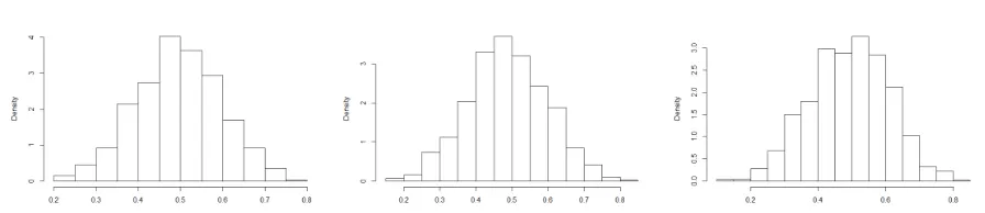
Figure 2.1: Plot demonstrating thatΠ(n1/3₍_f∗₍_x₀₎₋_fˆ_n(_x₀₎₎_≤₀

D_n)does not have a limit in probability, using three instances of the data.

It follows from part (c) of Theorem 2.3.1 that for∆∗

n =n

1/3₍_f∗₍_x₀₎₋_fˆ

n(x0)), and any z ∈R,Π(∆∗n≤z|Dn)cannot converge to a constant (depending onz). This phenomenon

is similar to the problem of the inconsistency of the bootstrap estimator as pointed out by Kosorok (2008) and Sen et al. (2010), in the context of monotone density estimation. We illustrate this by drawing samples of Π(∆∗

(37)

withn =2000 and f0(x) = x2₊_x_/_{5. Figure 2.1 shows that the limit of}_Π₍_∆∗

n ≤0|Dn) is

undoubtedly non-degenerate. It is therefore not possible to construct a credible interval forf(x0)by an approach along the lines of the classical Bernstein-von Mises theorem.

We shall now evaluate the weak limit ofΠ(n1/3₍_f∗₍_x₀₎₋_f₀₍_x₀₎₎_≤_z _|_D

n)and use it to

quantify the limiting coverage of credible sets using projected posterior quantiles. As defined in Theorem 2.3.1, letW1,W2be independent two-sided standard Brownian motions starting

at zero,a =Æσ₀2/g(x0), andb =f 0

0(x0)/2. Define stochastic processesFn∗andF∗onRas F_n∗(z|Dn) =Π n1/3(f∗(x0)−f0(x0))≤z |Dn

,

F_a,b∗ (z|W1) =P

2b(a/b)2/3arg min

t∈R

V(t)≤z |W1

, (2.3.3)

whereV(t) =W1(t) +W2(t) +t2. For everyn≥1,γ∈[0, 1], define

Qn,γ=inf

z ∈R:Π(f∗(x0)≤z|Dn)≥1−γ ,

In,γ= [Qn,1−2γ,Qn,γ2], ∆ ∗

W1,W2=arg min

t∈R

W1(t) +W2(t) +t2 . (2.3.4)

We then have the following result. Theorem 2.3.2. Let F∗

n(·), Fa∗,b(·), Qn,γ, In,γ and∆∗W1,W2 be as defined in(2.3.3)–(4.2.1), with

a =Æσ2₀/g(x0)and b=f₀0(x0)/2. Then forX satisfying(2.1.2)and under Assumption A on the errors,

(a) for every z∈R, Fn∗(z|Dn) Fa,b∗ (z|W1); (b) the distribution of F∗

a,b(0|W1)is symmetric about1/2; (c) the limiting coverage of In,γis characterized as follows:

P₀ f0(x0)∈In,γ

→Pγ

2≤ P(∆ ∗

W1,W2≥0

W1) ≤1− γ 2

=Pγ 2 ≤ F

∗

a,b(0|W1) ≤1−

γ 2

.

For everyu∈[0, 1], define

A(u) =P(P(∆∗_W 1,W2≥0

W1)≤u). (2.3.5)

Also, for everyv ∈[0, 1], defineA−1_(v₎_{as the solution to}_A(u_{) =}_v_{. For a one-sided credible}

(38)

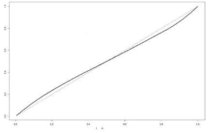
Figure 2.2: Obtained coverageA(1₋γ)versus the chosen credibilty(1₋γ). The dotted line denotesx =y.

Figure 2.3: Required credibiltyA−1₍₁₋_γ₎_{versus target coverage}₍₁₋_γ₎_{. The dotted line}

Bayesian Inference Under Shape Constraints.

ABSTRACT

BIOGRAPHY

ACKNOWLEDGEMENTS

TABLE OF CONTENTS

LIST OF TABLES

LIST OF FIGURES

CHAPTER

1

INTRODUCTION

1.1

Some motivating examples

1.1.1

Global warming

1.1.2

Warming-up of Lake Mendota

1.2

Shape-restricted estimation

1.2.1

Asymptotic properties of the constrained estimators

1.2.2

Shape-restricted estimation as a ‘projection’

1.3

Some background on Bayesian nonparametrics

1.3.1

Posterior consistency and contraction rates

1.3.2

Credible sets and coverage

1.4

Bayesian nonparametrics in shape-restricted problems

1.5

Introducing the ‘projection-posterior’

1.6

Contraction rates under shape constraints

1.7

Uncertainty quantification in point-wise estimation

un-der shape constraints

1.8

Bayesian testing for monotonicity

1.9

Bayesian two-stage monotone regression quantile

esti-mation

1.10

Notations

1.11

Chapter organization

1.11.1

Rates, coverage and tests in Bayesian monotone regression

1.11.2

Rates, coverage and tests in Bayesian monotone density

estima-tion

1.11.3

Bayesian two-stage regression quantile estimation with

acceler-ated contraction rate

CHAPTER

2

RATES, COVERAGE AND TESTS FOR

BAYESIAN MONOTONE REGRESSION

2.1

Assumptions and Priors

2.2

Posterior contraction rates under monotonicity

2.2.1

Contraction rates under the

L

-metric

2.2.2

Contraction rates under the empirical

L

-metric

2.3

Uncertainty quantification in point-wise estimation