A Power Series Based Controller for the Stabilization of a Single Inverted Pendulum on a Cart: Analysis and Real-Time Implementation

(1)

A Power Series Based Controller for the

Stabilization of a Single Inverted Pendulum on a

Cart: Analysis and Real-Time Implementation

Emese Kennedy, and Hien Tran,

Member, SIAM

Abstract—The single inverted pendulum (SIP) system is a classic example of a nonlinear under-actuated system. In the past fifty years many nonlinear methods have been proposed for the swing-up and stabilization of a self-erecting inverted pendulum, however, most of these techniques are too complex and impractical for real-time implementation. In this paper, the successful real-time implementation of a nonlinear controller for the stabilization of a SIP on a cart is discussed. The controller is based on the power series expansion of the solution to the Hamilton Jacobi Bellman (HJB) equation. While the performance of the controller is similar to the traditional linear quadratic regulator (LQR), it has some important advantages. First, the method can stabilize the pendulum for a wider range of initial starting angle. Additionally, it can also be used with state dependent weighting matrices, Q and R, whereas the LQR problem can only handle constant values for these matrices. We present results with both constant and state-dependent weighting matrices. Furthermore, we analyze both the stability region and the disturbance rejection of the controller.

Index Terms—Hamilton-Jacobi-Bellman equation, inverted pendulum, nonlinear feedback control, power series approxima-tion, real-time implementaapproxima-tion, stabilization

I. INTRODUCTION

I

N 1990 the International Federation of Automatic Control (IFAC) Theory Committee published a set of benchmark problems that can be used to compare the benefits of new and existing control methods. One of these problems involves the stabilization of an inverted pendulum [1]. Despite its simple structure, the inverted pendulum is among the most difficult systems to control. This difficulty arises because the equations of motion governing the system are inherently nonlinear and because the upright position is an unstable equilibrium. Furthermore, the system is under-actuated as it has two degrees of freedom, one for the cart’s horizontal motion and one for the pendulum’s angular motion, but only the cart’s position is actuated, while the pendulum’s angular motion is indirectly controlled. Many of the previously proposed nonlinear control techniques for the stabilization of an inverted pendulum are too complex and impractical for real-time implementation [2]. In this paper, we present the successful real-time implementation of a nonlinear controller for the stabilization of a single inverted pendulum (SIP) on a cart. The controller is based on the power series approximation to the solution to the Hamilton

E. Kennedy is with the Department of Mathematics & Statistics, Hollins University, Roanoke, VA 24020; email: [email protected]

H. Tran is with he Department of Mathematics, North Carolina State University, Raleigh, NC 27695 email: [email protected]

Manuscript received 10/13/17.

Jacobi Bellman (HJB) equation [3]–[6]. In addition to our previously presented work [7], [8], we also present results using state-dependent weighting matrices, and analyze both the stability region and the disturbance rejection of the controller.

A. Existing Control Methods

Because of its popularity and numerous applications, there are many existing control methods for the inverted pendulum. However, many of the published controllers have only been tested in simulations and not in real-time experiments. Com-paring experimental results with published work of others, the simulation results are often different from the real-time results. This is because almost all simulations use a simplified model to represent the dynamics of the inverted pendulum. Furthermore, most of the simulations ignore the effects of friction, and often fail to incorporate some physical restrictions like the maximum deliverable voltage by the amplifier, the capacity of the DC motor that drives the cart, and the finite track length.

Below is a summary of the most popular control methods that have been implemented for an inverted pendulum, and a short discussion of the advantages and disadvantages of each method. Most of the cited references were compiled based on an extensive survey by Boubaker [2].

• Fuzzy logic and neural network controllers like the ones presented in [9]–[11] have a simple structure and don’t require lengthy computations. They are very popular methods for both the swing-up and the stabilization of the pendulum, however, the presentation of these methods often lack the specification of the stability conditions. • Proportional-integral-derivative (PID) adaptive control is

discussed in [12]–[14]. This method is good for stabi-lizing the pendulum, but requires frequent tuning. Chang et al. discusses the implementation of a self-tuning PID controller using a Lyapunov approach in [13], but only simulation results are presented without discussion of real-time experiments.

• Energy-based control is one of the most popular and effi-cient methods for swinging-up the pendulum. The global stability conditions of this approach are well proven using Lyapunov techniques. Hybrid control methods based on the energy approach that accomplish both the swing-up and the stabilization of the pendulum without switching controllers are presented in [15]–[19].

(2)

that are not under actuated. In [20] a modified Van der Pol oscillator is implemented for both the swing-up and the stabilization of the pendulum, but with some performance issues. Namely, the fast switching in the implemented controller causes undesirable chattering. In [21] an aggressive sliding mode control law is presented for both the swing-up and the stabilization along with results of numerical simulations for the cart pendulum system, and real-time experimental results for the rotary pendulum system.

• Linear quadratic regulator (LQR) is a simple and easy to implement control method that performs reasonably well for stabilizing the inverted pendulum. However, the performance of the method greatly depends on the selection of the weighting matrices, Q and R, in the cost functional. In a recent publication, Trimpe et al. proposed a self-tuning LQR approach using stochastic optimization, but the method has only been implemented in simulations and not in real-time experiments [22]. • Linear quadratic gaussian (LQG) is a controller that

com-bines LQR with a Kalman Filter to improve disturbance rejection. This method was implemented by Eide et al. in [23] during the balance of an inverted pendulum mobile robot, however, they found that the LQR produced better response when compared to the LQG approach.

• Approximate linearization is a method of finding a non-linear change of coordinates for a nonnon-linear system to construct a linear approximation of the plant dynamics accurate to second or higher order. Starting with the work of Krener [24]–[26], many variants of this approach have been suggested [27], [28]. The algorithm presented in [24] was implemented for the stabilization of a rotary pendulum by Sugie and Fujimoto [29]. They showed through experiments that the method enlarges the stability region. Using the ideas in [25] and [28], Ohsumi and Izumikawa implemented in real-time a control method that can be used for both the swing-up and stabilization of an inverted pendulum on a cart [30]. Based on Krener’s approach, Guzzella and Isodori developed a simpler and more direct method to calculate the quantities involved [31]. This algorithm was implemented for the stabiliza-tion of a cart-pendulum system by Renou and Saydy [32]. Their simulation and experimental results show a slight improvement in the system’s transient response, but a reduced region of stability when compared to the LQR control method. In [33], Ingram et al. present the suc-cessful real-time implementation of a modified approach using an algorithm designed for feedback linearizable systems. Their technique works for both the swing-up and stabilization of an inverted pendulum on a cart. They consider both the finite track length, and the restriction on the maximum voltage input, but they do not take the effects of friction into account.

• State-dependent Riccati equation (SDRE) based con-troller has been used for the stabilization of the pendulum in simulations in [34], [35]. In [36], Dang and Lewis present the successful real-time implementation of a SDRE based controller for both the swing-up and the

0 x

y

Fc >0

M

x

yp

Mp

xp

`p

α

˙ α >0

Fig. 1. Single inverted pendulum diagram.

stabilization. The drawback of this method is that it is computationally very intense as it requires the solution of complicated state-dependent Riccati equations at every time step.

Most of the control methods discussed above ignore the effects of friction. There is a limited number of publications that consider friction in the development of the model for the inverted pendulum. Campbell et al. have studied the use of different friction models during real-time implementation for the stabilization of the pendulum [37], [38]. They have also showed that disregarding friction produces oscillatory behavior during stabilization.

II. SYSTEMDYNAMICS

A. System Representation and Notations

Fig. 1 shows a diagram of the Single Inverted Pendulum (SIP) mounted on a cart. The positive sense of rotation is defined to be counterclockwise, when facing the cart. The perfectly vertical upward pointing position of the inverted pendulum corresponds to the zero angle, modulus 2π, (i.e.

α= 0rad [2π]). The positive direction of the cart’s displace-ment is to the right when facing the cart, as indicated by the Cartesian frame of coordinates presented in Fig. 1. The model parameters and their values are provided in Table I.

B. Equations of Motion

(3)

TABLE I

INVERTEDPENDULUMMODELPARAMETERS

Symbol Description Value

Mw Cart Weight Mass 0.37 kg

M Cart Mass with Extra Weight 0.57 +Mwkg

Jm Rotor Moment of Inertia 3.90E-007 kg.m2

Kg Planetary Gearbox Gear Ratio 3.71

rmp Motor Pinion Radius 6.35E-003 m

Beq Equivalent Viscous Damping Coefficient 5.4 N.m.s/rad

Mp Pendulum Mass 0.230 kg

`p Pendulum Length from Pivot to COG 0.3302 m

Ip Pendulum Moment of Inertia at its COG 7.88E-003 kg.m2

Bp Viscous Damping Coefficient 0.0024 N.m.s/rad

g Gravitational Constant 9.81 m/s2

Kt Motor Torque Constant 0.00767 N.m/A

Km Back-ElectroMotive-Force Constant 0.00767 V.s/rad

Rm Motor Armature Resistance 2.6Ω

we showed in [7], the second-order time derivatives of xand

αare the two non-linear equations

¨

x= −(Ip+Mp`p2)Beqx˙−(Mp2`

3

p+IpMp`p) sin(α) ˙α2

−Mp`pcos(α)Bpα˙ + (Ip+Mp`2p)Fc

+Mp2`2pgcos(α) sin(α)

!

,

(Mc+Mp)Ip+McMp`2p+M

2

p`

2

psin

2₍_α₎

(1)

and

¨

α= (Mc+Mp)Mpg`psin(α)−(Mc+Mp)Bp( ˙α)

−M_p2`2_psin(α) cos(α) ( ˙α)2−Mp`pcos(α)Beq( ˙x)

+Mp`pcos(α)Fc

!

,

(Mc+Mp)Ip+McMp`2p+Mp2`2psin

2 (α),

(2)

wherexandαare both functions of t. Equations (1) and (2) represent the equations of motion (EOM) of the system.

In our implementation the system’s input is equal to the cart’s DC motor voltage,Vm, so we must convert the driving force,Fc, to voltage input. Using Kirchhoff’s voltage law and the physical properties of our system, we can easily show [39] that

Fc=−

K2

gKtKm( ˙x(t))

Rmrmp2

+KgKtVm Rmrmp

. (3)

III. CONTROLLERDESIGN

A. Problem Statement

The state-space representation of our system has the form

˙

X(t) =f(X(t)) +B(X(t))u(t) (4)

where the system’s state vector is

XT(t) =

x(t), α(t), d dtx(t),

d dtα(t)

= [x1, x2, x3, x4],

(5) and the control input u is set to equal the cart’s DC motor voltage, i.e.u=Vm. Based on equations (1)-(3) the nonlinear functionf(X)can be expressed as

f(X) =        

0 0 1 0

0 0 0 1

0 0 a33 a34

0 0 a43 a44                 x1 x2 x3 x4         +         0 0 M2

p`2pgcos(x2) sin(x2)

D(X) (Mc+Mp)Mpg`psin(x2)

D(X)

        (6) where

a33=

−(Ip+Mp`2p)(BeqRmr2mp+Kg2KtKm)

D(X)Rmrmp2

,

a34=− (M2

p`3p+IpMp`p) sin(x2)x4+Mp`pcos(x2)Bp

D(X) ,

a43=−

(Mp`pcos(x2))(BeqRmrmp2 +K

2

gKtKm)

D(X)Rmrmp2

,

a44=−

(Mc+Mp)Bp+Mp2`2psin(x2) cos(x2)x4

D(X) ,

and D(X) = (Mc +Mp)Ip +McMp`2p+Mp2`2psin

2₍_x 2).

Similarly, B(X(t))can be expressed as

B(X(t)) =         0 0 (Ip+Mp`2p)KgKt

D(X)Rmrmp Mp`pcos(x2)KgKt

D(X)Rmrmp

        . (7)

Equation (7) can be linearized as

B=         0 0 (Ip+Mp`2p)KgKt

((Mc+Mp)Ip+McMp`2p)Rmrmp Mp`pcos(x2)KgKt

((Mc+Mp)Ip+McMp`2p)Rmrmp

        .

Replacing B(X(t)) by B in (4) we obtain the nonlinear system

˙

X(t) =f(X(t)) +Bu(t) (8a)

X(0) =X0. (8b)

Note that we have compared the performance of our controller with constantBagainst the performance of the controller with state-dependent B(X(t)) and found that the two controllers performed similarly near the upright position. For the details of the comparison study see [39].

Now, consider the cost functional

J(X0, u) = Z ∞

0

(4)

where Q(X)is either a state-dependent or a constant-valued

4×4 symmetric positive-semidefinite matrix andRis a pos-itive scalar. In the case of starting and balancing the inverted pendulum in the upright position, the optimal control problem is to find a state feedback control u∗(x)which minimizes the cost (9) for the initial conditionXT

0 = [0,0,0,0].

When the function f is linearized around the zero equi-librium as f(X) = A0X, we obtain the well-know linear

quadratic regulator (LQR) problem. The optimal feedback control for the LQR problem is

u∗(X) =−R−1BTP X,

where P is the unique, symmetric, positive-definite matrix solution to the algebraic Riccati equation

P A0+AT0P−P BR−1BTP+Q= 0. (10)

The theories for the LQR problem have been well-established, and multiple stable and robust algorithms for solving (10) have already been developed and are well documented in the literature and in textbooks [40].

Whenf is nonlinear, like in our case, the optimal feedback control is given by

u∗(X) =−1 2R

−1_BT_S X(X),

where the function S is the solution to HJB equation

ST_X(X)f(X)−1 4S

T

X(X)BR−

1_BT_S

X(X)+XTQ(X)X = 0. (11) It is well know that the HJB equation is very difficult to solve analytically. Several efforts have been made to numerically approximate the solution of the HJB equation in order to obtain a usable feedback control [3].

B. Power Series Approximation

The following method was adapted for the SIP system based on [3]. As it has been done by Garrard and others in [4]– [6], the solution of the HJB equation can be numerically approximated using its power series expansion

S(X) =

∞

X

n=0

Sn(X),

where each Sn is a scalar polynomial containing all possible combinations of products of the state elements with a total order ofn+ 2. Similarly, the nonlinear functionf(X)can be approximated by

f(X) =A0X+

∞

X

n=2

fn(X),

where each fn is a function vector with a scalar polyno-mial containing all possible combinations of products of the state elements with a total order of n in every row. In our implementation, the power series of f was calculated using the MATLAB function taylor from the Symbolic Math Toolbox. Furthermore, when using a state-dependent weighting matrix Q(X), it can be expanded as

Q(X) =

∞

X

n=0

Qn(X), (12)

where the entries in eachQnis a scalar polynomial containing all possible combinations of products of the state elements with a total order of n. These expansions can be substituted into (11) to yield

"_∞ X

n=0 (Sn)TX

# "

A0X+

∞

X

n=2

fn(X)

# −1 4 "_∞ X n=0 (Sn)TX

#

BR−1BT

"_∞ X

n=0 (Sn)X

#

+XT

"∞

X

n=0

Qn(X)

#

X = 0.

(13)

Separating out powers ofXin (13) yields the following system of equations:

(S0)TXA0X− 1 4(S0)

T XBR

−1_BT₍_S

0)X+XTQ0X = 0, (14)

(S1)TXA0X− 1 4(S1)

T

XBR−1BT(S0)X

−1 4(S0)

T XBR

−1_BT₍_S

1)X+ (S0)TXf2(X) +XTQ1X = 0,

(15)

(Sn)TXA0X− 1 4 n X k=0

(Sk)TXBR−

1_BT₍_S n−k)X

+ n−1 X k=0

(Sk)TXfn+1−k(X)+XTQnX= 0,

(16)

wheren= 2,3,4, . . .. The solution to (14) is

S0(X) =XTP X,

where P solves (10). We can solve (15) and (16) for Sn,

n= 1,2,3, . . ., but this can get very complicated quickly. In [4], Garrard proposed a very easy method of finding (S1)X and obtaining a quadratic type control. Using the solution of (14) and making the substitution(S0)X = 2P X in equation (15), we obtain

(S1)TXA0X− 1 4(S1)

T XBR

−1_BT₍₂_{P X}₎

−1 4(2X

T_P₎_BR−1_BT₍_S

1)X

+ (2XTP)f2(X) +XTQ1X = 0.

(17)

The solution of (17) is

(S1)X =−(AT0 −P BR

−1_BT₎−1₍₂_{P f}

2(X) +Q1X), (18)

which yields the feedback control law

u∗(X) =R−1BT(AT₀ −P BR−1BT)−1

P f2(X) + 1 2Q1X

−R−1BTP X.

(19)

Since for our model f2(X) = 0, we will define Q so that

(5)

S1= 0. In this case we can replaceQ1byQ2,S1 byS2, and

f2 byf3 to obtain the the control law

u∗(X) =R−1BT(AT0 −P BR−1BT)−1

P f3(X) + 1 2Q2X

−R−1BTP X.

(20)

C. Stability Analysis

Using a Simulink simulation in MATLAB with various initial states, we can estimate the stability region for both the power series controller and the LQR controller.

First, we only consider different initial pendulum angles and make the other initial states zero. We repeat the simulation several times with different initial angles to find the first angle where each of the controllers is able to stabilize the pendulum. This angle for the power series based controller is

α0= 30.85◦, while for the LQR controller it isα0= 23.30◦.

Since we have a finite track length, we continue repeating the simulation until we find the first initial angle where each of the controllers is able to stabilize the pendulum and the position of the cart stays within the track (i.e.|x|<400mm). The first such angle for the power series based controller is

α0= 21.08◦, while for the LQR controller it isα0= 18.22◦.

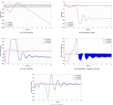
The simulated state responses and control effort for these angles of interest are given in Fig. 2 for the power series based controller and Fig. 3 for the LQR controller. The gray shaded region in Figs. 2a and 3a indicates the length of the track.

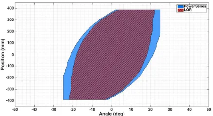
To get a better estimate of the stability region for the power series controller and the LQR controller, we repeat the simulations with various initial conditions for two of the states while keeping the initial condition for the other two states zero. The stability region estimates for initial conditions

−180◦ ≤ α0 ≤ 180◦, −590◦/s ≤ α˙0 ≤ 590◦/s, x0 = 0,

and x˙0 = 0 are given in Fig. 4, for initial conditions −180◦ ≤α0 ≤180◦, −390 mm ≤x0 ≤390 mm, x˙0 = 0,

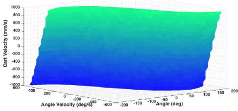
and α˙0 = 0 are given in Fig. 5, and for initial conditions −390 mm ≤ x0 ≤ 390 mm, −1000mm/s ≤ x˙0 ≤ 1000

mm/s, α0 = 0, and α˙0 = 0 are given in Fig. 6. The range

on the velocities was selected based on the values possible by the apparatus we use for real-time implementation, while the range on the cart’s position was selected to be within the length of the track. For all three cases, the stability region of the power series controller is bigger than the stability region of the LQR controller.

Finally, we repeat the simulations with various initial condi-tions for three of the states while keeping the initial condition for the remaining state zero. The stability region estimate for initial conditions −180◦ ≤ α0 ≤ 180◦, −590◦/s ≤ α˙0 ≤ 590◦/s, −1000 mm/s ≤ x˙0 ≤ 1000 mm/s, and x0 = 0 is

given in Fig. 7 for the power series based controller and in Fig. 8 for the LQR controller. The stability region estimate for initial conditions −180◦ ≤α0≤180◦,−590◦/s≤α˙0≤ 590◦/s, −390 mm ≤ x0 ≤ 390 mm, and x˙0 = 0 is given

in Fig. 9 for the power series based controller and in Fig. 10 for the LQR controller. The stability region of the power

series controller is bigger than the stability region of the LQR controller for both cases.

IV. REAL-TIMEIMPLEMENTATION

A. Apparatus

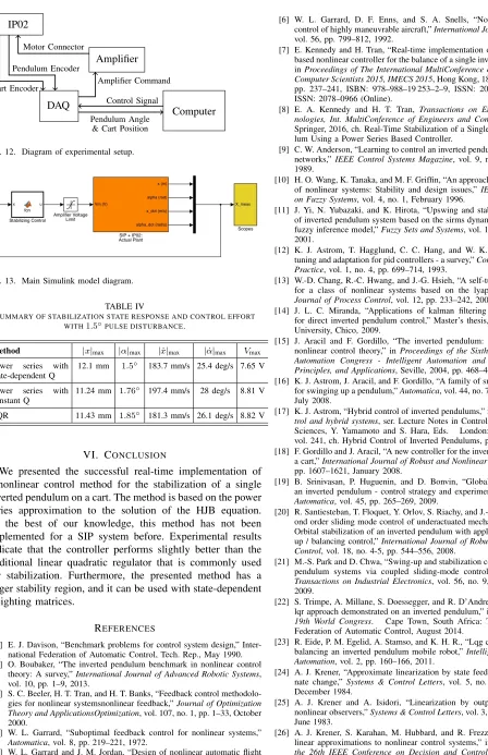
For our real-time experiments we use apparatus designed and provided by Quanser Consulting Inc. (119 Spy Court Markham, Ontario, L3R 5H6, Canada). This includes a single inverted pendulum mounted on an IP02 servo plant (depicted in Fig. 11), a VoltPAQ amplifier, and a Q2-USB DAQ con-trol board. The IP02 cart incorporates a Faulhaber Coreless DC Motor (2338S006) coupled with a Faulhaber Planetary Gearhead Series 23/1. The cart is also equipped with a US Digital S1 single-ended optical shaft encoder. The detailed technical specifications can be found in [41]. A diagram of our experimental setup is included in Fig. 12.

B. Design Specifications

The goal of our real-time experiment is to stabilize the inverted pendulum in the upright position with minimal cart movement and control effort. The weights Q(X) ≥ 0 and

R >0in the cost functional (9) must be chosen so that the sys-tem satisfies the following design performance requirements specified:

1) Regulate the pendulum angle around its upright position and never exceed a ±1-degree-deflection from it, i.e.

|α| ≤1.0◦.

2) Minimize the control effort produced, which is pro-portional to the motor input voltage Vm. The power amplifier should not go into saturation in any case, i.e.

|Vm| ≤10V.

C. MATLAB Implementation

Our Experimental results were obtained using Simulink in MATLAB and Quanser’s QuArc real-time control software. The diagram of the main Simulink model is given in Fig. 13. The control uis computed in real-time with a sampling rate of 1 kHz (1ms) using an Embedded Matlab Function block. The SIP+IP02 Actual Plant subsystem block that reads and computes the cart’s position and velocity, and the pendulum’s angle and angle velocity is taken from a model provided by Quanser.

V. EXPERIMENTALRESULTS

A. Constant Weighting Matrices

We have previously presented and discussed experimental results with constant weighting matricesQ(X) =QandRin [7], [8].

B. State-Dependent Weighting Matrix

The amount of time required for tuning the performance of the power series controller can be significantly reduced by using a state-dependent values in the weighting matrix

Q(X). The choice ofQ(X) =diag(800+5x2,150+2α2,1+ ˙

(6)

(a) Cart Position (b) Pendulum Angle

(c) Cart Velocity (d) Pendulum’s Angular Velocity

(e) Control Effort

Fig. 2. Simulated state response and control effort for the power series based controller with various initial angles, andx0= 0,α˙0= 0,x˙0= 0.

of the controller when compared to the performance of the other two control methods that just use the constant part of

Q(X), namely Q =diag(800,150,1,1). The corresponding state responses and control effort are provided in Fig. 14. A summary of the analysis of the state responses and the control effort for the three methods is provided in Tables II and III.

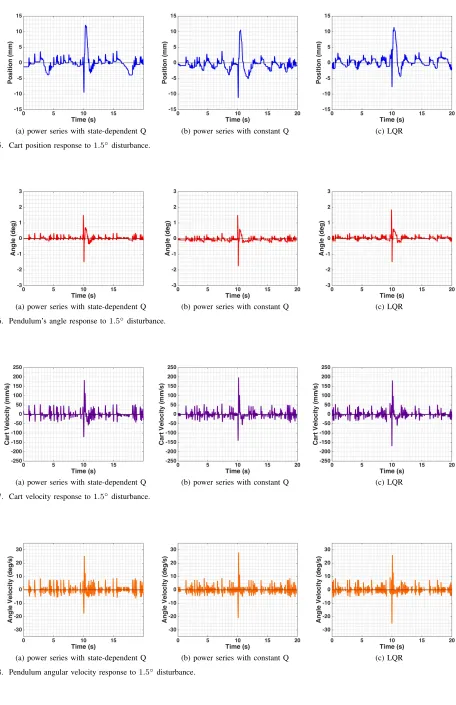
C. Disturbance Rejection

The performance of the power series based controller with both constant and state-dependent Q was compared to the performance of the LQR controller in response to a 1.5◦

angular pulse disturbance. A summary of the analysis of the state responses and the control effort for the three methods is provided in Table IV. Graphs of the corresponding state responses and control effort are provided in Figs. 15-19. The three controllers performed very similarly, but the power

TABLE II

SUMMARY OF STABILIZATION STATE RESPONSE FOR THE POWER SERIES BASED CONTROLLER WITH STATE-DEPENDENTQVS.CONTROLLERS WITH

Q=diag(800,150,1,1).

Method |x|max |α|max |x˙|max |α˙|max

|x|avg |α|avg |x˙|avg |α˙|avg

3.05 mm 0.176◦ 28.64 mm/s 3.53 deg/s power series with

state-dependent Q _{0.579 mm 2.67e-}₀₂◦ _{4.53 mm/s} _{0.765 deg/s}

3.8 mm 0.35◦ _{67.3 mm/s} _{10.73 deg/s}

power series with

constant Q _{0.775 mm 5.08e-}₀₂◦ _{7.35 mm/s} _{1.1 deg/s}

3.19 mm 0.264◦ _{60.6 mm/s} _{9.19 deg/s}

LQR

(7)

(e) Control Effort

Fig. 3. Simulated state response and control effort for the LQR controller with various initial angles, andx0= 0,α˙0= 0,x˙0= 0.

Fig. 4. Stability region estimate for both the power series based controller and the LQR controller for various initial pendulum angles and angular velocities with zero initial cart position and cart velocity.

(8)

Fig. 6. Stability region estimate for both the power series based controller and the LQR controller for various initial cart positions and cart velocities with zero initial pendulum angle and angular velocity.

Fig. 7. Stability region estimate for the power series based controller for various initial pendulum angles, angular velocities, and cart velocities with zero initial cart position.

Fig. 8. Stability region estimate for the LQR controller for various initial pendulum angles, angular velocities, and cart velocities with zero initial cart position.

TABLE III

SUMMARY OF STABILIZATION CONTROL EFFORT FOR THE POWER SERIES BASED CONTROLLER WITH STATE-DEPENDENTQVS.CONTROLLERS WITH

Q=diag(800,150,1,1).

Method Vmax |Vm|avg R₀30|Vm|dt

power series with state-dependent Q 1.82 V 0.358 V 10.73 V

power series with constant Q 2.9 V 0.41 V 12.33 V

LQR 2.59 V 0.392 V 11.77 V

Fig. 9. Stability region estimate for the power series based controller for various initial cart positions, pendulum angles, and angular velocities with zero initial cart velocity.

Fig. 10. Stability region estimate for the LQR controller for various initial cart positions, pendulum angles, and angular velocities with zero initial cart velocity.

Fig. 11. Single inverted pendulum mounted on a Quanser IP02 servo plant.

(9)

IP02 Amplifier DAQ Computer Control Signal Pendulum Angle & Cart Position Cart Encoder

Pendulum Encoder

Amplifier Command Motor Connector

Fig. 12. Diagram of experimental setup.

Fig. 13. Main Simulink model diagram.

TABLE IV

SUMMARY OF STABILIZATION STATE RESPONSE AND CONTROL EFFORT WITH1.5◦_{PULSE DISTURBANCE}_.

Method |x|max |α|max |x˙|max |α˙|max Vmax

power series with state-dependent Q

12.1 mm 1.5◦ 183.7 mm/s 25.4 deg/s 7.65 V

power series with constant Q

11.24 mm 1.76◦ _{197.4 mm/s} _{28 deg/s} _{8.81 V}

LQR 11.43 mm 1.85◦ 181.3 mm/s 26.1 deg/s 8.82 V

VI. CONCLUSION

We presented the successful real-time implementation of a nonlinear control method for the stabilization of a single inverted pendulum on a cart. The method is based on the power series approximation to the solution of the HJB equation. To the best of our knowledge, this method has not been implemented for a SIP system before. Experimental results indicate that the controller performs slightly better than the traditional linear quadratic regulator that is commonly used for stabilization. Furthermore, the presented method has a larger stability region, and it can be used with state-dependent weighting matrices.

REFERENCES

[1] E. J. Davison, “Benchmark problems for control system design,” Inter-national Federation of Automatic Control, Tech. Rep., May 1990. [2] O. Boubaker, “The inverted pendulum benchmark in nonlinear control

theory: A survey,”International Journal of Advanced Robotic Systems, vol. 10, pp. 1–9, 2013.

[3] S. C. Beeler, H. T. Tran, and H. T. Banks, “Feedback control methodolo-gies for nonlinear systemsnonlinear feedback,”Journal of Optimization Theory and ApplicationsOptimization, vol. 107, no. 1, pp. 1–33, October 2000.

[4] W. L. Garrard, “Suboptimal feedback control for nonlinear systems,” Automatica, vol. 8, pp. 219–221, 1972.

[5] W. L. Garrard and J. M. Jordan, “Design of nonlinear automatic flight control systems,”Automatica, vol. 13, pp. 497–505, 1977.

[6] W. L. Garrard, D. F. Enns, and S. A. Snells, “Nonlinear feedback control of highly maneuvrable aircraft,”International Journal of Control, vol. 56, pp. 799–812, 1992.

[7] E. Kennedy and H. Tran, “Real-time implementation of a power series based nonlinear controller for the balance of a single inverted pendulum,” inProceedings of The International MultiConference of Engineers and Computer Scientists 2015, IMECS 2015, Hong Kong, 18-20 March 2015, pp. 237–241, ISBN: 978–988–19 253–2–9, ISSN: 2078–0958 (Print); ISSN: 2078–0966 (Online).

[8] E. A. Kennedy and H. T. Tran, Transactions on Engineering Tech-nologies, Int. MultiConference of Engineers and Computer Scientists. Springer, 2016, ch. Real-Time Stabilization of a Single Inverted Pendu-lum Using a Power Series Based Controller.

[9] C. W. Anderson, “Learning to control an inverted pendulum using neural networks,”IEEE Control Systems Magazine, vol. 9, no. 3, pp. 31–37, 1989.

[10] H. O. Wang, K. Tanaka, and M. F. Griffin, “An approach to fuzzy control of nonlinear systems: Stability and design issues,”IEEE Transactions on Fuzzy Systems, vol. 4, no. 1, February 1996.

[11] J. Yi, N. Yubazaki, and K. Hirota, “Upswing and stabilization control of inverted pendulum system based on the sirms dynamically connected fuzzy inference model,”Fuzzy Sets and Systems, vol. 122, pp. 139–152, 2001.

[12] K. J. Astrom, T. Hagglund, C. C. Hang, and W. K. Ho, “Automatic tuning and adaptation for pid controllers - a survey,”Control Engineering Practice, vol. 1, no. 4, pp. 699–714, 1993.

[13] W.-D. Chang, R.-C. Hwang, and J.-G. Hsieh, “A self-tuning pid control for a class of nonlinear systems based on the lyapunov approach,” Journal of Process Control, vol. 12, pp. 233–242, 2002.

[14] J. L. C. Miranda, “Applications of kalman filtering and pid control for direct inverted pendulum control,” Master’s thesis, California State University, Chico, 2009.

[15] J. Aracil and F. Gordillo, “The inverted pendulum: A benchmark in nonlinear control theory,” inProceedings of the Sixth Biannual World Automation Congress - Intelligent Automation and Control Trends, Principles, and Applications, Seville, 2004, pp. 468–482.

[16] K. J. Astrom, J. Aracil, and F. Gordillo, “A family of smooth controllers for swinging up a pendulum,”Automatica, vol. 44, no. 7, pp. 1841–1848, July 2008.

[17] K. J. Astrom, “Hybrid control of inverted pendulums,” inLearning, con-trol and hybrid systems, ser. Lecture Notes in Control and Information Sciences, Y. Yamamoto and S. Hara, Eds. London: Springer, 1999, vol. 241, ch. Hybrid Control of Inverted Pendulums, pp. 150–163. [18] F. Gordillo and J. Aracil, “A new controller for the inverted pendulum on

a cart,”International Journal of Robust and Nonlinear Control, vol. 18, pp. 1607–1621, January 2008.

[19] B. Srinivasan, P. Huguenin, and D. Bonvin, “Global stabilization of an inverted pendulum - control strategy and experimental verification,” Automatica, vol. 45, pp. 265–269, 2009.

[20] R. Santiesteban, T. Floquet, Y. Orlov, S. Riachy, and J.-P. Richard, “Sec-ond order sliding mode control of underactuated mechanical systems ii: Orbital stabilization of an inverted pendulum with applications to swing up / balancing control,”International Journal of Robust and Nonlinear Control, vol. 18, no. 4-5, pp. 544–556, 2008.

[21] M.-S. Park and D. Chwa, “Swing-up and stabilization control of inverted pendulum systems via coupled sliding-mode control method,” IEEE Transactions on Industrial Electronics, vol. 56, no. 9, pp. 3541–3555, 2009.

[22] S. Trimpe, A. Millane, S. Doessegger, and R. D’Andrea, “A self-tuning lqr approach demonstrated on an inverted pendulum,” inPrepints of the 19th World Congress. Cape Town, South Africa: The International Federation of Automatic Control, August 2014.

[23] R. Eide, P. M. Egelid, A. Stamso, and K. H. R., “Lqg control design for balancing an inverted pendulum mobile robot,”Intelligent Control and Automation, vol. 2, pp. 160–166, 2011.

[24] A. J. Krener, “Approximate linearization by state feedback and coordi-nate change,” Systems & Control Letters, vol. 5, no. 3, pp. 181–185, December 1984.

[25] A. J. Krener and A. Isidori, “Linearization by output injection and nonlinear observers,”Systems & Control Letters, vol. 3, no. 1, pp. 47–52, June 1983.

(10)

(e) Control Effort

(11)

(a) power series with state-dependent Q (b) power series with constant Q (c) LQR

Fig. 15. Cart position response to1.5◦_disturbance.

Fig. 16. Pendulum’s angle response to1.5◦disturbance.

Fig. 17. Cart velocity response to1.5◦_disturbance.

(12)

Fig. 19. Control effort with1.5◦disturbance.

[27] L. R. Hunt and J. Turi, “A new algorithm for constructing approximate transformations for nonlinear systems,”IEEE Transactions on Automatic Control, vol. 38, no. 10, pp. 1553–1556, October 1993.

[28] A. Isidori,Nonlinear Control Systems. New York: Springer Verlag, 1989.

[29] T. Sugie and K. Fujimoto, “Control of inverted pendulum system based on approximate linearization: design and experiment,” inProceedings of the 33rd IEEE Conference on Decision & Control, vol. 2. Lake Buena Vista, FL: IEEE, December 1994, pp. 1647–1648.

[30] A. Ohsumi and T. Izumikawa, “Nonlinear control of swing-up and stabilization of an inverted pendulum,” inProceedings of the 34th IEEE Conference on Decision & Control. New Orleans, LA: IEEE, December 1995, pp. 3873–3880.

[31] L. Guzella and A. Isidori, “On approximate linearization of nonlinear control systems,”International Journal of Robust and Nonlinear Con-trol, vol. 3, no. 3, pp. 261–276, 1993.

[32] S. Renou and L. Saydy, “Real time control of an inverted pendulum based on approximate linearization,” inCanadian Conference on Elec-trical and Computer Engineering, vol. 2. Calgary, Alta: IEEE, May 1996, pp. 502–504.

[33] D. Ingram, S. S. Willson, P. Mullhaupt, and D. Bonvin, “Stabilization of an experimental cart-pendulum system through approximate manifold decomposition,” inPrepints of the 18th IFAC World Congress. Milano, Italy: International Federation of Automatic Control, 2011, pp. 10 659– 10 666.

[34] C. Huifeng, L. Hongxing, and Y. Peipei, “Swing-up and stabilization of the inverted pendulum by energy well and sdre,” in Control and Decision Conference, 2009. CCDC ’09. Chinese. IEEE, June 2009, pp. 2222–2226.

[35] N. M. Singh, J. Dubey, and G. Laddha, “Control of pendulum on a cart with state dependent riccati equations,”World Academy of Science, Engineering and Technology, vol. 2, no. 5, pp. 1283–1287, May 2008. [36] P. Dang and F. L. Lewis, “Controller for swing-up and balance of single inverted pendulum using sdre-based solution,” inIndustrial Electronics Society, 2005. IECON 2005. 31st Annual Conference of IEEE. IEEE, November 2005, pp. 304–309.

[37] S. A. Campbell, S. Crawford, and K. Morris, “Friction and the inverted pednulum stabilization problem,” Journal of Dynamic Systems, Mea-surement and Control, vol. 130, no. 5, September 2008.

[38] ——, “Time delay and feedback control of an inverted pendulum with stick slip friction,” inProceedings of ASME 2007 International Design Engineering Technical Conferences & Computers and Information in Engineering Conference, Las Vegas, September 2007.

[39] E. Kennedy, “Swing-up and stabilization of a single inverted pendulum: Real-time implementation,” Ph.D. dissertation, North Carolina State University, 2015. [Online]. Available: http://www.lib.ncsu.edu/resolver/ 1840.16/10416

[40] H. T. Banks, R. C. Smith, and Y. Wang, Smart Material Structures: Modeling, Estimation, and Control. Chichester, England: Wiley, 1996. [41] Linear Motion Servo Plants: IP01 or IP02 - IP01 and IP02 User

Manual, 5th ed., Quanser Consulting, Inc.

Emese Kennedy was born in Budapest, Hungary. She received the B.A. in mathematics from Skid-more College in 2010, and the M.S. and Ph.D. degrees in applied mathematics from North Carolina State University in 2013 and 2015, respectively. She is currently a Visiting Assistant Professor of Mathematics at Hollins University in Roanoke, VA.