A novel statistical analysis and interpretation of flow cytometry data

(1)

A Novel Statistical Analysis and Interpretation of Flow Cytometry

Data

H.T. Banks, D. F. Kapraun, and W. Clayton Thompson

Center for Research in Scientific Computation and Center for Quantitative Sciences in Biomedicine North Carolina State University, Raleigh, NC 27695-8212

Cristina Peligero, Jordi Argilaguet, and Andreas Meyerhans

ICREA Infection Biology Lab, Department of Experimental and Health Sciences Universitat Pompeu Fabra, 08003 Barcelona, Spain

March 31, 2013

Abstract

A recently developed class of models incorporating the cyton model of population generation structure into a conservation-based model of intracellular label dynamics is reviewed. Statistical aspects of the data collection process are quantified and incorporated into a parameter estimation scheme. This scheme is then applied to experimental data for PHA-stimulated CD4+ T and CD8+ T cells collected from two healthy donors. This novel mathematical and statistical framework is shown to form the basis for accurate, meaningful analysis of cellular behavior for a population of cells labeled with the dye CFSE and stimulated to divide.

1 Introduction

Dating at least as far back as the work of Bell and Anderson [14] in 1967, mathematical models have been proposed which attempt to describe the biophysical processes involved in cell division. These models range in scope and scale from phenomenological descriptions of population growth to mechanistic models of subcellular mechanics. One particularly important class of mathematical models is that in which the behaviors of individual cells are linked in a meaningful way to population level characteristics. This class of models has applications in quantitative descriptions of the immune system, where the behavior of individual cells can vary widely across the population but in which the immune response (understood to be the net result of actions of all relevant cells in the system) is much more predictable [43]. In fact, a quantitative description of the ‘cellular calculus’ [25] by which cells send, receive, and respond to intra- and extracellular stimuli is in many respects an open problem in immunology.

In the past, the major limitation of mathematical models linking cellular and population-level behavior has

been the difficulty in obtaining data with which to validate the models. Generally, it is possible to observe the

behavior of a small number of single cells quite carefully in isolation, or to observe a large number of cells in aggregate. More recently, the intracellular dye carboxyfluorescein succinimidyl ester (CFSE) [37] for use in flow-cytometric proliferation assays in vitro has emerged as a powerful experimental technique for the study of dividing cells. Because the dye emits bright, approximately uniform, and long-lasting fluorescent labeling of a population of cells and is approximately evenly partitioned during cell division, the dye provides a useful surrogate for the number of divisions a cell has undergone. Individual cells can be assessed by a flow cytometer, which can simultaneously measure additional properties of cells such as size, internal complexity, cell surface marker expression, levels of cytokine secretion, etc.

(2)

completed the same number of divisions. When such measurements are made sequentially in time, one obtains information on the dynamic response of the population of cells to a stimulus. As such, CFSE-based flow cytometric analysis is a promising tool for the study of cell division and division-linked changes. The ultimate goal for the quantitative analysis of CFSE data (in particular, as it relates to studies of the immune system) is to incorporate fundamental mechanistic modeling of the cellular calculus into a description of population-level behavior, and thus to obtain a more comprehensive understanding of the immune system, with obvious implications for the study of disease detection, progression, treatment/control, etc. To that end, mathematical modeling provides a quantitative framework with which to analyze and interpret such data.

A large number of mathematical models (see, e.g., the recent reviews [10, 38]) have been proposed with the aim of linking the generation structure (cells per number of divisions undergone) to quantitative descriptions of cellular behavior (e.g., times to division and death). Most recently [9], a class of mathematical models has been proposed which incorporates the ‘cyton’ model [28, 29] of cell division dynamics into a mathematical description of flow cytometry histogram data based upon conservation principles. Here, we revisit this new class of models and provide a more complete discussion of some mathematical properties of the solutions which make them amenable to the fast computational approaches as described in [27]. It is also shown how the new model can be compared with older label-structured models such as those proposed in [12, 27, 42, 47]. Next the data collection process is considered in more detail and a theoretical statistical model is derived. The mathematical and statistical models are then incorporated into a rigorous parameter estimation scheme based upon a weighted least squares framework and members of the proposed class of mathematical models are compared in terms of their ability to fit the available data.

2 CFSE Data

CFSE-based flow cytometry experiments are performed by stimulating CFSE-labeled cells to divide by exposure to either a mitogenic compound or a specific antigen. Cells are then placed into separate wells, one for each measurement to be made. Several protocols exist and can be tailored to the needs of a particular experiment. See, e.g., [36, 37, 41, 49, 51]. For the experiment described here, peripheral blood mononuclear cells (PBMCs) from two healthy donors were stained with CFSE and stimulated with the mitogen phytohaemagglutinin (PHA). Measurements were carried out approximately every 24 hours for five days, beginning one day after stimulation. When a well is selected for measurement, cells are additionally labeled for phenotypic identification by anti-bodies (anti-CD3 T, anti-CD4 T , and anti-CD8 T cells) tagged with fluorescent markers. These cells are then analyzed by flow cytometry, which records the relative brightness of cells in various colors (corresponding to distinct fluorescent markers). Cells of interest can then be identified in the flow cytometry output. For this experiment, we consider CD4 T cells (CD3+, CD4+, CD8-) and CD8 T cells (CD3+, CD4-, CD8+). Once these cells are identified, the fluorescence intensity (in the color channel consistent with CFSE) is analyzed for each cell. Because dead cells will disintegrate shortly after death and can be excluded by gating, mainly viable cells are measured by the flow cytometer (the fraction of cells which are dead but not yet disintegrated is assumed to be small).

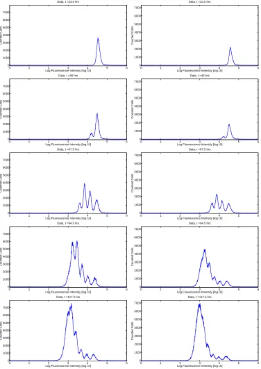
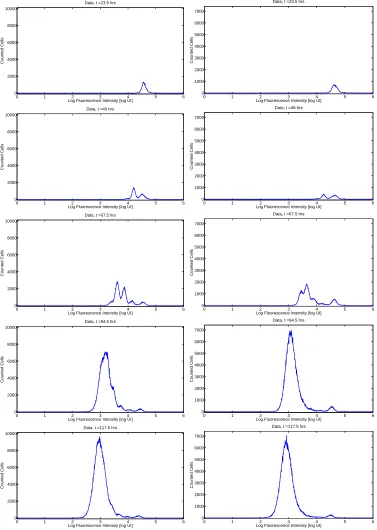
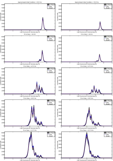
The population generation structure of the cells at a given measurement time can be visualized by organizing the fluorescence intensity measurements of individual cells into a histogram, as shown in Figures 1 and 2. Because of physical limitations, only a fraction of the cells contained in a selected well are actually analyzed by flow cytometry. In order to estimate the total number of cells in the measurement sample, a known number of fluorescent beads are placed in each sample; these beads can be identified and counted in the flow cytometry output and the ratio of beads counted to total beads introduced provides an estimate of the fraction of the sample acquired by the flow cytometer. The histogram profiles obtained from the measured cells can then be normalized by the reciprocal of this quantity.

(3)

0 1 2 3 4 5 6 0 1000 2000 3000 4000 5000 6000 7000

Data, t =23.5 hrs

Log Fluorescence Intensity [log UI]

Counted Cells

0 1 2 3 4 5 6

0 1000 2000 3000 4000 5000 6000 7000

Data, t =23.5 hrs

Counted Cells

0 1 2 3 4 5 6

0 1000 2000 3000 4000 5000 6000 7000

Data, t =46 hrs

Counted Cells

0 1 2 3 4 5 6

0 1000 2000 3000 4000 5000 6000 7000

Data, t =46 hrs

Counted Cells

0 1 2 3 4 5 6

0 1000 2000 3000 4000 5000 6000 7000

Data, t =67.5 hrs

Counted Cells

0 1 2 3 4 5 6

0 1000 2000 3000 4000 5000 6000 7000

Data, t =67.5 hrs

Counted Cells

0 1 2 3 4 5 6

0 1000 2000 3000 4000 5000 6000 7000

Data, t =94.5 hrs

Counted Cells

0 1 2 3 4 5 6

0 1000 2000 3000 4000 5000 6000 7000

Data, t =94.5 hrs

Counted Cells

0 1 2 3 4 5 6

0 1000 2000 3000 4000 5000 6000 7000

Data, t =117.5 hrs

Counted Cells

0 1 2 3 4 5 6

0 1000 2000 3000 4000 5000 6000 7000

Data, t =117.5 hrs

Counted Cells

(4)

0 1 2 3 4 5 6 0 2000 4000 6000 8000 10000

Data, t =23.5 hrs

Counted Cells

0 1 2 3 4 5 6

0 1000 2000 3000 4000 5000 6000 7000

Data, t =23.5 hrs

Counted Cells

0 1 2 3 4 5 6

0 2000 4000 6000 8000 10000

Data, t =46 hrs

Counted Cells

0 1 2 3 4 5 6

0 1000 2000 3000 4000 5000 6000 7000

Data, t =46 hrs

Counted Cells

0 1 2 3 4 5 6

0 2000 4000 6000 8000 10000

Data, t =67.5 hrs

Counted Cells

0 1 2 3 4 5 6

0 1000 2000 3000 4000 5000 6000 7000

Data, t =67.5 hrs

Counted Cells

0 1 2 3 4 5 6

0 2000 4000 6000 8000 10000

Data, t =94.5 hrs

Counted Cells

0 1 2 3 4 5 6

0 1000 2000 3000 4000 5000 6000 7000

Data, t =94.5 hrs

Counted Cells

0 1 2 3 4 5 6

0 2000 4000 6000 8000 10000

Data, t =117.5 hrs

Counted Cells

0 1 2 3 4 5 6

0 1000 2000 3000 4000 5000 6000 7000

Data, t =117.5 hrs

Counted Cells

(5)

A complete discussion of the mathematically relevant aspects of the data collection procedure can be found in [10]. The goal of the mathematical modeling process is to link a mathematical description of cellular division and death processes at the population level to the observed fluorescence intensity profiles as measured by a flow cytometer (Figures 1 and 2). Because each peak in the flow cytometry data represents a cohort of cells having completed the same number of divisions, it is hypothesized that flow cytometry data collected sequentially in time for cells from a single donor will contain sufficient information to analyze the dynamic response of those cells to stimulus. This dynamic response can only be accurately understood in the context of a mathematical

model of the biological system, as well as astatistical model linking the mathematical modelto the data. Such a

model must be able to account for the slow natural loss of CFSE fluorescence intensity over time, the dilution of fluorescence intensity by division, and the asynchronous nature of cellular division and death processes.

3 Mathematical Modeling of CFSE Data

We begin by summarizing a partial differential equation model structured by (continuous) fluorescence intensity and (discrete) division number which has been proposed to describe histogram data from CFSE-based proliferation assays [12, 27, 42, 47]. We then summarize a new class of models incorporating cyton dynamics into a label-structured framework and consider several different versions of the cyton model at greater length. Finally, the role of cellular autofluorescence is briefly considered.

3.1 Previous Label-Structured Model

Letni(t, x) be the structured density (cells per unit of fluorescence intensity) of a cohort of cells having completed

i_≥0 divisions at time tand withxunits of fluorescence intensityresulting from induced CFSE (that is, ignoring

the contributions of cellular autofluorescence). It is assumed that this fluorescence is directly proportional to the mass of CFSE within a cell, and thus can be treated as a mass-like quantity. These cells are assumed to divide

with time-dependent exponential rateαi(t) and die with time-dependent exponential rateβi(t). Then the entire

population of cells can be described by the system of partial differential equations

∂n0(t, x)

∂t −v(t)

∂[xn0(t, x)]

∂x =−(α0(t) +β0(t))n0(t, x)

∂n1(t, x)

∂t −v(t)

∂[xn1(t, x)]

∂x =−(α1(t) +β1(t))n1(t, x) +R1(t, x) (3.1)

.. .

The recruitment terms describe the symmetric division of CFSE upon mitosis and are given by Ri(t, x) =

4αi−1(t)ni−1(t,2x) for i ≥ 1; the form of these recruitment terms arises naturally from the derivation of the

above system of equations from conservation principles [47]. The advection term describes the rate of loss of fluo-rescence intensity (resulting from the turnover of CFSE), which is assumed to depend linearly on the fluofluo-rescence

intensityxwith time-dependent rate functionv(t). This follows the convention of [27], and includes exponential

loss (v(t) =c) and Gompertz decay (v(t) =ce−kt_{) as special cases. The loss of CFSE has been observed to be}

very rapid during the first 24 hours after initial labeling and much slower thereafter [12, 47]). Thus when data is collected in the first 24 hours, it is more accurate [7] to describe the rate of loss of fluorescence intensity with a time-varying rate (e.g., Gompertz decay). Such rates are consistent with the sequence of chemical reactions known to occur during the labeling process [18]. If data is not collected in the first day after labeling with CFSE (as in the data collected for this report) then, as we shall see below, exponential decay is sufficient. For the

remainder of this report, we assumev(t) =c.

The initial conditions for the model (3.1) are

ni(t0, x) =

Φ(x), i= 0

0, i_≥1 , (3.2)

forx≥0. Note that a no-flux condition atx= 0 is naturally satisfied by the form of the advection term provided

(6)

computed by the method of characteristics [47]. Alternatively, the following characterization of the solution is given in [42].

Proposition 3.1. The solution to (3.1)can be factored as

ni(t, x) =Ni(t)¯ni(t, x).

The functions Ni(t) indicate the number of cells having completed i divisions at time t and satisfy the weakly coupled system of ordinary differential equations

dN0(t)

dt =−(α0(t) +β0(t))N0(t)

dN1(t)

dt =−(α1(t) +β1(t))N1(t) + 2α0(t)N0(t)

..

. (3.3)

dNi(t)

dt =−(αi(t) +βi(t))Ni(t) + 2αi−1(t)Ni−1(t)

.. .

with initial conditions N0(t0) =N0,Ni(t0) = 0 for all i≥1. The functions ¯ni(t, x), describe the distribution of CFSE within a generation of cells. Each satisfies the equation

∂n¯i(t, x)

∂t −v(t)

∂[xn¯i(t, x)]

∂x = 0 (3.4)

for x_≥0 with initial condition

¯

ni(t0, x) =

2i_Φ(2i_x₎

N0

.

Again, the no flux condition at x = 0 is trivially satisfied by the form of the advection term. Note that, by definition,

N0=

Z ∞

0

Φ(x)dx.

We remark that the form of the equations presented above is slightly different from that considered in [12] as here we initially neglect considerations of autofluorescence. The formulation above follows the work of [27] and allows for a more intuitive formulation of the model, as well as the fast numerical techniques discussed below

and in the appendix. The system above is derived in terms of the fluorescence intensity resulting only from

induced CFSE; the experimentally measured fluorescence intensity is the sum of this quantity and the cellular

autofluorescencewhich results from the light absorption and emission properties of intracellular molecules. Let ˜

ni(t,x˜) be a structured density for cells having completedidivisions at timetwithmeasuredfluorescence intensity

˜

x. While the measured fluorescence intensity ˜xis given by the sum of the induced fluorescencexand the cellular

autofluorescence, this latter quantity may vary from cell to cell in the population. As such, given the solutions

ni(t, x) fori≥0 to (3.1), one computes the densities ˜ni(t,x˜) using the convolution integral [27, 42]

˜

ni(t,x˜) =

Z ∞

−∞

ni(t, x)p(t,x˜−x)dx=

Z x˜

0

ni(t, x)p(t,x˜−x)dx, (3.5)

wherep(t, ξ) is (for fixed time t) a probability density function describing the distribution of autofluorescence in

(7)

3.2 New Class of Label-Structured Models

While the model (3.1) for computing population label structure has been shown to accurately fit experimental data [12], it lacks a certain intuitive appeal in that the ‘time-dependent exponential rates’ of division and death,

αi(t) andβi(t), are not explained in biologically relevant terms (e.g., times to division and death). An alternative

to the mathematical model (3.3) is the cyton model for division dynamics [28, 29] which relates the number of cells in a population directly to probability distributions describing times at which cells divide or die. The cyton model is motivated by the assumption of independent regulation by the cellular machinery of times to division

and death. Using the definition ofNi(t) above, the cyton model is described by the set of equations

N0(t) =N0−

Z t

t0

ndiv0 (s) +ndie0 (s)

ds,

N1(t) =

Z t

t0

2ndiv0 (s)−n1div(s)−ndie1 (s)

ds, (3.6)

.. .

wherendiv

i (t) andndiei (t) indicate the rates (cells per hour) at which cells (having already undergoneidivisions)

divide and die, respectively, at time t. For undivided cells, let φ0(t) andψ0(t) be probability density functions

describing the distribution from which the times to division and death, respectively, are drawn. LetF0, called the

initial precursor fraction, be the fraction of undivided cells which would hypothetically divide in the absence of any cell death. (It is assumed that in each generation, non-progressing cells may die according to the probability

density functionψi(t), but may not divide.) Then, under the assumptions of the cyton model, it follows that

ndiv0 (t) =F0N0

1₋

Z t

t0

ψ0(s)ds

φ0(t),

ndie0 (t) =N0

1₋F0

Z t

t0

φ0(s)ds

ψ0(t). (3.7)

Similarly, one can define probability density functions φi(t) andψi(t) for times to division and death (measured

in hours since completion of the (i₋1)thdivision/death), respectively, for cells having undergoneidivisions, as

well as the progressor fractions Fi of cells which would complete the ith division in the absence of cell death.

Then the cell division and death rates are computed as

ndivi (t) = 2Fi

Z t

t0

ndivi−1(s)

1−

Z t−s

0

ψi(ξ)dξ

φi(t−s)ds,

ndiei (t) = 2

Z t

t0

ndivi−1(s)

1₋Fi

Z t−s

0

φi(ξ)dξ

ψi(t−s)ds. (3.8)

Given the success of the cyton model in describing cell dynamics, as well as the experimental evidence supporting it [10, 28, 29], the cyton model has been incorporated into a label-structured framework [9] similar to (3.1). The mathematical ideas rely heavily upon the separability of the model solution (Proposition 3.1) originally

demonstrated by [27, 42]. Letni(t, x) be a structured density as before. Consider the system of partial differential

equations

∂n0

∂t −v(t)

∂[xn0]

∂x =− n

div

0 (t) +ndie0 (t)

¯

n0(t, x)

∂n1

∂t −v(t)

∂[xn1]

∂x = 2n

div

0 (t)−ndiv1 (t)−ndie1 (t)

¯

n1(t, x) (3.9)

.. .

with initial conditions specified as for equation (3.1). The terms ¯ni(t, x) are described as in (3.4). This system of

(8)

for use with histogram data. We remark that (3.9) corrects a typographical error in [9], where the factors ¯ni(t, x)

were missing from the right side of the equations.

Proposition 3.2. The solution of (3.9)is

ni(t, x) =Ni(t)¯ni(t, x)

where the quantities Ni(t)satisfy (3.6)andn¯i(t, x)satisfy (3.4).

Proof. The proof follows immediately by the direct substitution of the stated solution into (3.9). Working with

the left side of (3.9) for the ith _equation,

∂ni(t, x)

∂t −v(t)

∂[xni(t, x)]

∂x =

∂[Ni(t)¯ni(t, x)]

∂t −v(t)

∂[xNi(t)¯ni(t, x)]

∂x

= dNi(t)

dt ¯ni(t, x) +Ni(t)

_∂_n_¯

i(t, x)

∂t −v(t)

∂[xn¯i(t, x)]

∂x

= 2ndivi−1−ndivi −ndiei

¯

ni(t, x),

which is exactly the right side of (3.9). For the purposes of this proof, it is assumed that ndiv

−1 = 0 so that the

equations for n0(t, x) are well-defined. It is easy to check that the initial and boundary conditions for (3.9) are

satisfied by the above solution.

Given the densities ni(t, x) computed according to (3.9), one can compute the densities ˜ni(t,x˜) via the

convolution (3.5) as before. Much like the original model (3.1), the new model (3.9) can be fit directly to histogram data from CFSE-based experiments and is highly accurate [9]. Significantly, the new model describes the dynamics of a dividing population of cells in intuitive terms (i.e., probability distributions of times to divide and die). This is the primary advantage of the new class of models over the previous modeling framework.

Similarly, while the cyton model has been widely used to analyze cell count dataobtained from CFSE data (e.g.,

through a deconvolution process; see [10]), the new class of models can be fit directly to CFSE histogram data.

As a result, the class of models is less dependent upon peak separation or a high frequency of cells which respond to stimulus. Moreover, the fit of the model to data can be assessed in a statistically rigorous manner (see Section 4 below).

Although the motivation for this model formulation is clear (combining cyton and label dynamics in a division-dependent compartmental model) the form of the new model is complex, describing the population densities

ni(t, x) in terms of yet another set of density functions, ¯ni(t, x). A simple reformulation shows that the new class

of models is consistent with the mass-conservation principles of the old label-structured model. Moreover, this reformulation shows how the two model forms can be related and directly compared.

Recall the definitions ofni(t, x),Ni(t), and ¯ni(t, x) given in Proposition 3.2. Note that

Z ∞

0

ni(t, x)dx=Ni(t),

and

Z ∞

0

¯

n(t, x)dx=

Z ∞

0

ni(t, x)

Ni(t)

dx= 1

Ni(t)

Z ∞

0

ni(t, x)dx= 1.

Thus the quantities ¯ni(t, x) can be considered as probability density functions for the distribution of CFSE in

cells having divided i times at time t. When considering cell death, the mathematical terms ndie

i (t)¯ni(t, x) in

(3.9) reflect the tacit assumption that the rate at which cells die (ndie

i (t)) is independent of the label distribution

¯

ni(t, x) of those cells. Moreover,

ndiei (t)¯ni(t, x) =ndiei (t)

ni(t, x)

Ni(t)

=n

die i (t)

Ni(t)

ni(t, x)

(9)

with

βi(t) =

ndie

i (t)

Ni(t)

, (3.10)

which is exactly the same form as (3.1). Similar statements hold true for the rates of dividing cells and the terms

αi(t) in Equation (3.1) if Fi of (3.7)-(3.8) equal 1 for all i. For 0 < Fi <1, then this is a more complex issue

and indeed is the subject of some of our current efforts. This fact can be used as the basis for a quantitative

comparison of the two model formulations, as well as to give physical/biological meaning to the time dependent exponential rates αi(t)andβi(t) used previously to describe cell division and death.

3.3 The Cyton Class of Models

It follows from the form of the equations (3.6)–(3.9) that the generation structure of the population (cells per

division number) is completely determined by the functionsφi(t) and ψi(t) and the progressor fractions Fi. To

motivate the form of the functions φi(t) andψi(t), define the random variableTidiv to be the time required for a

progressing cell to complete theith_{division, with the clock starting from the completion of the (}_i

−1)th _division.

(That is, the random variablesTdiv

i are defined in the temporal reference frames of the individual cells.) Similarly,

define the random variables Tdie

i to be the time required for a newly divided cell to die. The cyton model is

built from the premise that these two random variables are independent. Upon the completion of theith_division

(or upon activation, fori= 0), every cell realizes a new value for Tdiv

i andTidie; whichever realization is smaller

determines the eventual fate of the cell. The functions φi(t) and ψi(t) are the probability density functions for

Tdiv

i andTidie, respectively (which are assumed to be common for all cells having completedi divisions).

Experimental evidence suggests that the functionsφi(t) andψi(t) can be heuristically described by lognormal

probability density functions [28, 29]. Thus for allt >0,

φi(t) =

1

tσdiv

i

√

2πexp

−(logt−µ

div i )2

2(σdiv

i )2

,

ψi(t) = 1

tσdie

i

√

2πexp

−(logt−µ

die i )2

2(σdie

i )2

, (3.11)

where the parameters µdiv

i and σdivi represent the means and standard deviations of the natural logarithms of

the random variablesTdiv

i (and similarly forTidie). Since it is more intuitive to discuss the means and standard

deviations of the random variablesTdiv

i and Tidie directly (as opposed to the means and standard deviations of

their logarithms) these quantities are easily defined in terms of the parametersµdiv

i , µdiei ,σidiv, andσdiei :

E[Tdiv

i ] = exp

µdiv

i +

(σdiv

i )2

2

E[Tdie

i ] = exp

µdie

i +

(σdie

i )2

2

V ar[Tidiv] = exp (σidiv)2

−1

exp 2µdivi + (σdivi )2

V ar[Tidie] = exp (σidie)2

−1

exp 2µdiei + (σidie)2

.

For the basic cyton model, it is standard (following the work [28, 29]) to assume that the random variables

Tdiv

i are identically distributed for alli≥1 and that the random variablesTidie are identically distributed for all

i≥1. These distributions may be different from the corresponding random variables for undivided cells (i= 0).

Thus

µdivi =µdiv, i≥1

σidiv =σdiv, i≥1

µdiei =µdie, i≥1

(10)

It is also assumed thatFi = 1 for alli≥1 in the basic cyton model.

Of course, any number of generalizations of the basic cyton model is possible. For instance, following [28], the

fractions Fi can be defined in terms of adivision destiny. Among the cells which are activated to divide (F0N0

of them), let pi be the probability that a cell (or its progeny) ceases to be activated after completingidivisions

and define the cumulative probabilities

ci=

i

X

j=1

pj.

(Note that we must haveci→1 asi→ ∞.) It follows that the progressor fractions (fori≥1) are

Fi=

1−ci

1−ci−1

, ci−1<1

0, ci−1= 1. (3.12)

Rather than estimate the progressor fractions Fi (or the probabilities pi) independently, we follow the approach

suggested in [28] and assume that the probabilities pi can be described as a discrete normal density function

defined on the nonnegative integers. Thus the values of the probabilities pi (and the progressor fractions Fi)

are uniquely determined by the meanDµ and the standard deviationDσ of a discrete normal distribution. This

assumption has been shown to be consistent with experimental data [28] and has the beneficial effect of reducing the total number of parameters of the mathematical model.

We can now define the division destinies in terms of the progressor fractions (3.12). The division destiny

di is defined to be the fraction of cells out of those cells in the original population which would have proceeded

through exactlyidivisions in the absence of any cell death. These quantities are computed as

di=

1₋F0, i= 0

F0pi, i≥1. (3.13)

It should be noted that this definition does not make any assumptions regarding the exact lineage of cells (which cannot be determined from flow cytometry data) so that the progeny of a single cell are not assumed to all undergo the same number of divisions. Rather, one can consider a fractional number of precursors. For example, consider a single cell which divides once, after which one of the two daughter cells divides again. Then there are three

cells in the total population, and the division destinies are d0= 0,d1= 1/3,d2= 2/3. Though counterintuitive

for a single cell, division destinies provide an indication of the number of divisions undergone averaged over the

population of precursors.

Following the work presented in [9], one may also generalize the death rate mechanism for undivided cells to incorporate a separate set of behaviors for unactivated cells. In particular, it can be assumed that a fraction

pd of such cells will remain dormant and neither divide nor die during the experiment. The remaining fraction

(1₋pd) will die with some exponential rate β which is independent of the death-rate distribution of activated

cells. It follows that the probability density function describing cell death for undivided cells is

ψ0(t) = F0

tσdie

0

√

2πexp

−(logt−µ

die

0 )2

2(σdie

0 )2

+ (1−pd)(1−F0)βe−βt. (3.14)

It should be noted that this generalization changes the interpretation of the random variable Tdie

0 and its

rela-tionship to the parametersµdie

0 andσdie0 in the sense that the parametersµdie0 andσdie0 describe the statistical

properties of progressing cells only.

While the more complex death rate function (3.14) was found to accurately describe a CFSE data set in [9], the data sets collected for this manuscript differ in that the first measurement was taken approximately 24 hours after stimulation by PHA (as opposed to immediately following stimulation). As a result, the initial condition for the mathematical model represents only those cells which have not died in the first 24 hours after stimulation. It seems reasonable to hypothesize that such cells are unlikely to die at subsequent measurement times. Thus

an additional possibility is ψ0(t) = 0 for all t. (Thisψ0(t) is not a proper probability density function, but is

sufficient to describe the intended behavior. Equivalently, one could assume the function ψ0(t) has a large mean

(11)

Model Description Parameters (cyton only)

Model 1 Basic cyton model; Equations (3.11),Fi= 1 for alli≥1 9

Model 2 Basic cyton model plus division destiny according to (3.12) 11

Model 3 Basic cyton model, but with equation (3.14) for undivided cell death 11

Model 4 Basic cyton model, but with no undivided cell death (ψ0(t) = 0) 7

Model 5 Combine models 2 and 3 13

Model 6 Combine models 2 and 4 9

Model 7 Model 1, but with equation (3.15) for undivided cell division 12

Table 1: List of the possible cyton model parameterizations considered in this report. These models are compared (in terms of their ability to describe experimental data sets) in Tables 3 and 4.

Finally, we consider one possible generalization of the density function for time-to-first-division for progressing cells. If there are multiple subpopulations (e.g., naive vs. memory cells) contained within the population under

study, the density φ0(t) may be multimodal. For simplicity, we consider a bimodal density function which is a

weighted sum of two lognormal distributions,

φ0(t) =

f

tσdiv

0,a

√

2πexp −

(logt₋µdiv

0,a)2

2(σdiv

0,a)2

!

+ 1−f

tσdiv

0,b

√

2πexp −

(logt₋µdiv

0,b)2

2(σdiv

0,b)2

!

, (3.15)

wheref ∈[0,1] is a weighting parameter.

The possible model parameterizations considered in this report are summarized in Table 1.

3.4 Distribution of Cellular Autofluorescence

To this point we have considered a class of models based on the cyton modeling framework which describe the dynamic population generation structure for dividing cells. This class of models has been incorporated into a label-structured partial differential equation model derived by considering the CFSE in a mass-conservation

framework. As discussed previously, once the structured densitiesni(t, x) (in terms of the fluorescencexresulting

from CFSE) have been constructed, these quantities must be related to the measured fluorescence intensity ˜x

(which includes the contribution of cellular autofluorescence) via the convolution (3.5). Autofluorescence is the result of the absorption and emission properties of molecules which are naturally found within all cells and is present even in the absence of an added fluorescent label. Mean autofluorescence is known to increase as cells are activated to divide [1], probably as a result of the production of additional intracellular components associated with increased metabolic activity within the cell. Thus the notation of (3.5) explicitly includes the time-dependence

of the autofluorescence density function, p(t, ξ). Because these intracellular molecules are partitioned among

daughter cells during cell division, the distribution of autofluorescence can be intuitively considered as a growth and fragmentation process, which is known to produce skew-right density functions such as the lognormal density function [26]. In fact, it has been shown [12] that the distribution of autofluorescence in the population can be well-approximated using a lognormal density function, and thus can be characterized by its mean and its variance. This observation has been used as the basis for approximation techniques to the convolution (3.5) [27].

To test the assumption of lognormality, a portion of PBMC cells from each donor were set aside and stimulated with PHA but never labeled with CFSE. Thus the measured fluorescence distribution of these cells (represented

in histogram form) can be used to approximate the density function p(t, ξ) representing the actual population

(12)

lognormal density functions from the autofluorescence data. The first method is the method of moments, in which the exact mean and variance of the measured cells was computed and a lognormal curve was constructed with the same mean and variance. (In the figures, the resulting lognormal density function has been scaled by the number of cells in the data to facilitate comparison.) The second method is to use least squares to estimate the scale, mean, and variance of a lognormal density function.

Though the autofluorescence data is not perfectly lognormal, the assumption is fairly accurate for both cell types and both donors. For CD4 T cells, the lognormal approximation becomes more accurate as time progresses. This is consistent with the existence of an initial transient distribution of autofluorescence which corresponds to the quiescent state of the cells at the start of the experiment; as cells are activated to divide, the lognormal (or at least skew-right) distribution emerges possibly as a result of growth and division processes [26]. For CD8 T cells, the validity of the approximation does not change much in time.

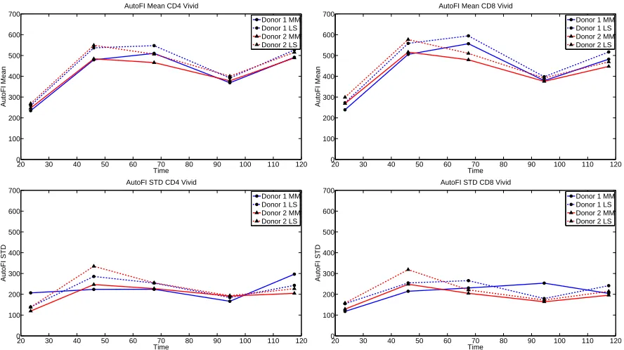
Significantly, the statistical moments of the autofluorescence distribution are observed to change in time (Figure 5). This is particularly true for the mean. The significant increase in mean autofluorescence between 24 and 48 hours is known to be associated with cellular activation. Though the increase is large, it is of little consequence for mathematical modeling because the contribution of autofluorescence to the fluorescence intensity measurements is very small (less than 1%) for undivided cells. The decrease in autofluorescence as measured

at approximately t= 96 hours is more problematic as some cells will have completed multiple divisions by that

time; the cause of the decrease is unknown. It is possible that a change in instrument settings between the two measurement days could account for this effect. Yet this seems unlikely as comparable changes are not observed in the data collected for cells labeled with CFSE (Figures 1 and 2). Another possibility is nutrient depletion; by the third day of the experiment, the cells begin to run out of the nutrients originally placed in culture and these must be replaced. Nutrient depletion could cause activated cells to die or return to a quiescent state.

Based upon these observations, the population distribution of autofluorescence can be accurately described as a lognormal density function at each measurement time. Thus

p(t, ξ) = 1

ξσxa(t)

√

2πexp

−(logξ−µxa(t))

2

2σxa(t)

2

, (3.16)

where the parameters µxa(t) andσxa(t) are related to the mean and standard deviation of the autofluorescence

distribution (at time t) by the formulas

µxa(t) = log(E[xa(t)])−

1

2log

1 + ST D(xa(t))

2

E[xa(t)]2

σx2a(t) = log

1 +ST D(xa(t))

2

E[xa(t)]2

.

In the context of parameter estimation for the mathematical model (3.9), we consider two frameworks.

The first is to use the method of moments (as above) with the autofluorescence data to compute E[xa(t)] and

ST D(xa(t)); these values will then be considered fixed while the remaining parameters of the mathematical model

are determined by using least squares to fit the data in Figures 1 and 2 (see Section 4 below). The second method

is to ignore the time-dependence of the distribution and assumeE[xa(t)] =E[xa],ST D(xa(t)) =ST D(xa). The

values of E[xa] and ST D(xa) are estimated in a least squares framework as described in Section 4, and these

estimated values can be compared to the values returned by the method of moments. One could also attempt to

parameterize and estimate a functionp(t, ξ) which is time-dependent. This is a more complex estimation problem

(13)

0 100 200 300 400 500 600 700 800 900 1000 0 50 100 150 200 250

AutoFI Distbn, DonorCP Vivid CD4 Day 1

AutoFI

Cell Counts

Data MM LS

0 100 200 300 400 500 600 700 800 900 1000 0 50 100 150 200 250

AutoFI Distbn, DonorJA Vivid CD4 Day 1

AutoFI

Cell Counts

Data MM LS

0 100 200 300 400 500 600 700 800 900 1000 0 50 100 150 200 250

AutoFI

Cell Counts

Data MM LS

0 100 200 300 400 500 600 700 800 900 1000 0 50 100 150 200 250

AutoFI

Cell Counts

Data MM LS

0 100 200 300 400 500 600 700 800 900 1000 0 50 100 150 200 250

AutoFI

Cell Counts

Data MM LS

0 100 200 300 400 500 600 700 800 900 1000 0 50 100 150 200 250

AutoFI

Cell Counts

Data MM LS

0 100 200 300 400 500 600 700 800 900 1000 0 50 100 150 200 250

AutoFI

Cell Counts

Data MM LS

0 100 200 300 400 500 600 700 800 900 1000 0 50 100 150 200 250

AutoFI

Cell Counts

Data MM LS

0 100 200 300 400 500 600 700 800 900 1000 0 50 100 150 200 250

AutoFI

Cell Counts

Data MM LS

0 100 200 300 400 500 600 700 800 900 1000 0 50 100 150 200 250

AutoFI

Cell Counts

Data MM LS

(14)

0 100 200 300 400 500 600 700 800 900 1000 0 50 100 150 200 250

AutoFI

Cell Counts

Data MM LS

0 100 200 300 400 500 600 700 800 900 1000 0 50 100 150 200 250

AutoFI

Cell Counts

Data MM LS

0 100 200 300 400 500 600 700 800 900 1000 0 50 100 150 200 250

AutoFI

Cell Counts

Data MM LS

0 100 200 300 400 500 600 700 800 900 1000 0 50 100 150 200 250

AutoFI

Cell Counts

Data MM LS

0 100 200 300 400 500 600 700 800 900 1000 0 50 100 150 200 250

AutoFI

Cell Counts

Data MM LS

0 100 200 300 400 500 600 700 800 900 1000 0 50 100 150 200 250

AutoFI

Cell Counts

Data MM LS

0 100 200 300 400 500 600 700 800 900 1000 0 50 100 150 200 250

AutoFI

Cell Counts

Data MM LS

0 100 200 300 400 500 600 700 800 900 1000 0 50 100 150 200 250

AutoFI

Cell Counts

Data MM LS

0 100 200 300 400 500 600 700 800 900 1000 0 50 100 150 200 250

AutoFI

Cell Counts

Data MM LS

0 100 200 300 400 500 600 700 800 900 1000 0 50 100 150 200 250

AutoFI

Cell Counts

Data MM LS

(15)

20 30 40 50 60 70 80 90 100 110 120 0

100 200 300 400 500 600 700

AutoFI Mean CD4 Vivid

Time

AutoFI Mean

Donor 1 MM Donor 1 LS Donor 2 MM Donor 2 LS

20 30 40 50 60 70 80 90 100 110 120

0 100 200 300 400 500 600 700

AutoFI Mean CD8 Vivid

Time

AutoFI Mean

20 30 40 50 60 70 80 90 100 110 120

0 100 200 300 400 500 600 700

AutoFI STD CD4 Vivid

Time

AutoFI STD

20 30 40 50 60 70 80 90 100 110 120

0 100 200 300 400 500 600 700

AutoFI STD CD8 Vivid

Time

AutoFI STD

(16)

4 Statistical Modeling of CFSE Data

Models similar to those discussed in Section 3 have previously been shown to accurately describe population generation structure as measured by flow cytometry [9]. However the statistical properties of the measurement process have not been nearly as carefully considered. A major limitation of the current modeling framework lies not in the mathematical model itself but rather in the statistical model which links the mathematical model to

the data. An accurate statistical model is of vital importance for theconsistent estimation of model parameters,

as well as the unbiased estimation of confidence intervals around those parameters [2, 13, 19, 45]. Additionally,

an accurate statistical model is necessary for the rigorous comparison of different model parameterizations and generalizations [3, 5, 16] and the optimal design of experiments [4].

To this point, we have discussed a class of mathematical models which combine the cyton modeling framework of [28, 29] with the label and division structured population models of [12, 27, 42, 47] to describe CFSE data. Given several members of this class of models (see, e.g., Table 1) there is a need to compare the mathematical models on a quantitative basis in order to identify which model provides the ‘best’ (in an appropriate sense) description of an underlying experimental data set. Several techniques based upon information theory [16] or asymptotic properties of least squares estimators [3, 5, 24] have been developed for this purpose. In all cases, the techniques are premised upon an accurate statistical model which links the mathematical model to the collected data.

Mathematical descriptions of CFSE data have generally described numbers of cells per generation asestimated

from histogram data, rather than the histogram data itself. As such, little consideration has been given to the statistical model which generates the histogram data. In their likelihood estimation framework, Hyrien and Zand [31] propose that the marginal probability density of each datum is normally distributed, and that the variance of this normal distribution is constant for all data points. Least squares estimators, though not restricted to any

parametric class of probability density functions, have also generally assumed a constant variance error model

[7, 8, 9, 12, 34, 35, 47]. However, it has been shown that such an assumption does not accurately describe the variance as observed in actual data sets [8, 12, 47]. Another common error model for least squares estimation, in which the variance of each data point is assumed to be directly proportional to the square of the model value

at that point (a constant coefficient of variance model) has also been hypothesized, but was again observed to

be inaccurate [8, 12, 47]. Here, we revisit the discussion of [47, Ch. 4] to consider the probabilistic aspects of the actual experimental process itself and derive a hypothetical statistical model from a theoretical basis. This statistical model is then incorporated into a weighted least squares estimation scheme and several computational algorithms are proposed.

4.1 Theoretical Statistical Model

Define the structured densities ˜ni(t,˜x) (in terms ofmeasured fluorescence intensity) for cells having completedi

divisions as in Section 3. Then the structured density for the entire population of cells is

˜

n(t,x˜) =X

i

˜

ni(t,x˜). (4.1)

Because CFSE histogram data are most commonly represented using a base 10 logarithmic scale, we define the

change of variablesz= log10(˜x) to arrive at

ˆ

n(t, z) = 10zlog(10)˜n(t,10z)

which gives the structured density (measured in cells per base 10 log unit intensity) for the entire population

of cells at time t. Let N_kj be a random variable representing the number of cells measured at time tj with

log-fluorescence intensity in the region [zk, zk+1). The goal of the statistical model is to link the structured density

ˆ

n(t, z) to the data random variablesNkjin a manner that is consistent with the statistical properties of the random

variablesN_kj. Moreover, in the experimental process, the quantities N_kj are not directly measured. Rather, only

(17)

output) are contained within each sample to be measured. By comparing the number of beads acquired to the number of beads known to be in the tube, one is able to estimate the fraction of the sample acquired.

Let~q be the vector of parameters of the mathematical model (that is, ~q contains the parameters necessary

to describe the cyton dynamics as well as the parameters describing the label loss functionv(t) and the

autofluo-rescence distributionp(t, ξ)) so that we may rewrite ˆn(t, z) = ˆn(t, z;~q). In order to derive an error model for the

histogram data we first make the common assumption that the model is correctly specified so that the structured

population density ˆn(t, z;~q0) (where ~q0 is a hypothetical ‘true’ parameter) perfectly describes the population of

cells. Let Ni(t) be defined as in (3.6) and letN(t) =PNi(t). That is,N(t) is the total number of cells in the

population at time t. Define

pj(z) =

ˆ

n(tj, z;~q0)

N(tj)

.

It follows thatpj(z) is a probability density function. LetSj be the number of cells of interest (e.g., CD4 T cells)

sampled at measurement timetj. Then one can consider the sample ofSj cells (of interest) to be taken without

replacement from the total population ofN(tj) cells; the fluorescence intensity of the sampled cells is subject to

the sampling density pj(z). It should be carefully noted that there are numerous steps required to separate the

cells of interest from the actual culture of cells passing through the cytometer. See, e.g., [10, Sec. 2]. References

to the total number of cellsN(t), and the number of sampled cellsSj are understood to refer only to the specific

cells of interest in the experiment. For the moment, we make the additional assumption that these two numbers are exact and are not subject to any errors (systematic, experimental, or otherwise) caused by gating, etc.

Let B be the total number of beads (in each sample tube) which are used to quantify the fraction of the

population of cells which is measured at time tj and letbj be the ‘true’ number of beads passing through the

cytometer. By this, we mean the exact number of beads whichwould pass through the cytometer if the measured

culture were perfectly homogeneous, etc. It follows that

Sj =

bj

BN(tj).

Now consider the kth _{histogram bin [}_z

k, zk+1). The number of cells in the whole population which are

contained in this bin is

I[ˆn](tj, zk;~q0) =

Z zk+1

zk

ˆ

n(tj, z;~q0)dz. (4.2)

Let M_kj be a random variable representing the number of cells (out of the sampled population) counted into

thekth _{bin. Because the measurement process represents a sampling without replacement, it follows that}_Mj

k is

described by a hypergeometric distribution,

M_kj_∼HypG(N(tj), I[ˆn](tj, zk;~q0), Sj).

That is, Sj cells are sampled without replacement from a population containing a total ofN(tj) cells, of which

I[ˆn](tj, zk;~q0) are of interest. We make the following assumptions regarding the measurement process:

• N(tj)>> Sj (and thusI[ˆn(tj, zk;~q0)]>> SjI[ˆn_N](₍tj_t_j,z₎k;~q0))

• 0< ǫ≤ I[ˆn(tj,zk;~q0)]

N(tj) ≤1−ǫ <1.

Then it can be shown [23] thatMkj

distbn

−−−−→M˜kj where

˜

M_kj_{∼ N}

_S

jI[ˆn](tj, zk;~q0)

N(tj)

,SjI[ˆn](tj, zk;~q0)

N(tj)

1₋I[ˆn](tj, zk;~q0)

N(tj)

=_N

_b

j

B

N(tj)I[ˆn](tj, zk;~q0)

N(tj)

,bj

B

N(tj)I[ˆn](tj, zk;~q0)

N(tj)

1₋I[ˆn](tj, zk;~q0)

N(tj)

≈ N

_b

j

BI[ˆn](tj, zk;~q0),

bj

BI[ˆn](tj, zk;~q0)

(18)

Notation Description ˆ

n(t, z) Log-transformed label structured density

N(t) Total number of cells in the population at timet

pj(z) Probability density function from which cells are sampled

Sj Number of cells sampled at timetj

B Total number of beads originally placed into each well

bj ‘True’ number of beads counted by the cytometer at timetj

I[ˆn](tj, zk;~q0) ‘True’ number of cells from the total population belonging in thekthhistogram bin at time

tj

M_kj Random variable representing the number of cells counted into the kth _{histogram bin at}

timetj

ˆ

bj Actual number of beads counted by the flow cytometer (a realization ofbj)

N_kj Random variable resulting whenM_kj is scaled by the ratioB/ˆbj

njk The actual data, a realization of Njk

λj Random variable representing the bead count error ratiobj/ˆbj

Table 2: Summary of notation for the statistical model.

The final approximation is valid providedI[ˆn](tj, zk;~q0)<< N(tj), which is a perfectly reasonable assumption.

It can easily be shown that the first assumption regarding the measurement process is accurate provided

bj/B << 1, which again is reasonable (the ratio is typically less than 0.1). This assumption is necessary to

ensure that the sampling (without replacement) process is conducted in a such a way that the ratio of cells of interest to total cells is approximately constant during the measurement. The assumption is unusual in that it places a restriction on the total amount of data which can be collected. The second assumption regarding the measurement process bounds the probability that a cell belongs to a particular bin away from zero and one (although this assumption is not strictly necessary in some cases [33]). In practice, this assumption is only violated

whenI[˜n(tj, zk;~q0)]≈0.

Finally, when the measurements are actually taken, a certain number of beads ˆbj are actually counted. We

would certainly hope that ˆbj ≈bj; however, we can think of ˆbjas a realization of some random variable (which may

or may not be an unbiased estimator of bj, depending upon any systematic error that might occur in obtaining

bead counts from flow cytometry data). To obtain the histogram data which is actually used to calibrate the

mathematical model, one scales the sampled cell countsM_kj by the inverse of the fraction of the total population

actually sampled (as estimated by the number of counted beads ˆbj). Thus the data may be represented by the

random variable

N_kj= B

ˆ_b_jM

j k.

It follows that

N_kj_{∼ N} B

ˆ

bj

BI[ˆn](tj, zk;~q0),

B2

ˆ_b2

j

bj

BI[ˆn](tj, zk;~q0)

!

=_N λjI[ˆn](tj, zk;~q0), λj

B ˆ

bj

I[ˆn](tj, zk;~q0)

!

, (4.3)

where we have defined λj = bj/ˆbj. The quantities λj in effect represent a ‘scaling error’ and are sufficient to

explain the apparent violation of conservation principles often noticed in flow cytometry data (see, e.g, [7, 20, 32]; the problem is discussed at greater length in [47, Chs. 1,4]).

(19)

with the magnitude of the model solution. This relationship has been shown to accurately describe CFSE data [5, 47], and we can use this relationship to establish a parameter estimation framework.

4.2 Parameter Estimation

The goal of the parameter estimation problem is to find an estimate for the parameter~q0 which is assumed to

generate the data (neglecting model misspecification). In the above statistical model, we must also estimate the

nuisance parameters~λ=_{λj}. Given a collection of random variablesNkjdistributed according to (4.3), one may

define theestimators

(~qW LS, ~λW LS) = arg min

(~q,~λ)∈Q×Λ

J((~q, ~λ)_|{N_kj_}) = arg min

(~q,~λ)∈Q×Λ

X

j,k

λjI[ˆn](tj, zk;~q)−N_kj

2

wj_k (4.4)

where the weights are chosen in a manner that accounts for the assumed reliability of each measurement (see

below). Experimental data is considered as a set of realizationsnj_k of the random variablesN_kj; these are used to

obtain theestimates

(ˆq,λˆ) = arg min

(~q,~λ)∈Q×Λ

J((~q, ~λ)_|{nj_k_}) = arg min

(~q,~λ)∈Q×Λ

X

j,k

λjI[ˆn](tj, zk;~q)−nj_k

2

w_kj . (4.5)

We see that the cost functional J, and thus the estimators, depends upon the data random variablesNkj and

thus on the statistical model (4.3). In order for the estimators ~qW LS and~λW LS to be asymptotically optimal,

the weightswj_k must be chosen to match the variance of the random variablesN_kj [44, 45],

wj_k=

(

λjˆ_bB_jI[ˆn](tj, zkj;q~0), I[n](tj, zkj;~q0)> I∗

λjˆB_b_jI

∗_, _I_[_n_](_t

j, zkj;~q0)≤I∗

. (4.6)

The cutoff valueI∗_>_{0 is determined by the experimenter so that the resulting residuals appear random. In the}

work that follows,I∗_{= 200. The values of}_B_{and ˆ}_b

j are known from the experiment. Notice that the computation

of the weights (4.6) depends upon the value of the ‘true’ parameter ~q0 as well as on the nuisance parameters~λ.

As a result, one must use an iterative estimation procedure [13, 19].

Traditionally, it has been assumed thatλj = 1 for allj [7, 8, 9, 12, 35]–that is, that there is no scaling error.

While this assumption is obviously violated by some data sets [7, 20, 32, 47] it is not clear that the incorpo-ration or omission of the nuisance parameters will have a significant effect on the estimation of parameters. In practice, the nuisance parameter vector must be estimated in conjunction with the model parameter vector in a two-stage process. Unfortunately two-stage estimation may cause some parameters of the mathematical model to become unidentifiable (or, at the very least, the variance of the estimators for certain parameters may increase

dramatically). For this report, it will be assumed that λj = 1 for all j and the nuisance parameters will not

be estimated. As will be seen in Section 5, the available data is well-described by the mathematical model even under this simplified assumption. We consider the following estimation algorithm:

1. Setℓ= 0. Obtain an initial estimate (the ordinary least squares estimate) by solving (4.5) with~λ= (1, . . . ,1)

andw_kj = 1 for allj andk,

ˆ

q(0)= arg min

~ q∈Q

X

j,k

I[ˆn](tj, zk;~q)−njk

2

;

2. Compute the weightswjk for eachjandkaccording to (4.6) with~q0replaced by ˆq(0)and with~λ= (1, . . . ,1);

(20)

4. Update the weights again according to (4.6), now with~q0replaced by ˆq(ℓ)(and~λ= (1, . . . ,1) still); increment

ℓ;

5. Repeat steps 3 and 4 until convergence is obtained.

5 Results

Twelve models of cyton dynamics are considered in Table 1 and two methods of estimating the statistical moments of the autofluorescence distribution(s) as proposed in Section 3.4 are used. In order to determine which of these model formulations best describes the available data, we need mathematical tools for rigorous model comparison. These tools are explored in Section 5.1 below and a best-fit model is selected. The fit of this model to the data, as well as the statistical model of the data, are then discussed. Finally, the dynamic responsiveness of the cells from the experimental data is analyzed.

5.1 Model Comparison

From Section 3.3, it is clear that some of the models of cyton dynamics are refinements of other models (in the sense that the more complex model includes all possible solutions of the simpler model). For instance, the basic

cyton model (Model 1) can be considered as a refinement of a cyton model for which it is assumed ψ0(t) = 0

(Model 6). This is because, for appropriate choices of the parametersE[Tdie

0 ] andST D[T0die], Model 1 is exactly

equivalent to Model 6. In such a case, it is clear that the more complex model must result in a minimized cost functional at least as low as that of the simpler model; yet the more complex model has more parameters, and one must consider the possibility of overparameterization against this decrease in the least squares cost. To this end, results from the asymptotic theory of least squares estimators can be extended [5] to weighted least squares estimators such as (4.4).

Assume (without loss of generality) that the nuisance parameters ~λ are known. Let~qW LS be defined, as

above, as the minimizer over the admissible parameter spaceQof the least squares cost functionJ((~q, ~λ)_|{N_kj_}).

Now define ˜qW LS to be the minimizer ofJ((~q, ~λ)|{N_kj}) over the restricted parameter setQH, whereQH={q∈

Q|Hq =h}for some linear function H of rankrand a vector hof sizer×1. (For nonlinear restrictions on the

parameter space, a locally equivalent condition can be derived from the first order linearization of the nonlinear constraint; see [5].) In such situations, the model comparison problem can be recast as one of hypothesis testing. Consider the null and alternative hypotheses,

H0: q∈QH

HA: q6∈QH.

Then under fairly general conditions (see [5]) and assuming the null hypothesis is true, the test statistic

Un =

nJ((˜qW LS, ~λ)|{Nkj})−J((~qW LS, ~λ)|{Nkj})

J((~qW LS, ~λ)|{Nkj})

(where n is the total number of data points) is asymptotically a chi-square random variable with r degrees of

freedom, Un ∼ χ2(r). Thus given the data {nj_k} as realizations of the random variables N_kj, one obtains a

realization un of Un which can be used to assess the likelihood that the decrease in cost associated with the

unrestricted parameter space is the result of chance (see [13, Sec. 3.5]). The complete conditions under whichUn

is asymptotically distributed as a chi-square random variable, as well as a proof of the result, can be found in [5] and the references therein.

For comparison among models which are not refinements, one can use information theoretic criteria such as Akaike’s Information Criterion (AIC). From (4.3), it follows that the scaled residuals

r_kj =λjI[ˆn](tj, zk;~q)−N

j k

q

wj_k

(21)

are independent and normally distributed with constant variance (for all kand j). Then the AIC, which is the expected value of the relative Kullback-Leibler distance for a given model [16], is

Kn=nlog

J((~qW LS, ~λ)|{N_kj})

n

!

+ 2p (5.2)

where pis the dimension of the space Qfor the particular model of interest. Because Kn provides information

regarding the relative Kullback-Leibler distance, AIC values have meaning only in comparison to one another.

The model which results in the lowest AIC value is the most likely model for the particular data set being investigated. We note that a direct comparison of the costs (in Tables 3 and 4) may not be reasonable due to

the fact that the AIC values also must take into account the numberpof parameters estimated in a given model

(see (5.2)). A derivation of the AIC as well as numerous examples can be found in [16].

With these tools, we are now ready to compare the models suggested in Sections 3.3 and 3.4. The minimized

costs J((ˆqW LS, ~λj)) for each donor, cell type, and model are summarized in Tables 3 and 4. Table 3 contains

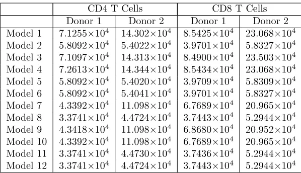
the results when the autofluorescence distribution is assumed to be time-invariant and its statistical moments are estimated within the least squares framework summarized in Section 4; Table 4 contains the results when the autofluorescence distribution is estimated at each measurement time using the method of moments.

CD4 T Cells CD8 T Cells

Donor 1 Donor 2 Donor 1 Donor 2

Model 1 6.0547_×104 _11.812

×104 _7.9383

×104 _20.348

×104

Model 2 5.4212_×104 _5.1257

×104 _2.8669

×104 _4.5650

×104

Model 3 6.0344×104 _11.812_×₁₀4 _8.2439_×₁₀4 _20.348_×₁₀4

Model 4 6.1677×104 _11.863_×₁₀4 _7.9383_×₁₀4 _20.348_×₁₀4

Model 5 5.4212×104 _5.1257_×₁₀4 _2.7963_×₁₀4 _4.5651_×₁₀4

Model 6 5.4212×104 _5.1257_×₁₀4 _2.8670_×₁₀4 _4.5650_×₁₀4

Model 7 4.3175×104 _9.4856_×₁₀4 _6.1827_×₁₀4 _18.761_×₁₀4

Model 8 3.4376×104 4.2341×104 2.8038×104 3.9553×104

Model 9 4.4006_×104 _9.5017

×104 _6.0628

×104 _19.563

×104

Model 10 4.3196_×104 _9.4931

×104 _6.2538

×104 _18.761

×104

Model 11 3.4375_×104 _4.2346

×104 _2.8004

×104 _3.9551

×104

Model 12 3.4376_×104 _4.8931

×104 _2.8038

×104 _3.9554

×104

Table 3: Minimized weighted least squares costs J((ˆq, ~λ)) for various cyton model parameterizations (see Table

1). Autofluorescence estimated as a time-invariant lognormal density function by least squares fit to data.

Of the 12 models of cyton dynamics considered, Model 12 is generally selected as the best model. The only exception is for Donor 2 CD4 T cells when estimating a time-invariant autofluorescence distribution using least

squares. In this case, Model 8 is narrowly selected by the AIC (K= 9525.77 compared toK= 9525.98), although

AIC differences less than 2 are generally not considered significant [16]. On the other hand, the model comparison

test statistic (Model 8 is a refinement of Model 12) isun = 5.7992, so that one would reject the null hypothesis

(Model 12) only at confidences less than 87.82%, which is lower than typical thresholds for hypothesis testing.

Thus the results for this particular data set are ambiguous. It should be acknowledged that Model 8 and Model 12 are quite similar (Model 8 is the generalization of Model 12 allowing for undivided cell death), so that the distinction between the two is quite small. It seems safe to consider Model 12 to be the most parsimonious model of the data for both donors and for both cell types.

(22)

CD4 T Cells CD8 T Cells

Donor 1 Donor 2 Donor 1 Donor 2

Model 1 7.1255_×104 _14.302

×104 _8.5425

×104 _23.068

×104

Model 2 5.8092_×104 _5.4022

×104 _3.9701

×104 _5.8327

×104

Model 3 7.1097_×104 _14.313

×104 _8.4900

×104 _23.503

×104

Model 4 7.2613_×104 _14.344

×104 _8.5434

×104 _23.068

×104

Model 5 5.8092_×104 _5.4020

×104 _3.9709

×104 _5.8309

×104

Model 6 5.8092×104 _5.4041_×₁₀4 _3.9701_×₁₀4 _5.8327_×₁₀4

Model 7 4.3392×104 _11.098_×₁₀4 _6.7689_×₁₀4 _20.965_×₁₀4

Model 8 3.3741×104 _4.4724_×₁₀4 _3.7443_×₁₀4 _5.2944_×₁₀4

Model 9 4.3418×104 _11.098_×₁₀4 _6.8680_×₁₀4 _20.952_×₁₀4

Model 10 4.3392×104 _11.098_×₁₀4 _6.7689_×₁₀4 _20.965_×₁₀4

Model 11 3.3741_×104 _4.4730

×104 _3.7436

×104 _5.2944

×104

Model 12 3.3741_×104 _4.4724

×104 _3.7443

×104 _5.2944

×104

Table 4: Minimized weighted least squares costs J((ˆq, ~λ)) for various cyton model parameterizations (see Table

1). Autofluorescence estimated using the method of moments at each measurement time.

whether the failure of the minimized cost functionals to reflect the costs associated with the autofluorescence data is a strength or a weakness of the current approach. When such data is available (as it is here) it seems that it would make for a useful comparison. However, the collection of such data requires additional experimental setup, and this data itself is only interesting to the extent that it helps to describe the dynamics of cellular division and death as observed in the histogram profiles of labeled cells.

Comparing the two approaches strictly in terms of accuracy in describing the histogram profiles of labeled cells (that is, comparing the minimized costs in Tables 3 and 4), the results depend upon cell type. For CD8 T cells, there is a clear advantage in describing the autofluorescence distribution as time-invariant and estimating the moments of the distribution in a least squares framework. For CD4 T cells, the results are less clear. For Donor 1, there is a very small improvement (among the more accurate models) in using the method of moments to estimate the autofluorescence distribution. For Donor 2, the method of moments works best for Model 12, but not for Model 8 (which is the AIC-selected model when autofluorescence is estimated by least squares). Again, the difference is very small. The analysis presented in the remainder of this document is based on results obtained with Model 12 with a time-invariant autofluorescence distribution estimated in a least squares framework.

5.2 Analysis of the Mathematical and Statistical Models

The fit of the mathematical model to data for both donors is summarized in Figures 6 (CD4 T cells) and 7 (CD8 T cells). The figures show the best-fit model solution of the mathematical model in comparison to the data; the shaded region indicates the expected level of ‘noise’ in the data as a result of the measurement process. That is,

if the calibrated mathematical model were perfectly specified (E[N_kj] =I[ˆn](tj, zk; ˆq)), the data would oscillate

randomly around the model solution. Since the data are assumed to be normally distributed (see Section 4), the 4-standard-deviation region highlighted should contain 99.9% of the data points.

Overall, the fit to data is good. For Donor 1 CD4 T cells, the estimated mean and standard deviation of

the autofluorescence distribution areE[xa] = 372.42,ST D[xa] = 220.08. For Donor 2 CD4 T cells the estimates

are E[xa] = 543.76, ST D[xa] = 251.90. For CD8 T cells the estimates are E[xa] = 658.35, ST D[xa] = 319.79

andE[xa] = 542.76,ST D[xa] = 271.25, for Donors 1 and 2, respectively. These numbers are within reason when

compared to measured autofluorescence data (Figure 5).

The primary shortcoming of the statistical model is the assumption of correct specification, i.e., E[N_kj] =

I[ˆn](tj, zk; ˆq). There are clearly instances in Figures 6 and 7 where the data is not centered around the