Adaptive Policy-based Object Tracking using Reinforcement Learning.

(1)

YANG YIHENG. Adaptive Policy-based Object Tracking using Reinforcement Learning. (Under the direction of Dr. Tianfu Wu).

Object Tracking has been a popular computer vision problem which is strongly applied in real world. In the history of object tracking algorithms, researchers explored many features to represent the target objects, such as color, edge, optical flow, and texture. After Convolutional Neural Network emerging, deep features now play an important role on representation model in almost every object tracking algorithms.

(2)

(3)

by Yiheng Yang

A thesis submitted to the Graduate Faculty of North Carolina State University

in partial fulfillment of the requirements for the degree of

Master of Science

Electrical Engineering

Raleigh, North Carolina 2019

APPROVED BY:

_______________________________ _______________________________ Dr. Tianfu Wu Dr. Edward Gehringer

Committee Chair

(4)

DEDICATION

(5)

BIOGRAPHY

Yiheng Yang received his B.S. degree in Electronic Science and Technology in Xi’an

(6)

ACKNOWLEDGMENTS

I would like to express my great appreciation to Dr. Wu for his valuable and constructive suggestions during the planning and development of this research work.

I would also like to extend my thanks to Pro. Gehringer and Dr. Gupta for being my committee members.

(7)

LIST OF TABLES

(10)

LIST OF FIGURES

Figure 2.1 Object tracking example from OTB-100 ... 3

Figure 3.1 Supervised Learning and Unsupervised Learning ... 9

Figure 3.2 Reinforcement Learning framework ... 10

Figure 3.3 Q learning example in value-based methods ... 11

Figure 3.1 REINFORCE policy gradient algorithm ... 12

Figure 3.1 Example of Markov Decision Process ... 13

Figure 4.1 Actual neuron (left) and artificial neuron (right) structures ... 14

Figure 4.2 LeNet Convolutional Neural Network structure ... 15

Figure 4.3 Simple example for convolution layer ... 15

Figure 4.4 Activation functions that used in CNN ... 16

Figure 4.5 Deep Q Network that combine Q learning with Deep Neural Network ... 18

Figure 4.6 Visualization of the example of policy gradient algorithm ... 19

Figure 5.1 Basic structure of proposed network ... 19

Figure 6.1 Testing results using RL training without distance error reward setting ... 26

Figure 6.2 Qualitative self comparation respect to different distance limitation settings ... 27

Figure 6.3 Qualitative self comparation of adaptive reward setting with others ... 28

Figure 6.3 Comparison in individual sequences of adaptive reward setting ... 29

(11)

CHAPTER 1 Introduction 1.1 Visual Object Tracking

Visual object tracking, which aiming to predict next locations of a targeting object, is a very common challenge in computer vision. The only correct data for a tracker is the bounding box (indicating location and size of the object) in the first frame of video. With this featurethe object tracking model can be utilized in many real-world scenarios, such as surveillance

monitoring and autonomous driving. Therefore, the ability to handle challenges such as motion blur, occlusion, and shape deformation is essential in object tracking system.

1.2 Convolutional Neural Network

As Convolutional Neural Network (CNN) emerging, methods for teaching computers to “see” or even “explain” pictures becomes more accessible and more accurate. Unlike traditional

hand-crafted features, CNN can provide computer “deep” features that contain more detail information and train features from different domains in each layer. Therefore, there are serval CNN based trackers outperform traditional trackers, such as MDNet [24], TLD [25], and

STRUCK [26]. These CNN based trackers can handle the partial occlusion and deformation than traditional hand-crafted trackers because deep features are trained simultaneously through CNN, rather than single or couple hand-crafted features that are defective to surrounding change. 1.3 Reinforcement Learning Problems

(12)

value and actual value. Policy-based methods can optimize the policy directly, instead of the value function, which is mentioned in this paper [2].

1.4 Policy-based Object Tracking

With the help of the policy based RL method, some trackers [4,5,6,8,14] utilize the policy gradient algorithm or Q learning to improve their robustness. Zhang [14] utilizes sequential information from videos by using the combination of Recurrent Neural Network (RNN) and RL. Yun [5] proposes a computing efficiency tracker with less searching step based on pre-defined action space and RL. Yu [4] directly trains an agent to determine whether to update the

(13)

CHAPTER 2 Visual Object Tracking 2.1 Computer Vision

Creating a machine with the capability of understanding the visual world is always fascinating scientists and science fiction writers. Nowadays, many challenging areas in computer vision are focusing on training computers to obtain high-level understanding or extract valuable information from digital images or videos [1].

Right now, there are serval interesting areas in computer vision: image recognition, object detection, object tracking, and 3D reconstruction. All of them have significant impact to real scenarios like the facial recognition system, project Zamba (computer vision for wildlife research) and surveillance. Among these fascinating implementations, object tracking plays an essential role since they require the computer tracking objects precisely and effectively [2]. 2.2 Object Tracking

Object tracking aims to generate the trajectory of the target object(s) over time by

locating its or their position(s) in every frame of the video. The only given correct information is the bounding box(es) in the first frame of the target object(s) (this research only considers the single object tracking). The requirements of many real-world implementations can explain reasons why object tracking tasks focus more on accuracy and efficiency. For example, a camera-robot for fire rescuing, a drone for delivering, or the automatic driving cars. Therefore, the selection of features to represent the target object is an essential part of the tracking task.

(14)

Feature selection in object tracking. Generally, tracking tasks have these three essential steps [13]: First: “detection of the target object(s)”, Second: “sequentially predict location frame to frame”, Third: “high-level analysis of the target object’s behavior”. Therefore, it is important to research into the feature selection for the target object in tracking tasks.

Intuitively, human track an object based on an object’s features like color, shape, or the previous knowledge for similar objects. However, the information used by computer trackers is the pixel value in digital video frames. Thus, computer vision researchers tried many possible feature selections, such as color, edges, optical flow, and texture. It comes out that all these features have their shortcomings. For example, using color (RGB channels’ pixel values)

represents a target object that is sensitive to the illumination variance.

Thanks to the powerful learning capability of the Convolutional Neural Network (CNN), now researchers can use different layers in CNN to represent various features of digital images. Since all the layers of CNN are trained together end-to-end to optimize the final performance on the tracking tasks, CNN is the most suitable choice for object representation.

2.3 Division for Object Tracking Algorithms

In different scenarios, object tracking can also be divided into various types based on tracking method, model, or target numbers:

Object tracking tasks can be classified based on the number of target objects, which contains objects tracking and single-object tracking (visual object tracking). For multi-object trackers, such as Yu [4], Pol [6] and Janghoon [9], the main challenge is to identify the difference among similar objects. While single-object tracking is focusing more on handling the abrupt changes of objects or environments such as the object’s deformation or rapid illumination

(15)

According to the model-construction mechanism, object tracking can also be categorized as a generative model-based, discriminative model-based, or hybrid generative-discriminative based. Interestingly, these two different learning methods are similar in learning approaches when teaching the child to recognize the objects. The generative model aims to train the tracker on grasping as many features as possible from the target objects then find the most likely region in the next frame, which happens in the same way that teaching toddlers to recognize a cat by showing them various pictures of different cats. Diversely, the discriminative model doesn’t require tracker to “see” all the features in the target object; it trains tracker to find the boundaries

between target objects and the background environment. Intuitively, the generative model will perform better than the discriminative model. However, this paper [13], which surveyed about 30 trackers in recent years, shows that discriminative models or hybrid generative-discriminative models outperformance the generative models. The possible reasons are the deep neural network can provide more luxurious features, or generative models that are unable to handle deformation, partially blocked of the target object.

Based on methods, object tracking tasks have these divisions: classification-based trackers, Recurrent-Neural-Network (RNN) based trackers, and regression-based trackers [14]. The classification-based trackers, such as the Multiple Instance Learning (MIL) tracker, train a classifier to separate objects from the environment [16]. Differently, RNN based trackers combine RNN with CNN to utilize more information during the video sequence than simple CNN-based trackers, for instance, Recurrent Attentive Tracking Model [17]. Another tracking method is regression-based tracking, which regards tracking problem as the regression of

(16)

2.4 Limitation and Challenges in Object Tracking

Dissimilar to the human brain, the computer will encounter different obstacles during the tracking object. The Object Tracking Benchmark (OTB) brought up serval challenges based on many performances of trackers and provide datasets which contain different videos which have the following challenges [27]:

o Illumination Variation (IV): the illumination in the target object region changes

significantly.

o Scale Variation (SV): the ratio of the size of the bounding box in the first frame

and the bounding box in the current frame exceeds the range ts, ts> 1 (ts=2)

o Occlusion (OCC): the target object is partially or fully blocked. o Deformation (DEF): the deformation of some non-rigid objects.

o Motion Blur (MB): the target region is blurred caused by the motion of the target

object or camera.

o Fast Motion (FM): during testing, the motion of ground truth bounding box is

larger than tm pixels (tm = 20).

o In-Plane-Rotation (IPR): the target object rotates inside the current frame. o Out-Plane-Rotation (OPR): the target object rotates outside the current frame. o Out-of-View (OV): some portion of the target object leaves the view.

o Background Clutters (BC): the background near the target object has a similar

texture or color as the target object.

o Low Resolution (LR): the number of pixels inside the ground-truth bounding box

(17)

During my research, I found no tracker can handle all these challenges well. There is still worth to study trackers’ algorithms and specific challenges they have resolved. Liangliang [32]

(18)

CHAPTER 3 Machine Learning Framework and Reinforcement Learning 3.1 Brief Introduction to Machine Learning

Tom Mitchell [28] defines the Machine Learning problem as a program that can learn from experience E, deal with task T, and judge by performance P, then improve the performance while handling the T.

Nowadays, Machine learning has strengthened various fields in modern societies, not to mention the economy, education, and the medical area. For example, the facial recognition equipment securing entering buildings is a traditional classification problem which can be achieved by the machine learning algorithm.

3.1.1 Division of Machine Learning. As a standard system, the Machine Learning model has input data and a specific output. Based on different types of raw data, Machine Learning algorithms can be categorized into three types: Supervised Learning, Unsupervised Learning and Reinforcement Learning.

Supervised learning (SL), which means the data fed into the model is labeled by a human, can be the solution to prediction types of tasks. In other words, the model knows the correct definition of data during training. Therefore, a model trained by SL will have the capability to predict the new data based on previous training data. For example, after input pictures labeled by “has a dog” and “doesn’t have a dog”, the model can study the features difference between “dog” images with “no dog” images. During testing, the model will be given

an unlabeled picture, and its purpose is to predict whether this picture has a dog or not. Unsupervised learning (USL) trains the model using unlabeled data rather than a labeled one. In this situation, the model’s purpose is not for extended prediction but clustering,

(19)

know the correct type of data. Thus, the training process provides the model with the ability to find boundaries among different data according to extracted features during training. For instance, the training set is pictures of different types of animals without labels; the purpose of training is teaching the model to cluster among these animal pictures. Instead of predicting the exact label of the new image, the model can propose clusters like cluster A, cluster B, and so on to divide pictures into the different clusters.

Figure 3.1. Supervised Learning and Unsupervised Learning.

Interestingly, Reinforcement Learning (RL) doesn’t have genuinely training data; the model trained by RL is learning from the mistakes. Briefly speaking, RL models the problem as the interaction between environment and agent. During the interaction, the agent gets a

(20)

different combination of actions then finally gets one level up or highest score. This can be regarded as a Reinforcement Learning [2]. See diagram below for visual explanation of the training process.

Figure 3.2. Reinforcement Learning framework. 3.2 Reinforcement Learning

3.2.1 Comparation of RL with SL and USL. In short, the main differences among RL , SL and USL are: First: RL doesn’t have the traditional training data in SL or USL but reward generated from environment defined by user; Second: The rewarding response has a delay after the agent takes action in RL, while there is no delay when the model gets higher loss function in SL and USL; Third: The action, which is not a component in SL and USL, taken by an agent, can impact the following reward [2].

3.2.2 Markov Decision Process. As RL is commonly implemented in sequential

decision-making questions, the Markov Decision Process (MDP) is necessary to introduce. MDP is a sub-model of the Markov Model. According to the observation of state and the consideration of action, Markov Model can be divided into four categories. See table below for detail.

Table. 3.1. Categories of different types of Markov Model.

(21)

Assuming that tracking is an MDP, which can be defined by a quadruple (S, A, R, P): S

denotes the collection of the state containing state during the process, which has s∈S; A is the

action space which has the actions for agent to choose; R represents the reward function that agent can obtain from the environment; P is the state transmission probability function, which decides the probability of transmission from one state to another state and is generally not given. 3.3 Value-based Method and Policy-based Method

According to the object that the algorithm will parameterize, RL can be divided into two methods: value-based method or policy-based method. In value based RL, the goal to train the agent is to maximize the reward function, such as Q function. The agent always chooses the series of actions that achieve highest score. However, policy-based methods parameterize the policy instead of the reward function, which means agent will follow the higher reward direction corrected by policy directly.

Value-based methods are suitable for deterministic problems such as videos games like Atari. For example, Q learning, which aims to maximize the long-term Q-value (reward) by searching the optimal choice based on Q table.

(22)

Policy-based methods can handle stochastic problems which value-based methods cannot. For examples, policy gradient method, which directly update the approximator (a linear combination or a neural network) by guide the gradient’s “direction” using the score function.

Figure 3.4. REINFORCE policy gradient algorithm [39]. 3.4 Detail for Model Setting

Although there is the standard format of RL problem setting as a quadruple (S, A, R, P), different scenarios always need specific setting.

Action is a group of pre-defined options based on expert experiences in action space. Agent can choose the next action according to its current state and the previous reward. The main job for agent is taking actions to reach the max expected reward until convergence.

However, some setting of action space may not represent all the possible choices behind the task. State. A state stands for the current situation an agent stays which contains details, such as the level status and health value when playing a video game. However, an agent might not be able to observe the full state based on the current given information. For example, if showing picture of characters from middle of the movie to someone, he/she might not know what exactly the story is without pre knowledge.

(23)

collect as much gold as possible. Another robot is to explore more areas on map as possible. In these case, reward functions’ parameters of those two robots would be different from each other.

Transmission probability function. This function denotes the probability of changing from one state to another. Intuitively, transmission probability function is hard to figure out since it might be very complicated to be represented by some high dimensional equation. Therefore, we can do the derivative trick to model the RL problem without knowing transmission

probability function.

(24)

CHAPTER 4 Deep Reinforcement Learning

As discussed previously, CNN enables the object trackers to extract more luxurious features than traditional hand-crafted methods from digital images and videos; hence the combination of deep neural network and reinforcement learning can further utilize information from sequential frames [14].

4.1 Deep Learning and Convolutional Neural Network

Convolutional Neural Network (CNN) is an influential teacher for the computer to “see” the visual world like human beings. Using digital images as input to the CNN models, the computer can extract various features from images. Correctly, input an image with height h pixels, the width of w pixels, and three color channels (red, green, blue) requires h×w×3 neurons when constructing a fully connected CNN in the first input layer. In other words, the input layer contains the pixel information of one input image by flattening them into a long vector.

4.2 Structure of Convolutional Neural Network

One extraordinary intuition of CNN comes from biology, where has tremendous research for animal’s neural system. The basic unit of artificial neurons compared with the actual neuron

is like the following figure.

(25)

Figure 4.2. LeNet Convolutional Neural Network structure [19].

Input Layer: this is the first layer in CNN that plays a role in receiving pre-defined information, generally pixel values in each picture, and let the whole network learn from the input data.

Convolutional Layer: after the input layer, a standard convolutional neural network’s job is generating deep features by convolutional layers, which offer the most computing effort when training the CNN. It can be represented in Figure 4.3. We define filter to extract more features from the input image patch by dot-product of the filter with the input image.

Figure 4.3. Simple example for convolutional layer [36].

Activation Layer: if all the computing is linear during the forward propagation in the network, all weights will not have the ability to represent all possible situations. Therefore, the responsibility of the activation layer is adding the nonlinear component after the convolutional layers. In other words, applying an activation layer means not all neuron paly equal

(26)

ReLu activation function can handle the problems such as gradient explore and gradient vanish. In the meantime, ReLu’s derivative is linear in each part, which costs less time when doing

backpropagation than sigmoid function does.

Figure 4.4. Activation functions that used in CNN [40].

Pooling Layer: conventionally, higher-resolution digital pictures have more pixel data to feed. The ability of pooling layers is reducing the network’s computing resources, which

down-samples input pictures’ deep features generated by previous convolutional layers based on pre-defined parameters width w’ and height h’.

Fully Connected Layer: as the final layer except for the output layer in CNN, some traditional CNN has the fully connected layer to define the features’ number we want the CNN to learn. For example, the task for a CNN is classifying n types of animals in different pictures; then the fully connected layer should have n neurons represent the animals we want CNN to recognize.

(27)

process by reducing the loss value to as minimum as possible. For example, cross-entropy loss function:

𝐿𝑜𝑠𝑠(𝑦_𝑛, 𝑦̂_𝑛) = −𝑦_𝑛𝑙𝑜𝑔𝑦̂_𝑛− (1 − 𝑦_𝑛)𝑙𝑜𝑔(1 − 𝑦̂_𝑛)

Propagation in Neural Network. After defining the loss function based on the task purpose, the powerful computing ability of CNN is using propagation to minimize the loss function in order to fit the desire output like image classification.

In short, CNN provides a mathematical way that enable the computer to study multiple parameters in different level (different layer) at the same time. In which loss function guided the whole network by its mathematical equation.

4.3 Deep Reinforcement Learning

As discussed before, deep neural network can compute complex non-linear function and optimize weights simultaneously by forward propagation and backward propagation, while the reinforcement learning can choose complicated actions.

There are two famous Deep Reinforcement Learning (DRL) algorithms: Deep Q Network and policy gradient.

4.3.1 Deep Q Network. Since Q-learning cannot handle the RL problems with

(28)

Figure 4.5. Deep Q Network that combine Q learning with Deep Neural Network [37]. 4.3.2 Policy gradient. Different from DQN and Q-learning, policy gradient parametrize policy directly rather than Q-value. The aim of policy gradient is increasing the possibility to choose action by the reward defined by human. In every iteration of updating method in REINFORCE algorithm, mentioned in the Figure 3.4., the direction of the gradient updating is guided by the cumulated reward.

(29)

CHAPTER 5 Proposed Network and Improvement

We propose a policy-based model trained by RL, which can learn policy by choosing different combinations of actions from the pre-defined action space and track the target object with less searching steps. Therefore, we use the adaptive modification in reward function to enhance the robustness of the tracker.

5.1 Method Selection

As discussed before, since the discriminative models are more robust when dealing with deformation and illumination variation than generative models, this proposed model chooses the hyper generative-discriminative method to build the object tracker. Concretely, there are the fully connected layers that are trained to determine the cropped image patch is the target object or background.

5.2 Proposed Network Structure

There are three four components of the network: feature extractor, fully connected layers, shifting choices generator, and confidence checker.

(30)

Feature extractor. This model chooses pre-trained VGG-M network from the PyTorch Community [23], which is lighter than many models for object detection tasks. Because object detection tasks need model be able to distinguish various kinds of objects, while tracking tasks don’t need too “expensive” features than classification [8].

Fully connected layers. These layers are trained using both SL and RL by different loss function and reward function settings.

Shifting choices generator. After the fully connected layers, one part of the output can generate the possibility distribution of the action space based on the input image patch.

Confidence checker is another part after the fully connected layers, which can judge the current cropped image patch by outputting the confidence probability from zero to one.

The judgement for whether the tracker should keep choosing action from the action space or stop taking actions in current frame.

5.3 Training Setting for Proposed Model

5.3.1 Training by Supervised Learning. Although the VGG-M [7] model has been fine-tuned for general object recognition, the target objects in some videos can be the

background in other videos. Therefore, it is necessary to train the model by tracking video

dataset. We choose the datasets from vot2013, vot2014 and vot2015. For supervised learning, we define the loss function as the summation of the cross-entropy loss of action and loss of class label [5]: 𝐿𝑜𝑠𝑠𝑆𝐿 = 1 𝑚∑ 𝐿𝑜𝑠𝑠 (𝑦𝑗 (𝑜𝑏𝑗) , 𝑦̂_𝑗(𝑜𝑏𝑗)) 𝑚 𝑗=1 + 1 𝑚∑ 𝐿𝑜𝑠𝑠(𝑦𝑗 (𝑎𝑐𝑡) , 𝑦̂_𝑗(𝑎𝑐𝑡)) 𝑚 𝑗=1

The Loss denotes the cross-entropy loss, which is:

(31)

where 𝑦_𝑛 and 𝑦̂_𝑛 denotes ground truth and true output of the model respectively.

The 𝑦_𝑗(𝑜𝑏𝑗) represent the output of confidence layer that whether this input patch is the

target object or not, which is:

𝑦_𝑗(𝑜𝑏𝑗) = {1, 𝑖𝑓 𝐼𝑜𝑈(𝑝, 𝑔𝑡) > 0.7 0, 𝑖𝑓 𝐼𝑜𝑈(𝑝, 𝑔𝑡) ≤ 0.7

where p is the cropped image patch by adding Gaussian noise to the ground truth on current frame, gt is the ground truth in current frame.

The 𝑦_𝑗(𝑎𝑐𝑡) denotes the action apply on current frame that maximize the overlap ratio

between proposed bounding box and ground truth, which can be represented by:

𝑦_𝑗(𝑎𝑐𝑡)= 𝑎𝑟𝑔𝑚𝑎𝑥_𝑎𝐼𝑜𝑈(𝑚(𝑝_𝑗, 𝑎), 𝑔𝑡)

where m is the output patch by apply action a to current bounding box.

5.3.2 Training by Reinforcement Learning. As discussed before, the tracking process can be regarded as Markov Decision Process. As the standard format of MDP, the tracking problem can be defined in four components: state, action, reward, and transmission probability function.

State. The state in the tracking task can be measured frame by frame, which contains the information from last frame and the policy. The information is the patch cropped by predicted bounding box in previous frame. The policy is a series of actions chosen from the pre-defined action list (see the Action below), which has successfully located the target in the precious frame.

(32)

target location to current target location, rather than searching like tracking-by-detection methods.

Transmission probability function. In fact, the true transmission probability function cannot be calculated directly since the function can be a complex high-dimensional formula related to many factors like the lightness, color, or velocity of the target object. Therefore, we use the pre-trained CNN to approximate the probability function by following the movement transition function. At each state transmission, changing bounding box by action is proportional to α, which is 0.03 in this model. Concretely, if the “left” action is chosen, then current patch of image moves from [𝑥, 𝑦, 𝑤, ℎ] to [𝑥 − 𝛼 ∗ 𝑤, 𝑦, 𝑤, ℎ].

Reward. Different from generally setting of reward function in many CNN based trackers, which is only corresponding to overlap ratio of predicted bounding box with ground truth. This model uses an adaptive reward condition related to overlap ratio, distance error and average speed of previous frames. The reward at state 𝑠𝑇 can be defined as:

𝑟𝑒𝑤𝑎𝑟𝑑(𝑠_𝑇) = {1, 𝑖𝑓 𝐼𝑜𝑈 > 0.7 𝑎𝑛𝑑 𝑑𝑠𝑇 < 𝑑𝑠𝑇𝑎𝑣𝑒

−1, 𝑜𝑡ℎ𝑒𝑟𝑤𝑖𝑠𝑒

𝑟𝑒𝑤𝑎𝑟𝑑(𝑠𝑇) = {_{−1, 𝑜𝑡ℎ𝑒𝑟𝑤𝑖𝑠𝑒}1, 𝑖𝑓 𝐼𝑜𝑈 > 0.7

where 𝑑_𝑠_𝑇 denotes the distance between the centroid of bounding box with ground truth,

and 𝑑_𝑠_𝑇_𝑎𝑣𝑒 denotes the average distance change of centroid of ground truth in previous five

frames, which is adaptive based on different speed of target object in different videos. The setting for reward function is explain in Result section.

(33)

video from dataset. For each video clip, we let the agent (model) to choose action at frame l = 1, 2, …, L, and timestep t = 1, 2, …, T, based on:

𝑎𝑡,𝑙 = 𝑎𝑟𝑔𝑚𝑎𝑥𝑎𝑝(𝑎|𝑠𝑡,𝑙; 𝑊𝑅𝐿)

where the 𝑎_𝑙 is the chosen action that maximize the conditional probability 𝑝(𝑎|𝑠_𝑡,𝑙; 𝑊_𝑅𝐿)

at given RL-trained weights 𝑊𝑅𝐿, and state 𝑠𝑡,𝑙 at frame l. Then we compute the long-term score

𝑟𝑡,𝑙 in each single train video clip at timestep t from beginning to the terminal status based on the

𝑟𝑒𝑤𝑎𝑟𝑑(𝑠_𝑇) provided before, and update the network weights 𝑊_𝑅𝐿 with 𝑊_𝑅𝐿 by policy gradient

[10]: ∆𝑊_𝑅𝐿 ∝ ∑ ∑𝜕𝑙𝑜𝑔𝑝(𝑎|𝑠𝑡,𝑙; 𝑊𝑅𝐿) 𝜕𝑊_𝑅𝐿 𝑇𝑙 𝑡=1 𝐿 𝑙=1 𝑟_𝑡,𝑙

5.4 Tracking Steps

After training by both SL and RL, the proposed model can be tested in the OTB-100 dataset by the following tracking steps during the tracking:

1. Input the current frame ft in time t and the bounding box bt-1 of previous frame, where the bounding box can be the ground truth given in first frame or the predicted location during tracking process.

2. The feature extractor part fed by the cropped frame patch pt, which is defined by size

and coordinate of the bounding box bt-1, generates convolutional features in current patch, then propagate through fully connected layers to the shifting choices model.

3. When receiving the features from extractor, shifting choices model outputs the

possibility distribution of current cropped patch. If the chosen action is not “stop”, the model will repeatedly feed the patch generated by action to the feature extractor until the action is “stop” or

(34)

(35)

CHAPTER 6 Experiment Setup and Result 6.1 Experiment Setup

6.1.1 Datasets selection. Training datasets are from the vot2013, vot2014, and vot2015, which is available on Visual Object Tracking (VOT) website [21]. Test datasets are from the Object Tracking Benchmark (OTB) datasets OTB-100, which contains a hundred videos that have different challenges described above like DEF, OCC, and FM. The test protocol is from the OTB website [27].

The VOT challenges [21] provides different types of videos including challenges like IPR, DEF, OCC, and so on. In vot2013 dataset, there are only 16 videos with annotations. While in vot2015 dataset, there are about 60 videos with annotations and rotated annotations, which is more accurate than vot2013 dataset.

The OTB provides test dataset OTB-100, which contains 100 videos in different

scenarios. There are movie clip, record during driving, and videos that contain partial occlusion objects, and even blur videos caused by rapid camera movement.

6.1.2 Hardware and Library Selection. We use the instance with GPU on Amazon Web Services (AWS) to train and test the proposed model. For deep learning platform, we choose the PyTorch framework to build the model and based on the source code from PyTorch RL community [23] to achieve the RL training part. For video frames reading and manipulating, we use cv2 library from OpenCV. The pre-trained VGG-M model is from [7], and source algorithm part of the network setting in MATLAB format is from Yun [5].

(36)

OPE means initializing the tracker only with ground truth of the target object on first frame and reports the average precision or success rate plot for all the result by testing throughout the datasets [27].

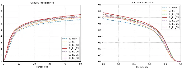
Precision plot evaluates the tracker’s ability to locate the target object by location error threshold, which is calculated by error between predicted bounding box with ground truth. In the diagram, the x-axis indicates the distance error (px) from 0 to 50, while the precision value that is corresponding to x shows the ratio of results within x px by all results.

Success plot evaluates tracker by the overlap ratio throughout test dataset. The overlap ratio is defined as the ratio of intersection by the overall area between bounding box with ground truth. In the success plot diagram, the x-axis indicates the overlap ratio from 0 to 1, while the success rate value corresponding to x shows the ratio of results larger than x by all results. 6.2 Results

6.2.1 Qualitative Self comparation. At first, we set the reward condition as: when predicted bounding box has the overlap ratio with ground truth which is larger than 0.7, the agent get +1 reward, otherwise the agent is penalized by getting -1 reward. However, the precision plot and accuracy plot don’t perform well. By analyzing some of result videos, we find that tracker

(37)

Figure 6.1. Testing results using RL training without distance error reward setting. In the Figure 6.1., the red bounding boxes denote the ground truth, while the green bounding boxes denotes the proposed bounding boxes from the tracker. The proposed bounding boxes are the results of our model, which is trained by RL without distance limitation reward setting.

During the analysis of these videos, some of them show up the above situations that the predicting bounding boxes are shrinking or enlarging through the video frame, which leads to low success ratio or even tracking failure.

Therefore, we believe the reward condition setting is not sufficient. Since the protocol of One Path Evaluation (OPE) has two criteria: location error and overlap ratio. Besides, the OTB evaluates trackers’ precision accuracy as their accuracy on 20px. Hence, we decided to modify reward function with location error conditions in six different thresholds as following setting:

𝑟𝑒𝑤𝑎𝑟𝑑(𝑠𝑇) = {

(38)

where 𝑑_𝑡ℎ𝑟 is chosen from the value list 𝑙𝑖𝑠𝑡_𝑡ℎ𝑟 = [10,15,20,25,30], which denotes the

distance (px) between predicted bounding box with ground truth. By changing the thresholds and train the model by RL differently, we get the comparation on different conditions of precision plot and success plot of OPE:

Figure 6.2. Qualitative self comparation respect to different distance limitation settings. In Figure 6.2., the read solid curve denotes the result when setting the threshold to 15px, and all the curves have labels of “SL_RL_x” denote the results in threshold setting at x px.

Based on results’ plots, we can tell that the accuracy of tracker is not positive

proportional to the threshold setting of the location error but reach the maximum accuracy at around 15-20px which happens to be the evaluation setting of OTB. Then we realize that testing videos have different velocity of object movement. Setting the location error threshold too high or too low can cause the tracker to choose poorly action series when the movement of the target object is too low or too high. Therefore, we aim to train adaptive policy by setting the location error condition part of reward condition according to the average location change during the RL training. The modified reward function is defined as following:

𝑟𝑒𝑤𝑎𝑟𝑑(𝑠𝑇) = {

(39)

which is the same as mentioned previous section, and the 𝑑_𝑠_𝑇_𝑎𝑣𝑒 denotes the average

distance change of target object in previous five frames.

Some of the results comparation with applying adaptive modification of reward function with the method training only using overlap ratio condition is:

Figure 6.3. Qualitative self comparation of adaptive reward setting with others. The comparation chart shows that the adaptive modification of reward function (curve with label “SL_RL_ad”) does improve the accuracy than the fixed threshold setting RL training

method and SL only training method.

(40)

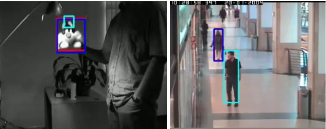
Figure 6.5. Comparison in individual sequences of adaptive reward setting and other. In Figure 6.4. and Figure 6.5. the red bounding box denotes the ground truth, the blue bounding box denotes the tracking result proposed by adaptive reward setting, and the cyan bounding box denotes the tracking result proposed by no adaptive reward setting.

6.2.2 Quantitative Comparation with other trackers. In order to compare with other trackers, we choose five different trackers’ test on individual sequences. The Tracking-Learning-Detection (TLD) tracker [25] doesn’t utilize CNN but has the same tracking strategy as ours during tracking process, while other four trackers are based on CNN structure. Deep

(41)

Table. 6.1. Quantitative comparation of proposed model with other trackers on IoU.

In Table. 6.1., the red mark denotes the best result in individual sequence, and the blue mark denotes the second-best result in individual sequence. Our proposed network performs well in “Dudek”, “BlurCar1”, and “Woman” sequences than others and has the highest average

overlap ratio than other trackers in these 22 sequences from OTB-100 dataset.

Ours DRLT TLD DLT CF2 HDT

Suv 0.730 0.621 0.660 0.743 0.822 0.823

Couple 0.551 0.493 0.761 0.237 0.594 0.586

Dudek 0.844 0.603 0.643 0.778 0.739 0.742

Human3 0.397 0.401 0.007 0.007 0.034 0.228

Human9 0.354 0.425 0.159 0.165 0.399 0.400

Jumping 0.690 0.651 0.662 0.598 0.717 0.738

Woman 0.766 0.479 0.129 0.595 0.726 0.744

Dancer 0.700 0.685 0.394 0.571 0.659 0.651

Liquor 0.590 0.532 0.456 0.342 0.723 0.643

BlurCar4 0.820 0.701 0.630 0.657 0.836 0.838

Human7 0.403 0.612 0.675 0.366 0.487 0.489

BlurCar2 0.868 0.693 0.726 0.732 0.765 0.770

Skater2 0.628 0.643 0.263 0.215 0.629 0.631

Bird2 0.692 0.473 0.570 0.221 0.847 0.835

Girl2 0.138 0.361 0.070 0.058 0.081 0.074

CarDark 0.502 0.548 0.423 0.582 0.647 0.664

CarScale 0.724 0.453 0.434 0.539 0.421 0.418

Car2 0.783 0.480 0.660 0.909 0.681 0.682

BlurCar3 0.759 0.680 0.639 0.205 0.811 0.765

BlurCar1 0.806 0.694 0.605 0.044 0.802 0.783

BlurBody 0.690 0.672 0.391 0.145 0.730 0.736

Dancer2 0.731 0.825 0.651 0.482 0.788 0.787

(42)

CHAPTER 7 Conclusion and Future Work 7.1 Conclusion

During my research, the results of some existing trackers tend to shrink the bounding boxes when the target object is partially occlusion, or there are distractors in the current frame. The proposed model aims to improve this type of video by adding an adaptive limitation of distance error to reward function during RL training.

Comparing to other trackers, which also utilize RL training and DNN features, our proposed model outperforms their behaviors in some sequences from the OTB-100 dataset like “Woman” and “Walking2”, where the target objects are partially occlusion by car or distracted

by the similar object during tracking.

Therefore, adding the limitation of distance to the condition of the reward function, and applying adaptive policy based on average distance change in previous frames does improve the performance in videos of OCC challenges. Besides, the adaptive policy setting model is better than no limitation setting model in OPE testing.

In short, different from tracking-by-detection based algorithms, our proposed model utilizes the sequential information by applying adaptive policy-based RL training and

outperforms some RL-based and CNN-based trackers in individual sequences from the OTB-100 datasets.

7.2 Future Works

(43)

tracking algorithms to enable models to track by utilizing higher-level features such as sequential information among video frames.

In this thesis, we improve the performance in scenarios that target is partially occluded, or the tracking algorithm is distracted by similar objects, by applying adaptive policy-based RL training. The adaptive policy-based RL means that on each frame during the training, this model is trained adaptively based on the average distance error in the previous five frames (sequential information). Therefore, our proposed model can handle object occlusion situation better than other RL based trackers and is more robust than other CNN-based trackers on videos that distractors appear during the tracking process.

However, there are still improvement opportunities in some challenges of object tracking task. One possible direction is reducing the influence of high variance. If the reward response from the mimic tracking environment during training by RL is always positive, the model might face the high variance problem. To handle this situation, the “baseline” trick in the policy

gradient algorithm is a possible improvement direction. Another difficulty for RL to handle is the comprehensive features. When tracking objects in videos like “Trans”, where maintaining

tracking object needs comprehensive features since the appearance of object changes rapidly in three seconds. It is possible that training another neural network using RL to extract

(44)

REFERENCES

1. Richard Szeliski, Computer Vision: Algorithms and Applications 2. Richard S. Sutton et al., Reinforcement Learning: An Introduction

3. Arnold W.M. Smeulders et al, Visual Tracking: An Experimental Survey, July 2014. 4. Yu Xiang et al., Learning to Track: Online Multi-Object Tracking by Decision Making,

February 2016

5. Sangdoo Yun et al., Action-Decision Networks for Visual Tracking with Deep Reinforcement Learning, November 2017

6. Pol Rosello et al., Multi-Agent Reinforcement Learning for Multi-Object Tracking, July 2018

7. Ken Chatfield et al., Return of the Devil in the Details: Delving Deep into Convolutional Nets, November 2014

8. Sarang Khim et al., Adaptive Visual Tracking Using the Prioritized Q-learning Algorithm: MDP-Based Parameter Learning Approach, September 2014

9. Janghoon Choi et al., Real-time Visual Tracking by Deep Reinforced Decision Making, June 2018

10. Ronald J. Williams, Simple Statistical Gradient-following algorithms for connectionist reinforcement learning, May 1992

11. Nicolai Wojke et al., Simple Online and Realtime Tracking with a Deep Associate Metric, March 2017

12. Daniel Gordon et al., Re3: Real-Time Recurrent Regression Networks for Visual Tracking of Generic Objects, December 2017

(45)

14. Da Zhang et al., Deep Reinforcement Learning for Visual Object Tracking in Videos, April 2017

15. Ming-xin Jiang et al., Multiobject Tracking in Videos Based on LSTM and Deep Reinforcement Learning, September 2017.

16. Boris Babenko et al., Visual Tracking with Online Multiple Instance Learning, June 2009 17. Samira Ebrahimi Kahou et al., RATM: Recurrent Attentive Tracking Model, April 2016 18. Luca Bertinetto et al., Fully-Convolutional Siamese Networks for Object Tracking,

September 2016

19. Yann LeCun et al., Gradient-Based Learning Applied to Document Recognition, November 1998

20. Visual Tracker Benchmark, from http://cvlab.hanyang.ac.kr/tracker_benchmark/ 21. Visual Object Tracking Challenge, from http://www.votchallenge.net/

22. https://medicalxpress.com/news/2018-07-neuron-axons-spindly-theyre-optimizing.html 23. PyTorch Community, https://pytorch.org/

24. Hyeonseob Nam et al., Learning Multi-Domain Convolutional Neural Networks for Visual Tracking, January 2016

25. Zdenek Kalal et al., Tracking-Learning-Detection, January 2010

26. Sam Hare et al., Struck: Structured Output Tracking with Kernels, 2015 27. Yi Wu et al., Object Tracking Benchmark, September 2015

28. Tom M. Mitchell, The Discipline of Machine Learning, July 2016

29. Naiyan Wang et al., Learning a Deep Comact Image Representation for Visual Tracking, December 2013

(46)

31. Yuankai Qi et al., Hedged Deep Tracking, December 2016

32. Liangliang Ren et al., Deep Reinforcement Learning with Iterative Shift for Visual Tracking, September 2018.

33. Martin Danelljan et al., Accurate Scale Estimation for Robust Visual Tracking, December 2016

34. Mohammad Ashraf, Reinforcement Learning Demystified: Markov Decision Processes, April 2018, from https://towardsdatascience.com/reinforcement-learning-demystified-markov-decision-processes-part-1-bf00dda41690

35. Ankit Choudhary, A Hands-On Introduction to Deep Q-Learning using OpenAI Gym in Python, April 2018, from https://www.analyticsvidhya.com/blog/2019/04/introduction-deep-q-learning-python

36. Soham Chatterjee, Different Kinds of Convolutional Filters, December 2017, from https://insuranalytics.ai/general/different-kinds-convolutional-filters/

37. Philip Ossenkopp, Reinforcement learning – Part 2: Getting started with Deep Q-Networks, December 2018, from https://www.novatec-gmbh.de/en/blog/deep-q-networks/

38. Sergey Levine, Policy Gradients, September 2017, from

http://rail.eecs.berkeley.edu/deeprlcourse-fa17/f17docs/lecture_4_policy_gradient.pdf 39. Pawan Jain, Complete Guide of Activation Functions, June 2019, from