Analytic Models for Acoustic Wave Propagation in Air

ABSTRACT

VETRENO, JOANNA RUTH. Analytic Models for Acoustic Wave Propagation in Air. (Under the direction of Dr. Michael B. Steer).

Ultrasound waves have been used for imaging purposes for many years. However, a liquid interface has always been necessary between the transducer and the object being imaged due to a high mechanical resistance at the air-transducer interface. Recent advances in transducers have made it possible to omit the liquid interface, allowing imaging to be done through air interfaces. Because this is a relatively new field, research into ultrasound propagation in air is very limited. A comprehensive model of how an ultrasound wave propagates through air would expedite the study of air-coupled ultrasound for imaging. This thesis presents a mathematical model of two-dimensional linear acoustic wave propagation in air. The model takes as input the frequency and amplitude of an acoustic signal and outputs the pressure field over varying longitudinal and lateral distances from the source. The benefits of a mathematical model over a finite element model are first

Analytic Models for Acoustic

Wave Propagation in Air

By

JoAnna R. Vetreno

A thesis submitted to the Graduate Faculty of North Carolina State University

in partial fulfillment of the requirements for the Degree of

Master of Science

Electrical Engineering

Raleigh, NC 2007 Approved by:

____________________________ ___________________________ Professor Michael B. Steer Professor Hamid Krim Chair of Advisory Committee

DEDICATION

To

Mike Adelson Omar Elshahawi

Yale Goodman Tim Kaefer Joseph Thurakal There from the beginning

Sue Hoyt & Carmen Kampf

BIOGRAPHY

JoAnna Vetreno was born on the 12th of August, 1983 along with a twin brother Michael. She grew up in Oakland, a small town in northern New Jersey. She received her Bachelor of Science (B.S.) degree in Electrical and Computer Engineering from Lafayette College, located in Easton, Pennsylvania, in 2006. In the fall of 2006 she began her graduate studies in the Electrical and Computer Engineering Department at North Carolina State University in Raleigh, NC, focusing on analog circuit design. She is a member of the Institute of Electrical and Electronics Engineers (IEEE), Eta Kappa Nu (HKN), the

TABLE OF CONTENTS

List of Tables ...vi

List of Figures ...vii

List of Symbols ...viii

1. Introduction ...1

1.1 Motivation ...1

1.2 Contribution ...3

1.3 Thesis Organization ...5

2. Physical Background ...6

2.1 Introduction ...6

2.2 Fundamentals of Acoustic Propagation ...6

2.3 Basic Oscillatory Motion ...8

2.3.1 Ideal oscillation ...8

2.3.2 Damped oscillation ...11

2.4 Basic Wave Motion ...13

2.4.1 The one-dimensional wave equation ...13

2.4.2 Forced vibration ...15

2.5 The Linear Acoustic Wave Equation ...16

2.5.1 Ideal linear wave equation ...16

2.5.2 Lossy wave equation ...18

2.6 Characteristic Properties of Plane Waves ...22

2.6.1 Decibel scales ...24

2.7 The Nonlinear Wave Equation ...25

2.7.1 Nonlinear oscillation ...25

2.7.2 The Westervelt equation ...27

2.8 Summary ...29

3. Modeling of the Acoustic Signal ...31

3.1 Introduction ...31

3.2 Investigations ...31

3.2.1 Study benefits and limitations ...32

3.3 Thesis Evolution ...33

3.3.1 Nonlinear 3D computer model ...34

3.3.2 Nonlinear 2D computer model ...35

3.3.3 Linear propagation model ...38

3.4 Summary ...39

4. Simulation Models ...41

4.1 Introduction ...41

4.3 Development of the Models ...42

4.3.1 Anechoic chamber ...42

4.3.2 Computer model ...45

4.4 Verification of the models ...49

4.4.1 Expected results ...50

4.4.2 Anechoic chamber verification ...52

4.4.3 Computer model verification ...55

4.5 Summary ...57

5. Mathematical Models of Acoustic Propagation ...59

5.1 Introduction ...59

5.2 Lateral propagation characteristic ...59

5.2.1 Anechoic chamber ...59

5.2.2 Computer model ...61

5.3 Mathematical model ...67

5.3.1 Polynomial fit ...67

5.3.2 Hermite-Gaussian fit ...70

5.4 Summary ...76

6. Conclusions ...77

6.1 Conclusions ...77

6.2 Future Work ...78

Appendix ...79

Appendix A COMSOL model report ...80

Appendix B Raw chamber data ...95

LIST OF TABLES

LIST OF FIGURES

Figure 1.1 Medical sonography of the carotid artery and underwater sonic imaging ...2

Figure 1.2 Mathematical model block diagram ...4

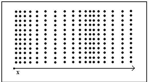
Figure 2.1 Compression and rarefaction of air particles due to longitudinal wave propagation through a medium ...8

Figure 2.2 Diagram of a mass on a spring ...9

Figure 2.3 Particle displacement, speed, and acceleration ...11

Figure 2.4 Diagram of a mass on a spring with viscous damping ...12

Figure 2.5 Propagation of a transverse disturbance along a taut string ...13

Figure 2.6 Absorption coefficient of sound in air at 20 °C and 1 atm (101,325 Pa) for various relative humidities ...22

Figure 3.1 Various mesh shapes for finite element modeling ...37

Figure 4.1 The makeup of the acoustical blocking material on the anechoic chamber walls, floor, and ceiling ...43

Figure 4.2 E&M tile used for the outermost layer in the chamber absorption tiles ...44

Figure 4.3 Schematic of anechoic chamber setup for longitudinal wave propagation experiment ...45

Figure 4.4 COMSOL computer model of the Anechoic Chamber ...48

Figure 4.5 Expected exponential peak decay for the measured results ...51

Figure 4.6 Expected peak decay for the computer model results ...52

Figure 4.7a Raw data packet collected from measurements in the anechoic chamber ...53

Figure 4.7b Measured longitudinal peak decay ...54

Figure 4.8 COMSOL computer model longitudinal peak decay ...56

Figure 5.1 Measured lateral propagation characteristic ...60

Figure 5.2 Transient 2D COMSOL computer model results ...62

Figure 5.3 COMSOL computer model constant phase arcs ...63

Figure 5.4 COMSOL computer model lateral propagation characteristic ...64

Figure 5.5 COMSOL computer model lateral propagation characteristic at 50k Hz ...66

Figure 5.6 Polynomial curve fit to the lateral propagation characteristic ...68

Figure 5.7a 12th order Hermite-Gaussian function ...70

Figure 5.7b 12th order Hermite Polynomial ...70

Figure 5.8 Equation (5-4) fit to the lateral propagation characteristic ...72

Figure 5.9 Hermite-Gaussian curve fit to the lateral propagation characteristic ...74

LIST OF SYMBOLS

Symbol Unit Description

a unit less Linear scaling factor

) , (x t

av m/s2 Particle acceleration

A m Oscillation amplitude

b unit less Nonlinear restoring force

B Pa Adiabatic bulk modulus

A

B/ unit less parameter of nonlinearity

c m/s Speed of wave propagation

o

c m/s Speed of sound propagation

℘

c J/(kg*K) Specific heat at constant pressure

CFL unit less Wave distance per time step

o

f Hz Source frequency

y

f N Force element in the ydirection

F N Force

r

F N Viscous friction force

h m Maximum mesh element size

I W/m2 Intensity

ref

I W/m2 Reference intensity

) (t

I W/m2 Instantaneous intensity

IL dB Intensity level

k rad/m Wave number

l m Length of source

L unit less Second-order Lagrangian

m kg Mass

o

M unit less Amplitude mach number

N unit less Resolution parameter

'

p Pa Perturbation pressure

o

p Pa Equilibrium pressure

o

P Pa Initial pressure amplitude

REF

P Pa Reference pressure

RMS

P Pa Root mean square pressure

) , (x t

p Pa Acoustic pressure

Psq Pa2 Square of instantaneous pressure

R m Distance from source

m

Symbol Unit Description

s N/m Spring constant

c

s unit less Condensation

SPL dB Sound pressure level

t s Time

MAX

t s Limiting time step size

T s Period of a wave

s

T N Tension

o

u m/s Initial velocity

) , (x t

uv m/s Particle velocity

d

x m Discontinuity distance

o

x m Initial displacement

) , (x t x v

m Particle displacement

o

Z Pa*s/m Specific acoustic impedance

α Np/m Attenuation coefficient

α dB/m Attenuation coefficient in decibels

d

α Np/m Damping coefficient

κ

α Np/m Thermal attenuation

v

α Np/m Viscous attenuation

β unit less Coefficient of nonlinearity

γ unit less Ratio of specific heats

δ m2/s Diffusivity of sound

η Pa*s Shear viscosity coefficient

B

η Pa*s Coefficient of bulk viscosity

κ W/(m*K) Thermal conductivity

λ m Wavelength

ρ kg/m3 Instantaneous density

L

ρ kg/m Linear density

o

ρ kg/m3 Equilibrium density

'

ρ kg/m3 Perturbation density

τ s Retarded time

φ rad Phase

Ψ m2/s Velocity potential

d

ω rad/s Damped natural frequency

o

Chapter 1 Introduction

1.1

Motivation

Using high frequency acoustics (ultrasound) for imaging, non-destructive testing, and other purposes is a common and well understood practice. However, to date all methods of using ultrasound for imaging have relied on a fluid coupling between the transducer and the media being tested or imaged. There is increasing interest in the use of noncontact, gas coupled ultrasound in imaging for many reasons. It is simpler, lower in cost, and, by removing the usual fluid coupling requirement, allows imaging of objects a distance away and in applications where a liquid coupler is impractical.

Figure 1.1: Medical sonography of the carotid artery (left [1]) and underwater sonic imaging (right [2])

Using ultrasound for imaging in biomedical and underwater applications is a fairly well understood and well researched phenomenon. However, it relies on a transducer-liquid-media interfacing for its functionality. Of great interest lately is the possibility of using ultrasound for imaging without the need of the liquid interface between the transducer and the media being tested. Previously, this field had been limited by the high mechanical impedance mismatch of a transducer-air interface, causing low coupling and high loss of the acoustic wave into the air. However, recent advances in the generation of transducers have made this problem less significant, opening the door to ultrasound testing with transducer-air-object interfacing.

the studies focusing on the various transducer varieties, how to design them for good air coupling, and how properties of air affect acoustic propagation.

An immense body of research exists on the characterization of ultrasound activity in liquid and solid media, but there is surprisingly little on the propagation of ultrasound in gases, given the possibilities for the field. Currently, the majority of work has been

examinations of how the atmosphere decays the acoustic wave and studies of the design and characterization of the transducers that generate the ultrasound. What is lacking in the research of air coupled ultrasound is a fast computation model that can predict the propagation field in air. Such a model would make it easier to predict ultrasound interactions with and reflections from objects based on initial pressure level and propagation distance information.

1.2

Contribution

supported by the computers in existence today. This requirement severely limits the size of the model that can be created and greatly increases computation time, to a point where the model is no longer useful.

It is therefore useful to come up with a mathematical model of the wave propagation, which can significantly reduce computation time when studying wave interaction with objects and air. The goal of such a model (Figure 1-2) is to predict the spread and propagation of an ultrasound wave given only its initial amplitude and frequency.

Figure 1.2: Block diagram of the mathematical model for predicting the two dimensional propagation characteristic of ultrasound in the atmosphere. Given an initial amplitude and frequency, the model computes the 2D wave field.

1.3

Thesis Organization

Chapter 2 gives a detailed review of the basic physical phenomena and equations that govern acoustic propagation, both linear and nonlinear. Chapter 3 examines

pre-existing research in the field and then outlines the development of this thesis topic. Chapter 4 presents an experimental model and a computer model and verifies the accuracy of those models. Results from these models will be used to generate the mathematical model. Chapter 5 presents experimental data from the models and then details the development of the mathematical model for acoustic propagation in the atmosphere. Chapter 6 concludes the work done and gives some guidelines for future work.

REFERENCES

[1] Image taken from the National Heart Lung and Blood Institute, Diseases and Conditions Index website on November 20th, 2007.

http://www.nhlbi.nih.gov/health/dci/Diseases/cu/cu_all.html

[2] Image taken from the Khuri-Yakub Ultrasonics Group website on November 20th, 2007.

Chapter 2 Physical Background

2.1

Introduction

When ultrasound is used for imaging, one or two directional tones are transmitted via a transducer into the air, after which reflections of the sound beams are recorded and used to determine various properties of the object under examination. Therefore, of interest in this research is the propagation of single tone directed ultrasound. This chapter presents a detailed background on acoustic propagation but focuses on the propagation of single tone plane waves. Before delving into the topic of ultrasonic acoustic propagation, it is

beneficial to review the basics of particle oscillation that lead to the transmission of acoustic waves through a medium. This chapter gives a general review of the physical equations that govern both linear and nonlinear wave motion through the air, and presents the partial differential equation that describes the pressure variation of a medium as a single frequency acoustic wave propagates. If the reader already has a strong background in wave motion then they are encouraged to jump ahead to the derivation of the damped linear wave equation (Section 2.5.2) and the nonlinear Westervelt equation (Section 2.7) which are the most pertinent equations for this thesis.

2.2

Fundamentals of Acoustic Propagation

molecules back. This elastic force, along with inertia, causes the molecules to oscillate, allowing acoustic waves to propagate. The oscillatory motion is analogous to the motion of a spring when displaced from its rest position, while the propagation of the wave itself is analogous to the movement of a wave down a piece of string. The most well known

acoustic waves are those of sound. The audible frequency range for an average person is 20 Hz to 20k Hz; the range above the audible (greater than 20k Hz) is called the ultrasonic region, and the range below the audible (less than 20 Hz) is called the infrasonic region.

This thesis will concern itself only with acoustic waves in air, and the assumption is made that the waves are plane waves. To be planar means that each acoustic variable has constant amplitude on any given plane perpendicular to the direction of propagation. This assumption greatly simplifies the derivations of acoustic equations and relationships, and is valid in most experimental situations because wave fronts of any divergent wave in a

homogeneous medium become approximately planar when sufficiently far from the source. Sufficiently far from the source means that the wave is in the far field, as opposed to the near field. The separation distance that designates far from near is given by

λ 2

l

R >> (Equation 2-1)

where l is the length of the source, λ is the wavelength of the wave and R is the measuring distance from the source [1].

(Figure 2.1). This produces adjacent regions of compression and rarefaction of the air particles as the wave moves.

Figure 2.1: Compression and rarefaction of air particles due to longitudinal wave propagation through a medium.

Speaking of wave propagation in terms of air particles is more accurate that air molecules, because in general molecules move through a medium in erratic and unpredictable manners. Instead, a particle of the medium is defined which is small enough to assume that all

physical quantities are constant across the particle but large enough to assume that the random motion of the molecules within the particle average out to uniform.

2.3

Basic Oscillatory Motion

2.3.1 Ideal oscillation

Figure 2.2: Diagram of a mass on a spring [2]

The mass is analogous to a single air particle and the spring is analogous to the previously described restoring elastic forces. When the mass m in kilograms (kg) is displaced in the positive x direction in meters (m), a restoring force F in newtons (N) can be defined by the equation

x s

F =− * (Equation 2-2) where s is the spring constant of the spring in N/m. Combining this with the general equation of motion

2 2 * dt x d m

F = (Equation 2-3)

where ₂ 2

dt x d

is the acceleration of the mass, yields the differential equation

0 2 2 = + x m s dt x d (Equation 2-4)

This differential equation has the general solution ) sin( )

cos( )

(t A₁ t A₂ t

where A₁ and A₂ are arbitrary constants defined by initial conditions and ω_o is the natural angular frequency, defined by s/m. The general solution can be transformed into a more useful solution by defining A₁ = Acos(φ)and A₂ =−Asin(φ) where A is the motion

amplitude and φ is the initial phase angle, which when substituted into Equation 2-5 gives the final solution

) cos(

)

(t = A ω t+φ

xv _o (Equation 2-6) Definitions of A and φ can be derived by examining the initial conditions of the system. If the spring at time t =0 has a position x_o with an initial speed u_o, then substitution and differentiation shows that

2 2

) / ( o o

o u

x

A= + ω (Equation 2-6a) ) ( tan 1 o o o x u ω φ = − − (Equation 2-6b)

Equations for velocity and acceleration of the particle can be obtained by successive differentiation of Equation 2-6:

) sin(

)

(t =−ω A ω t+φ

uv _{o o} (Equation 2-7) )

cos( )

(t =−ω2A ω t+φ

Figure 2.3: Particle displacement, speed, and acceleration of plane

wave propagation [2]

2.3.2 Damped oscillation

Any real physical system has dissipative forces that act against the motion of oscillation, which cause the amplitude of oscillation to reduce with time. The type of force that causes the dissipation varies depending on the type of oscillation being examined, but all result in the overall damping of the oscillations. For the mass on a spring example examined in the last section, a viscous friction force Fr can be used to demonstrate the

Figure 2.4: Diagram of a mass on a spring with viscous damping [2].

The force Fr is assumed to be proportional to the velocity of the mass

dt dx R

F_r =− _m (Equation 2-9)

where R_m is a constant representing the mechanical resistance of the system. When combined with Equation (2-4), the damped equation of oscillatory motion becomes

0 2 2 = + + sx dt dx R dt x d

m m (Equation 2-10)

The completed solution to this equation is

) cos(

) exp( )

(t = A −α t ω t+φ

x _{d d} (Equation 2-11) m

R_m

d = /2

α (Equation 2-11a) 2

2

d o

d ω α

ω = − (Equation 2-11b)

main effect of damping on oscillatory motion is an exponential decay on the amplitude of the particle motion.

2.4

Basic Wave Motion

2.4.1 The one-dimensional wave equation

The equation of motion for wave propagation can be described using the example of an ideal vibrating string. Many simplifying assumptions are made in this example in order to make the derivation easier, but the results are still very useful in developing a

fundamental understanding of wave motion. If a taut string is displaced from equilibrium and then released, the displacement, shown in Figure 2.5, is seen to break into two

displacements that propagate along the string in opposite directions.

Also, the speed that the displacement propagates at is seen to be independent from the amplitude of the initial disturbance and instead depends only on properties of media that the wave is propagating in. For a string, the speed of propagation is given by

c= T_s /ρ_L (Equation 2-12) where T_s is the tension in N and ρ_L is the linear density of the string in kg/m. The motion of a wave propagating down a string is called a transverse traveling wave, which means that the particle displacement caused by the disturbance is perpendicular to the direction of propagation.

The equation for wave propagation is developed by considering the forces that act on the string to bring it back to equilibrium. Given a plucked string of uniform linear density and negligible stiffness, stretched to a tension T_s which is large enough so that the forces of gravity acting on the string can be ignored, the net transverse force on a small element of the string can be described by

dx x

y T dfy s 2

2

∂ ∂

= (Equation 2-13)

Combining this with the general equation of motion for the system,

2 2

t y dx dfy L

∂ ∂

=ρ (Equation 2-14)

This differential equation has the general solution ) ( ) ( ) ,

(x t y₁ ct x y₂ ct x

y = − + + (Equation 2-16) In this solution, y₁(ct−x) represents the wave traveling in the positive x direction and

) ( 2 ct x

y − represents the wave that travels in the negative x direction. Possible functions for y include sin[ω_o(t±x/c)], log(ct±x), and exp[jω_o(t±x/c)], among many others.

2.4.2 Forced vibration

Most vibrations, whether they are mechanical, electrical, or acoustical, are driven by an externally applied force. In mechanics this can be a piston, in electronics a signal

generator, and in acoustics a vibrating membrane, or transducer. For a string, the simplest type of forced vibration is achieved by applying a transverse sinusoidal driving force to one end of an ideal string of infinite length.

Apply a driving force Acos(ω_ot) at position x=0 of an ideal string of infinite length and assume that the end of the string does not move in the x direction but is free to move in the y direction. Because the string is infinitely long, waves due to the driving force will propagate only in the positive x direction

) ( ) ,

(x t y₁ ct x

y = − (Equation 2-17) Using boundary conditions and the known driving force, y1 can be solved for as

) cos(

) ,

(x t A t kx

y = ωo − (Equation 2-18)

c k =ωo

(Equation 2-19)

Note that Equation (2-18) is very similar to the solution found for the differential equation of oscillatory motion, Equation (2-6). The difference here is that the phase, φ, is

determined by characteristics of the driving force and the media.

2.5

The Linear Acoustic Wave Equation

2.5.1 Ideal linear wave equation

As stated in Section 2.2, acoustic waves are caused by pressure fluctuations in a compressible fluid. To develop an equation for acoustic wave propagation, it is easiest to begin with the ideal case of propagation through an inviscid fluid. An inviscid fluid is a fluid in which the effects of friction due to viscosity can be ignored, meaning that the viscous effects are relatively small compared with the inertial restoring forces of the fluid [3]. It also means that losses due to attenuation through the media are ignored, making this a lossless equation for acoustic propagation. This equation is often a valid approximation because in many situations dissipation is so small that it can be ignored for the frequencies or distances of interest.

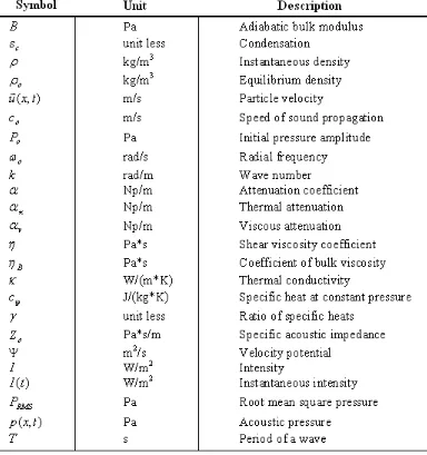
Before beginning, a few terms are defined in Table 2-1 which will aid in the

Table 2-1 Table of useful symbols

Using the governing physical equations for sound, the linear wave equation can be derived. These equations are the linear equation of state,

0 = ⋅ ∇ + ∂ ∂ u t o v ρ ρ (Equation 2-21)

and the linear equation of force, also known as Euler’s Equation

p t

u

o _∂ =−∇

∂v

ρ (Equation 2-22)

Combining Equations (2-20), (2-21), and (2-22) yields a single differential equation with one dependant variable

0 1 2 2 2 2 = ∂ ∂ − ∇ t p c p o (Equation 2-23)

This equation is the linear, lossless wave equation for the propagation of sound in fluids with phase speed c_o. Because this equation is very similar to Equation (2-15), the equation for one-dimensional wave propagation, the development of solutions already completed for Equation (2-15) can be applied here, yielding the solution

p(x,t)=P_ocos(ω_ot−kx) (Equation 2-24)

2.5.2 Lossy wave equation

added to the equation for viscous losses. It is easiest to derive the lossy wave equation due only to propagation through a viscous medium and then to include losses due to thermal conduction.

All real media have some viscosity associated with them. In air, the viscosity is very low and therefore losses are small. In addition, attenuation effects in air are directly proportional to the square of the operating frequency. Therefore, in acoustic studies where the bandwidth of interest is the audible bandwidth, the frequency is low causing the

attenuation to be as low as 10-5

Np/m. Across distances up to 1000 m, these attenuation effects are negligible and therefore attenuation due to viscous friction loss can generally be ignored, which is why the inviscid wave equation is most often used. However, attenuation increases as frequency increases, so for frequencies in the range of 30k Hz and above, the attenuation becomes as large as 10-1 Np/m. Even across distances as short as 1 m, the effect of this attenuation is noticeable and viscous effects must be taken into account.

To include dissipation in the form of viscosity, the governing physical equations for sound propagation must be reexamined. The equation of continuity is not changed by the presence of viscosity, and remains equivalent to Equation (2-21). The equation of state also remains the same despite the presence of viscosity because the viscous contribution to this equation is nonlinear and therefore falls out when the equation is linearized. Therefore, the equation of state remains equivalent to Equation (2-20). This leaves only Euler’s Equation to be changed by the inclusion of viscosity effects.

u u p t u o B v v v 2 2 1 4

3 _{) ( )}

( + ∇ ∇⋅ − ∇ = ∇ + ∂ ∂ _{η η ρ}

ρ (Equation 2-25)

where η is the shear viscosity coefficient and η_B is the coefficient of bulk viscosity. For a more detailed examination on the derivation of this equation and all the governing physical equations the reader is referred to Saad [4].

Combining Equations (2-20), (2-21) and (2-25) again yields a single differential equation with one dependant variable

0 1 2 2 2 2 2 = ∂ ∂ ∇ + ∂ ∂ − ∇ t p t p c p s o

τ (Equation 2-26a)

2 75 . o o B s c ρ η η

τ = + (Equation 2-26b)

This equation is the linear, dissipative wave equation for the propagation of sound in fluids. Note that it is identical to the lossless equation except for the added third term on the left hand side which can be considered the viscous dissipative term.

For a plane wave traveling in the +x direction, the solution to Equation (2-26a) is defined as ) cos( ) exp( ) ,

(x t P x t kx

p = _o −α ω_o − (Equation 2-27) where α is the attenuation coefficient in Np/m which causes the amplitude to decay in an exponential form.

2 2 / 1 2 ) ( 1 1 ] ) ( 1 [ 2 1 s o s o o o v

c ω τ

τ ω ω α + − +

= (Equation 2-28)

As mentioned above, attenuation due to thermal conduction is most easily found

heuristically from physical arguments. The derivation is not done here but can be found in Blackstock [5], the equation being

℘ − = c co o

o γ κ

ρ ω

α_κ ( 1)

2 3

2

(Equation 2-29)

where γ is the ratio of specific heats, κ is the thermal conductivity and c_℘ is the specific heat at constant pressure.

It can be shown that for small losses (which is the case for propagation through air, even at high frequencies), independent sources of acoustic loss can simply be summed together to create the total absorption coefficient

∑

= i

i

α

α (Equation 2-30a)

) ) 1 ( 75 (. 2 3 2 ℘ − + + = c

c_o B

o

o η η γ κ

ρ ω

α (Equation 2-30b)

Figure 2.6: Absorption coefficient in dB/(100 m*atm) of sound in air at 20 °C and 1atm (101,325 Pa) for various relative humidities [5].

2.6

Characteristic Properties of Plane Waves

Recall also that in general, most waves can be considered planar when sufficiently far from the source, as stated in Section 2.2. Therefore defining some special properties of plane waves becomes very useful.

The solution for the pressure field p(x,t) of a plane wave is described in Equation (2-24). From this, the velocity and velocity potential equations of a plane wave can easily be derived. Due to inherent properties of the plane wave already described, velocity of the wave differs from pressure by only a constant.

o oc t x p t x u ρ ) , ( ) , ( v v ₌ (Equation 2-31)

where ρ_oc_o is defined as the specific acoustic impedance Z_o of the media. This impedance is analogous to the wave impedance µ/ε of a dielectric medium for electromagnetic waves and to the characteristic impedance of a Z_o of a transmission line. The velocity potential equation is almost as easily obtained, being related to pressure by a complex constant o o j t x p t x ρ ω ) , ( ) , ( v v =

Ψ (Equation 2-32)

The linear relationship between pressure and velocity is very useful, especially when developing equations for acoustic intensity. The instantaneous intensity

) , ( * ) , ( )

(t p x t u x t

in W/m2

of an acoustic wave is the instantaneous rate per unit area at which work is done by one element of the fluid medium on an adjacent element. From this, the intensity I can be defined as the time average of I(t)

∫

1 v v

(Equation 2-34)

where T is the period of the wave. In acoustics and many other wave phenomena, the velocity of the wave particle is very hard to measure, but the pressure is a known quantity. Therefore, it is easiest to substitute Equation (2-27) into the equation for intensity, yielding

o o o c P I ρ 2 2 ±

= (Equation 2-35)

It must be stressed that the uv(t) substitution is only valid when dealing with plane waves or with diverging waves that are very far from the source. If this is not the case, the intensity calculation is much more complicated.

2.6.1 Decibel scales

Sound pressures and intensities are often described using log scales because their values can vary over such a wide range; audible intensities alone can range from 10-12

to 10 W/m2. Using log scales, one can define an intensity level IL of a sound intensity I by

) log( 10 REF I I

IL= (Equation 2-36)

where I_REF is a reference intensity that has a value of 10-12 W/m2

) log( 20

REF RMS

P P

SPL= (Equation 2-37)

where P_REF is a reference pressure that has a value of 20μ Pa for air and P_RMS is the root mean square pressure value, defined by

2

o RMS

P

P = (Equation 2-38)

Both SPL and ILhave units of decibels, or dB.

2.7

The Nonlinear Wave Equation

Previously, all of the equations that were derived for acoustic propagation assumed that the propagation through air was a linear phenomenon. While this assumption is valid when explaining most small signal, low frequency acoustical phenomena, the assumption no longer holds when examining ultrasonic propagation. Nonlinear effects of both the air and the vibrating particles make significant contributions to the propagation of a sound wave through air, usually in the form of wave distortion and higher order frequency generation.

2.7.1 Nonlinear oscillation

) cos( 2 2 t A sx t x

m + = ω_o

∂ ∂

(Equation 2-39)

where sx is the linear equation for the restoring force of the spring. However, if the linear restoring force is replaced with a nonlinear one,

3

bx sx

sx_NL = + (Equation 2-40) then Equation (2-39) can be solved for a first and a second order approximate solution. This nonlinear situation is similar to having springs of differing “stiffness”. If b>0, it equates to a stiffer or harder spring, and if b<0 it equates to a spring with a lower effective stiffness, or a softer spring. Solving this equation for the first and second order nonlinear approximations, one finds that the first order term is the same as the linear solution,

) cos(

) (

1 t =A ω t+φ

x _o (Equation 2-41) and the second order approximation after many calculations and simplifications is

) 3 cos( 32 ) cos( ) ( ₂ 3 1 2 t m bA t A t x _o o o ω ω ω +

= (Equation 2-42)

This is a very simplified example of what one small nonlinear contribution can do to change the solution of a system. The mathematics behind the derivations for these

equations was not duplicated here due to length, but can be found in Beyer [6]. The next step is to see how the inclusion of nonlinearities affects the linear acoustic wave equation.

2.7.2 The Westervelt equation

Deriving a nonlinear wave equation involves extensive mathematics and has been done in many forms and with many different contributing factors. The most complete equation that is also similar in form to the linear wave equations already derived is the Westervelt equation. This equation describes the propagation and diffraction of acoustic waves through a homogenous medium with attenuation and nonlinear behavior.

The nonlinear Westervelt equation is derived by returning again to the governing physical equations for sound propagation: the equation of state, the equation of continuity, and Euler’s equation. This time, however, the equations are not linearized into their simplest form but are instead given a second order approximation based on the original full equations.

To make a second order approximation of the equation of continuity, substitute '

ρ ρ

ρ = o + into the equation, where 'ρ is a slight deviation from equilibrium density.

This substitution yields

' '

' _{ρ ρ ρ}

ρ _{+ ∇⋅ =− ∇⋅ − ⋅∇}

∂ ∂

u u u

t o

v v v

in which the first order terms are on the left side of the equals sign and the second order terms are on the right side. For Euler’s Equation (the equation of momentum) p= p_o + p', where 'p is a slight deviation from equilibrium pressure, is substituted into the equation yielding t u u u p t u o B o _∂ ∂ − ∇ − ⋅ ∇ ∇ + = ∇ + ∂

∂v v v v

' )

( )

( ₂1 2

4

3η η ρ ρ

ρ (Equation 2-44)

Notice that it also contains the viscous parameters introduced in Equation (2-25). Again, the first order terms are on the left side of the equal sign and the second order terms are on the right side. The equation of state is turned into a second order approximation by

expanding it in a Taylor series about the equilibrium state (ρ_o,s_o) and ignoring third order terms 0 , 2 2 2 ) ( ' ' 2 ' ρ _ρ ρ ρ s p s A B c c p o o o ∂ ∂ + +

= (Equation 2-45)

where B/A is the parameter of nonlinearity. There are many different equations for B/A depending on the medium and what parameters are being varied. However, for ideal gases,

A

B/ can be replaced by (γ −1)[7]. Air, being composed mostly of nitrogen, can be approximated as an ideal gas giving it a B/A of 0.4.

Various manipulations of Equations (2-43), (2-44) and (2-45) and the subsequent combinations of those equations leads to a full nonlinearity equation

where β =1+B2A is the coefficient of nonlinearity, δ is the diffusivity of sound, and L is

the second-order Lagrangian density

2 2 2

2 1

2 _{o o}

o c p u L ρ ρ −

= v (Equation 2-47)

The Westervelt equation is obtained from this by discarding the term containing L, which is valid for plane waves because at first order, p= ρ_oc_ouv. The Westervelt equation then becomes 2 2 2 4 3 3 4 2 2 2 2 1 t p c t p c t p c p o o o o ∂ ∂ − ∂ ∂ − = ∂ ∂ − ∇ ρ β δ (Equation 2-48)

in which the first order terms are on the left side of the equal sign and the second order terms are on the right side. As mentioned before, there are many other forms of the

nonlinear wave equation. However, the Westervelt equation has been found to be the most accurate for monotone directed plane progressive sound beams [8], which is what this thesis concerns itself with.

2.8

Summary

This chapter gave detailed background information on how acoustic wave

REFERENCES

[1] Möser, Michael, Engineering Acoustics: An introduction to noise control, New York, New York: Springer, 2004.

[2] Kinsler, Lawrence E., Fundamentals of Acoustics, New York, New York: Wiley Inc., 2000.

[3] Munson, Bruce, Young, Donald, and Okiishi, Theodore, Fundamentals of Fluid Mechanics, 4th Ed.New York, New York: Wiley Inc., 2002.

[4] Saad, Michel A., Compressible Fluid Flow, Second Edition, New Jersey: Prentice-Hall, Inc., 1993.

[5] Blackstock, David T, Fundamentals of Physical Acoustics, New York: Wiley Inc., 2000.

[6] Beyer, Robert T., Nonlinear Acoustics, New York, New York: Acoustical Society of America, 1997.

[7] Hamilton, Mark F. and Blackstock, David T. “On the coefficient of nonlinearity β in nonlinear acoustics,” Journal of the Acoustical Society of America, vol. 83, no. 1, pp.74-77, January 1988.

Chapter 3 Modeling of the Acoustic Signal

3.1

Introduction

Using ultrasonic interaction and reflections from an object for imaging without the use of a liquid interface between the transducer and the object being observed is a relatively new endeavor. Therefore, the research into ultrasound propagation through air is still in the first stages, looking mainly at the behavior of the transducers being used to generate the sound and the effects of air on ultrasound propagation. The majority of research that exists on ultrasound imaging in general involves propagation in water (mostly oceanic) or in biological medium because ultrasonic coupling into a liquid is much higher than it is for air and has therefore been in use longer. Because ultrasonic propagation in air is such a new field, the capabilities and deficiencies of various modeling tools are as yet unknown. This chapter first investigates some of the existing work on ultrasonic propagation in air and then details the development of this thesis, which went through many stages due to the

restrictions of modeling tools.

3.2

Investigations

interest due to a large mechanical mismatch at the transducer/air interface. However, with recent developments in ultrasonic transducers, mainly in the reduction of the influence of the mechanical mismatch, it has become more feasible to use an air interface for imaging purposes.

With these advancements in ultrasound transducers have come some limited studies into ultrasound propagation in air. These studies generally examine the propagation characteristics of ultrasonic propagation but few attempt to derive fast computation models of the propagation, which would be beneficial in furthering the study of using air coupled ultrasound for imaging.

3.2.1 Study benefits and limitations

by the transducers, including 2D spread characteristics very similar in appearance to the lateral spread characteristic examined and modeled by this thesis.

What all of the previous research lacks is the generation of a fast computational method that models linear and nonlinear, longitudinal and lateral ultrasound propagation in air. One such study that is being done in this field is by Garner [4]. It furthers work done by Stoessel [5] by creating a one dimensional model that generates a single tone

propagating in air. The nonlinearities inherent in air cause energy from the single tone to spread into second and third order harmonics. The effect is modeled using both a Bessel approximation and a Perturbation approximation, and is accurate to the discontinuity distance [5]

o d

M k x

β 1

= (Equation 3-1)

where Mo is the amplitude Mach number. This model does not take into account

attenuation as the wave propagates, and is only valid for longitudinal propagation.

3.3

Thesis Evolution

their conclusions. Below is a list of the development steps, followed by a description of how one topic led to another, ending in the final thesis that this paper discusses.

• Nonlinear 3D computer model of ultrasonic acoustic wave propagation and interaction at the boundary between media.

• Nonlinear 2D computer model of ultrasonic acoustic wave propagation and interaction at the boundary between media.

• Linear 2D computer model of ultrasonic acoustic wave propagation.

• Linear mathematical model of the lateral pressure spread of an ultrasonic acoustic wave.

As discussed in Chapter 1, this thesis is part of an ongoing study into how

ultrasound waves can be used to create images of and characterize items at a distance from the observer or buried under the ground.

3.3.1 Nonlinear 3D computer model

applications where the wavelength is on the order of a millimeter, a 3D model is no longer practical (the simulation field could be no larger than a few tens of millimeters cubed). This limitation led to the revision of using a 2D model for acoustic propagation.

3.3.2 Nonlinear 2D computer model

Upon switching to a 2D model, it was found that simulations of a reasonable size (50*λ rather than 5) could be completed in about an hour or two of real time for a few milliseconds of simulated time. This long simulation time sent up a red flag, pointing to the need for creating a mathematical model that would run much faster. The general idea at this point was to create the nonlinear computer model and use that along with experimental data to generate a mathematical model that would be able to compute solutions much faster than the computer model.

COMSOL Multiphysics defaults to a linear model for acoustic propagation but has a weak equation system that can be used to include nonlinearities in the model. The most common examples that COMSOL gives for incorporating nonlinearities into a model is through a nonlinear material or property. However, for acoustic wave propagation, the nonlinearities appear in the differential equation that the computer model implements to solve for the pressure of the radiating acoustic field. To incorporate this, the test function had to be used, which is a function that enables the generation of higher order derivatives and the mixing of space and time derivatives.

equation in existence, and each one has its own benefits and pitfalls. The first equation that was considered was the KZK equation,

0 2 2 2 3 3 3 2 2 2 3 2 = ∆ − ∂ ∂ − ∂ ∂ − ∂ ∂ ∂ p c p c p c z p o o o o τ δ τ ρ β

τ (Equation 3-1)

which has been widely used to model the paraxial region of a nonlinear sound beam. In this equation, τ is the retarded time. This equation is based on a parabolic approximation, and is considered valid for directional sound beams. However, the KZK equation becomes less valid for distances close to the source and for angles 20° or more off the axis of the

transducer [7]. Because this thesis examines the acoustic field at varying distances from the source and for many lateral distances, an equation that is accurate over a larger spread was desired. According to Huijssen [8], the Westervelt equation,

0 1 2 2 2 4 3 3 4 2 2 2 2 ₌ ∂ ∂ + ∂ ∂ + ∂ ∂ − ∇ t p c t p c t p c p o o o o ρ β δ (Equation 3-2)

which is a full nonlinear wave equation, is a much more comprehensive equation that accurately depicts the acoustic field both near and far from the source and at higher degrees from the beam axis. In fact, the KZK equation can be considered an approximation of the Westervelt equation. An explanation and derivation of the Westervelt equation can be found in Section 2.7.2.

equation, the shape used to create the element mesh of the model should have 8 nodes (see Figure 3.1) for best resolution of the nonlinear effects. The default mesh size in COMSOL is a 3 node triangle mesh, and the highest mesh that can be utilized is a 4 node mesh. This limitation raised some initial concerns with COMSOL’s ability to accurately model the nonlinear equation.

Figure 3.1: Various mesh shapes for finite element modeling. Computations are performed at the nodes, where different elements meet. Higher order

computations require higher noded mesh elements.

The model was meshed using the four node shape.

Weak term: −px*test(px)− py*test(py) (Equation 3-3a)

Time-dependant weak term: * ₂ ( )

o c p test ptt (Equation 3-3b)

where px, ptt, etc. are the first and second derivatives of pressure with respect to x and t, respectively. Converting the Westervelt equation using the test function yields an equation of

Weak term: −px*test(px)− py*test(py) (Equation 3-4a) Time-dependant weak term: (Equation 3-4b)

) ( * ) ( * ) ( * 1 4 4

2 Psqtt test Psq

c pt test ptt c p test ptt

co o ρo o

β

δ ₋

−

Note the Psq term. This term comes from the ₂ 2 2 t p ∂ ∂

term of the original equation, and

Psq is defined elsewhere in the model to be the square of pressure. However, the solver can not access any dependent variables other than p; it does not recognize Psq as a dependent variable. It quickly became apparent that the test function COMSOL utilizes would not be able to handle the higher orders of the nonlinear Westervelt equation. It was therefore decided that it would be much more time efficient to switch to a linear simulation model and heuristically incorporate nonlinearities later.

3.3.3 Linear propagation model

The next and final revision to the thesis topic was to do linear propagation models in place of nonlinear propagation models. The linear wave equation, which COMSOL

model, physical experiments were run in an anechoic chamber for comparison. Using results from both of these, mathematical models were created that depict the longitudinal and lateral propagation of ultrasonic waves in air. The method and results of the thesis are described in more detail in Chapters 4 and 5.

3.4

Summary

Most examinations to date have studied ultrasound imaging through a liquid interface. Now that transducers are being made that can couple a useful amount of energy into the air, it is necessary to gain a strong understanding of ultrasound propagation in air. There is currently very little information available on linear and nonlinear propagation in air. The goal of this thesis is to develop a model that will determine how a wave of given amplitude and frequency will propagate through the atmosphere. This thesis accomplishes that goal by combining experimental results and computer modeling to generate a

mathematical representation of the two dimensional propagation of the ultrasound wave.

REFERENCES

[1] Cristini, C., Piraux, J., and Sessarego, J. P., “Experimental Benchmarks for

Numerical Propagation Models: Comparison Between Numerical Results and Tank Experiments for Deep and Shallow Water Environments,” in Theoretical and

[2] Evans, L. B., Bass, H. E., and Sutherland, L. C. “Atmospheric Absorption of Sound: Theoretical Predictions”, The Journal of the Acoustical Society of America, vol. 51,no. 5, pp. 1565-1575, September 1972.

[3] Benny, G., Hayward, G., and Chapman, R. “Beam Profile Measurements and Simulations for Ultrasonic Transducers Operating in Air”, The Journal of the Acoustical Society of America, vol. 107, no. 4, pp.2089-2100, April 2000. [4] Garner, Glenwood III, MatLab code general_fr.m and

Perturbation_3rd_Harmonic.m, received November 25, 2007.

[5] Stoessel, Rainer, “Air-Coupled Ultrasound Inspection as a New Non-Destructive Testing Tool for Quality Assurance”, Ph.D. Dissertation , University of Stuttgart, February 2004

[6] COMSOL Multiphysics Modeling Guide, The Weak Form, COMSOL Multiphysics, 2006.

[7] Averkiou, M.A. and Hamilton, M.F. “Nonlinear distortion of short pulses radiated by plane and focused circular pistons”, The Journal of the Acoustical Society of America, vol. 102, no. 5, pp.2539-2548, 1997.

[8] Huijssen, J., Bouakaz, A., Verweij, M.D. and de Jong, N. “Simulations of the Nonlinear Acoustic Pressure Field without using the Parabolic Approximation”, IEEE Ultrasonics Symposium, pp.1851-1854, 2003.

Chapter 4 Simulation Models

4.1

Introduction

In this chapter, the models that will be used in the empirical development of the mathematical model are presented. An anechoic chamber used for physical experiments is described, along with a computer model that will be used to confirm the experimental data. The longitudinal propagation characteristics extracted from both the anechoic chamber and the computer model are compared to expected results in order to verify the accuracy of both.

4.2

Method

In acoustic studies, longitudinal propagation of plane waves through a medium is a well understood phenomenon. How an acoustic wave spreads laterally is less understood and not mathematically characterized. Therefore, one can confirm the accuracy of models and experiments using known longitudinal characteristics. Once proven, the models can be used as a basis for new contributions to the field. For this thesis, the main steps were as follows:

1. Develop an experimental model using an anechoic chamber with a 40k Hz transducer for signal generation.

3. Using known characteristics and mathematical models of longitudinal wave propagation, determine the accuracy of both the physical experiments in the anechoic chamber and the simulation results of the computer model.

4. Capture the lateral propagation characteristic of the transducer signal in the anechoic chamber.

5. Confirm the measured lateral propagation data of the anechoic chamber using results from the computer model.

6. Develop mathematical models of the lateral propagation characteristic using MatLab and Excel.

Steps one through three, the creation and verification of the simulation models, will be discussed in this chapter. Steps four through six, the extraction and characterization of the lateral propagation, will be discussed in Chapter 5.

4.3

Development of the Models

4.3.1 Anechoic chamber

Figure 4.1: The makeup of the acoustical blocking material on the anechoic chamber walls, floor, and ceiling.

The first layer is Acoustiblok sound isolation membrane of 3.0mm thickness. It is a high-density vinyl material that provides almost two-thirds of the through-wall attenuation above 1 kHz [1]. At every seam and joint in the Acoustiblok layer, Acoustical Sound Sealant Caulk and Acoustiblok Iron Grip Tape was used to further improve the

Figure 4.2: E&M Tile used for the outermost layer in the chamber absorption tiles.

The various layers were glued together using the Acoustical Sealant. These layers caused the walls of the chamber to attenuate both transmitted and reflected acoustic energy, giving total attenuation of up to 100 dB insertion loss and 45 dB return loss [2].

The chamber experiment was setup with a single 40k Hz transducer with 2 Pa initial pressure amplitude placed at one end. The transducer was a 5.715 cm AIRMAR AT 51 Air Transducer and development board that emits a focused sound beam which propagates as a plane wave. The beam axis of the transducer was found and marked out in the chamber using fishing line, an acoustically invisible material. A microphone was then placed at intervals along the beam axis to record pressure levels. The microphone used to record data was a PCB Piezotronic condenser microphone connected to a PXI-5922 high-speed

Figure 4.3: Schematic of the anechoic chamber setup for wave propagation experiment. A: 40k Hz Transducer

B: Line along beam axis C: Microphone

The microphone began recording peak pressure values at 0.1778 m from the source and continued recording values at varying intervals for a total distance of 2.0955 m. The separation distance of the anechoic chamber was 0.47 m.

4.3.2 Computer model

COMSOL uses a variable-order, adaptive BDF method to solve transient problems. When this method is applied to wave equations, it can introduce significant numerical damping of high frequencies if the time step is too long. This condition yields a limiting step size related by the CFL number [3].

h t c CFL= o max

(Equation 4-1)

The CFL number is a dimensionless number that represents the fraction of an element that the wave travels in one time step. For the problem being simulated, convergence with respect to the time step is reached as long as CFL < 0.04. In the above equation, c_o is the speed of sound in the medium, t_max is the limiting step size, and h is the maximum mesh element size chosen by

hN c

f o

o = (Equation 4-2)

where N is the number of elements per wavelength required to resolve a harmonic wave with accuracy [4] and f_o is the source frequency. Setting N to 5 (a sufficient number for a wave of 40k Hz) yields an h value of 1.715mm. Using this in the CFL equation and setting CFL to 0.025, the maximum time step for proper simulation is 125ns. Given these mesh and time step limitations and in order to maintain a reasonable simulation time, the chamber area had to be kept smaller than approximately 42 cm x 42 cm.

0.244 m wide. Applying the same reduction to the transducer leads to a transducer width of 5.715 mm. However, the wavelength of the signal at 40k Hz is 8.575 mm. In order to ensure that the computer model transducer behaves similar to the physical transducer in the anechoic chamber, its dimensions would need to be wider than a wavelength. The

transducer was therefore rescaled to a value of 1.13276*λ, a number chosen randomly so that it would be neither an exact multiple nor a pi fraction of lambda. Evenwith these size limitations, the computer ran out of memory before the simulation could be computed. Therefore, the model was further reduced to a size of 0.21 m long by 0.1342 m wide, a reduction by a factor of approximately 1.8.

Figure 4.4: COMSOL computer model of the Anechoic Chamber.

The chamber has been scaled down to 21 cm by 13.42 cm, with

a 9.7 mm transducer. A close up of the transducer is shown in the bottom of the figure

To model the high acoustic absorption of the walls of the chamber, the boundaries of the subdomain (boundaries 1, 2, 3, and 4 in Figure 4.1) were given a radiation condition with zero initial pressure, which yields no wave reflections back into the chamber. The area within the chamber was given the characteristics of air, which corresponds to a density of 1.2 kg/m3

The transducer was placed at vertical center on the left hand side of the chamber so that longitudinal wave propagation would be in the +x direction. The vibrating membrane of the transducer was represented by line 5 in Figure 4.4. The boundary condition for line 5 was set as a monotone pressure source with a signal of P_osin(ω_o*t), producing a single frequency wave that propagates in the x direction. See Appendix A-6.1.1 for a detailed report on the source definition. P_o was set to 2 Pa and ω_o was set to 2*pi*40k Hz, which is the same initial pressure and frequency output by the transducer that was used in the

physical experiments. Because the source is an ideal straight line, it will exhibit propagation characteristics of a line source rather than a circular transducer. This means that the wave will propagate as a cylindrical wave rather than a plane wave, creating a propagation variation between the computer model and the anechoic chamber. The effects of this propagation variation will be explained in detail in Section 4.4.

4.4

Verification of the Models

a line source, which should display more lateral dispersion due to cylindrical spreading than the physical transducer in the anechoic chamber.

4.4.1 Expected results

The expected result for the anechoic chamber was exponential peak decay along the beam axis due to the attenuation effects of air, described by Equation (2-27) and in detail in Section 2.5.2. The attenuation coefficient α can be calculated exactly using Equation (2-30b), but a reasonable approximation can be found by examining the graph of Figure 2.6. Assuming a room pressure of 1 atm and a relative humidity of 40% [5], the attenuation coefficient at 40k Hz, according to the graph, is 1.7 dB/m. It can be converted to a pressure attenuation coefficient by the equation

α

α =8.686* (Equation 4-3) where α is the attenuation coefficient in dB/m and α is the attenuation coefficient in Np/m [6]. Doing so yields an expected attenuation coefficient of 0.196 Np/m.

MatLab was used to plot the expected peak decay function )

196 . 0 exp( 2 )

(x x

0 0.5 1 1.5 2 2.5 3 1

1.2 1.4 1.6 1.8 2 2.2

Distance from source [m]

P

re

ss

u

re

[

P

a]

Figure 4.5: Graph of the expected exponential longitudinal peak decay for the measured anechoic chamber results.

In the computer model, the transducer is modeled by a straight line source. In the far field, a straight line source exhibits some cylindrical spreading as well as attenuation, and so it decays by a rate of 1/ x along with the exponential decay described above [6]. MatLab was used to plot the expected peak decay of the computer model

) 196 . 0 exp( 2 )

( x

x a x

p = − (Equation 4-5)

0 0.05 0.1 0.15 0.2 -3

-2 -1 0 1 2 3

Distance from source [m]

P

re

ss

u

re

[

P

a]

Figure 4.6: Graph of the expected longitudinal peak decay for the computer model results.

The coefficient “a” in Equation (4-5) is a linear scaling factor included to ensure that the equation follows the physical response of the system. Without that scaling factor, the pressure at any distances less than 1 m would be larger than the initial pressure

amplitude. As this is physically impossible, the scaling factor needs to be included to ensure that the equation represents what actually occurs during wave propagation.

4.4.2 Anechoic chamber verification

LabView program written by Garner and Skeen [7] that displayed the information as both a time domain and frequency domain result, in both Pa and dB. The data was recorded for continuous time, but had to be stopped each time the microphone was repositioned. This resulted in the data being captured in discrete packets at intervals along the beam axis. The data therefore needed to be recombined in order to compare it to the expected results of Figure 4.5. A sample of the raw data collected from the chamber is shown in Figure 4.7a, while the final combination of peak decay data along the beam axis is shown in Figure 4.7b.

Figure 4.7a: Raw data packet collected from measurements in the anechoic chamber. This data represents the peak RMS pressure value in dB at 0.19m from the transducer. Data was collected in discrete packets, then combined to create the graph in Figure 4.7b.

y = 1.39e-0.18x 0.8 1 1.2 1.4 1.6 1.8 2 2.2 2.4

0 0.5 1 1.5 2

Distance from source [m]

P re ss u re [ Pa] Expected Results Data Expon. (Data)

Figure 4.7b: Measured longitudinal peak pressure decay along the beam axis taken from the anechoic chamber (blue data line) with an exponential equation fit (black data line and equation). The expected decay results are also plotted for comparison (green data line).

A copy of the raw chamber data captured for longitudinal peak decay can also be found in Appendix B-1.

An exponential curve fit was performed on the peak decay results from the anechoic chamber in order to determine the experimental attenuation coefficient. The result of this curve fit was the equation

) 18 . 0 exp( 39 . 1 )

(x x

The wave amplitude does not decay in the same exponential form in the near field, but rather actually decays much faster. What is important in determining accuracy is that the attenuation coefficients in the far field are close. Therefore, of concern in the graph is the rate at which the expected and experimental results decay as opposed to their actual position in the y direction.

The closeness of the two attenuation coefficients confirms that the anechoic

chamber setup and method for gathering data are fairly accurate. The error between the two numbers can be attributed to the fact that the pressure within the