Accuracy Evaluation of a 3-D Spatial Modeling Approach to Model Linear Objects and Predict Their Lengths

Abstract

CAI, HUBO Accuracy Evaluation of a 3-D Spatial Modeling Approach to Model Linear Objects and Predict

Their Lengths. (Under the direction of Dr. William J. Rasdorf.)

Real world objects are three-dimensional. Numerous applications in geographic information systems (GISs)

require modeling spatial objects in a 3-D space, but many current GISs only represent two-dimensional

information. The GIS community has been struggling with solving complex problems dealing with 3-D objects

using a 2-D approach.

This research focused on modeling linear objects in a 3-D space, predicting their 3-D distances, and evaluating

the accuracy. A point model was developed, which modeled a 3-D line with a group of 3-D points (with

X/Y/Z-coordinates) connected by straight lines. It required two input datasets, an elevation dataset and a

planimetric line dataset. With elevation datasets in different formats (point data and digital elevation models

(DEMs)), two approaches were proposed, differing in how the third dimension (elevation) was introduced.

With point data, a snapping approach was developed. With DEMs, elevations for points uniformly distributed

along planimetric lines were obtained via bilinear interpolations. Mathematical equations were derived to

predict 3-D distances.

A case study was designed in the transportation field because of the rich source of linear objects and the

criticality of 3-D distances in GIS-T and LRS. Two elevation datasets were used: LIDAR and national

elevation dataset (NED). LIDAR datasets were further categorized into point data and DEMs (20-ft and 50-ft

resolutions). Two intervals were taken to locate points planimetrically along lines when using DEMs (full cell

size and half cell size). Consequently, each line was associated with seven calculated 3-D distances (one from

LIDAR point data, two from LIDAR 20-ft DEM, two from LIDAR 50-ft DEM, and two from NED).

The accuracy of predicted 3-D distances was evaluated by comparing them to distance measurement instrument

(DMI) measured distances. Errors were represented in two formats: difference and proportional difference

road types into consideration. Evaluation methods included descriptive statistics, error distribution histograms,

hypothesis tests, frequency analysis, and root mean square of errors (RMSE). The effects from the use of

different elevation datasets and intervals on the accuracy were evaluated via a sensitivity analysis. The effects

from the geometric properties of linear objects on the accuracy were evaluated via significant factor analyses.

Factors under consideration included distance, average slope and weighted slope, average slope change and

weighted slope change, and the number and density of 3-D points. The usefulness of this research was proved

by applying the resulting 3-D road centerlines to determine flooded road segments under flooding scenarios.

This research concluded that errors in the predicted 3-D distance varied with elevation datasets and road types,

but not with the use of different intervals with the same elevation dataset, given the interval was less than or

equal to the cell size. Using elevation datasets with higher vertical accuracies resulted in higher accuracies in

predicted 3-D distances. In this research, using LIDAR point data improved the accuracy by 28% and using

LIDAR DEMs improved the accuracy by 6%, compared to using NED data, with 100% RMSEs as the accuracy

measure.

It was also concluded that there was a positive association between the error and any one of these factors from

the aspect of the difference but a negative association from the aspect of the proportional difference. Each

BIOGRAPHY

Hubo Cai was born in China, on December 26, 1975. He received the degree of Bachelor of Science in

Construction Management Engineering from Tongji University, Shanghai, in June 1998. Hubo came to the

United States to pursue graduate studies in 1999. He spent a year at Iowa State University, as a Master student

in Construction Engineering and Management. In year 2000, he transferred to North Carolina State University

to continue his graduate studies, with an emphasis in Construction Engineering and Management. He obtained

his Master of Civil Engineering from North Carolina State University on December 2001. After his graduation,

Hubo decided to pursue a PhD degree in Civil Engineering, with his research focus moved to Computer Aided

Engineering. He graduated with his PhD from North Carolina State University in May 2004. Hubo will work

in the United States for a few years to accumulate working experiences and will go back to China in the near

ACKNOWLEDGEMENTS

I would like to express my deep gratitude and appreciation to my advisor, Dr. William J. Rasdorf for his

invaluable guidance and support throughout the research efforts and the writing of this dissertation. His

sincerity and involvement in the work and his standards of excellence have been a constant source of

inspiration. Sincere appreciation is extended to the members of my advisory committee, Dr. Joseph E.

Hummer, Dr. Hugh A. Devine, and Dr. Heather M. Cheshire for the time and effort they have expended in

assisting me by serving on the committee.

The assistance offered by the GIS unit of the North Carolina Department of Transportation is gratefully

acknowledged. They provided equipment and data access to complete this research. The suggestions and help

from Chris Tilley of the GIS unit of NCDOT are gratefully appreciated. Also, Mr. Worawat (former Master

student in the Construction Engineering and Management) helped with collecting data for spatial measurement

technologies. Amber Anderson (undergraduate student at NCSU) helped collect field data. Their time and

efforts spent on this research are also gratefully appreciated.

Special thanks to my wife Jing for her patience, understanding, and support that saw me through this research.

I am pleased to dedicate this thesis to my parents and my little baby girl, Evelyn Cai, through whose prayers this

TABLE OF CONTENTS

Page

LIST OF TABLES

. . . .

LIST OF FIGURES

. . . .

1 INTRODUCTION AND BACKGROUND

. . . .

1.1 BACKGROUND

. . . .

1.2 GIS

. . . .

1.3 2-D, 2.5-D, AND 3-D MODELING

. . . .

1.4 DATA QUALITY

. . . .

1.5 GIS-T AND ROAD CENTERLINE

. . . .

1.6 RESEARCH NEEDS

. . . .

1.7 TERMS AND TERMINOLOGIES

. . . .

1.8 ORGANIZATION OF THE DISSERTATION

. . . .

2

RESEARCH PLAN

. . . .

2.1 RESEARCH PROBLEM STATEMENT

. . . .

2.2 OBJECTIVES OF THE RESEARCH

. . . .

2.3 CASE STUDY DESCRIPTION

. . . .

2.4 RESEARCH METHODOLOGY

. . . .

2.5 BENEFITS AND SIGNIFICANCE OF THE RESEARCH

. . . .

2.6 EXPECTED RESEARCH RESULTS

. . . .

3

SPATIAL MODELING

. . . .

3.1 DATA MODEL, DATA STRUCTURE, AND SPATIAL DATA MODEL

. . . .

3.2 2-D AND 2.5-D SPATIAL MODELING

. . . .

3.3 3-D SPATIAL MODELING

. . . .

3.3.1 NATO Advanced Research Workshop in 1989

. . . .

3.3.2 Applications of 3-D Spatial Modeling

. . . .

3.3.3 Observations Regarding Research and Applications of 3-D Spatial Modeling around 1990

. . . .

3.3.4 Recent Research Efforts in 3-D Spatial Modeling

. . . .

3.3.5 Observations Regarding Recent Research Efforts in 3-D Spatial Modeling

. .

. . . .

3.4.1 Modeling Surfaces

. . . .

3.4.1.1 Breaklines and Mass Points

. . . .

3.4.1.2 Point Model . . . . 45

3.4.1.3 Contour Lines

. . . .

3.4.1.4 DEM . . . . 47

3.4.3 Modeling Transportation Networks

. . . .

3.4.3.1 Linear Referencing Systems (LRS) . . . . 54

3.4.3.1.1 LRS Data Model

. . . .

3.4.3.1.2 Location Referencing Methods

. . . .

3.4.3.2 Current Research in LRS

. . . .

3.4.3.3 Federal Efforts . . . . 62

3.4.4 3-D Spatial Modeling in GIS-T

. . . .

4

DATA QUALITY

. . . .

4.1 DEFINITION OF DATA QUALITY AND SPATIAL DATA ACCURACY

. . .

4.1.1 Data Quality

. . . .

4.1.2 Errors, Accuracy, and Precision

. . . .

4.1.3 Data Quality Parameters

. . . .

4.1.4 Data Quality Standards

. . . .

4.2 MODELING ERRORS

. . . .

4.2.1 Error Sources

. . . .

4.2.2 Error Analysis and Accuracy Evaluation

. . . .

4.2.3 Error Propagations

. . . .

4.3 DATA QUALITY ISSUES IN GIS-T

. . . .

5

MEASUREMENT TECHNOLOGIES

. . . .

5.1 INTRODUCTION . . . . 88

5.2 LENGTHS DERIVED FROM LEGACY DRAWINGS OR MAPS

. . . .

5.3 GROUND SURVEYING

. . . .

5.3.1 Background . . . . 90

5.3.2 Fundamentals of Total Station in Distance Measurement

. . . .

5.3.2.1 Electronic Distance Measurement Instrument (EDMI) . . . . 91

5.3.2.2 Electronic Angle Measurement/Electronic Theodolite . . . . 93

5.3.2.3 On-board Microprocessor . . . . 93

5.3.2.4 Data Collector . . . . 94

5.3.2.5 Prisms . . . . 95

5.3.3 Data Quality Issues

. . . .

5.3.3.1 Errors

. . . .

5.3.3.1.1 Instrumental Errors . . . . 96

5.3.3.1.2 Non-instrumental Errors

. . . .

5.3.3.2 Accuracy . . . . 97

5.3.4 Advantages and Disadvantages

. . . .

5.4 GLOBAL POSITIONING SYSTEMS (GPSs)

. . . .

5.4.1 Background

. . . .

5.4.2 Fundamentals of GPS

. . . .

5.4.2.1 Basic Principle . . . . 100

5.4.2.2 GPS Elements . . . . 101

5.4.2.2.1 Satellites (Space Segment)

. . . .

5.4.2.2.3 Tracking Stations . . . . 102

5.4.3 Data Quality Issues

. . . .

5.4.4 Using GPS to Measure Distance along Linear Objects

. . . .

5.4.5 Advantages and Disadvantages

. . . .

5.5 DISTANCE MEASUREMENT INSTRUMENT (DMI)

. . . .

5.5.1 Background

. . . .

5.5.2 Fundamentals of DMI

. . . .

5.5.2.1 Wheel Sensor . . . . 108

5.5.2.2 Transmission Sensor . . . . 108

5.5.2.3 Electronic Interface Amplifier

. . . .

5.5.2.4 Calibration . . . . 109

5.5.3 Data Quality Issues

. . . .

5.5.3.1 Errors

. . . .

5.5.3.2 Accuracy . . . . 111

5.5.4 Advantages and Disadvantages

. . . .

5.6 OBSERVATIONS

. . . .

6

GLOBAL 3-D MODELING CONCEPTS FOR LINEAR OBJECTS

AND LENGTH PREDICTION

. . . .

6.1 ROAD GEOMETRY

. . . .

6.2 ROAD CENTERLINE

. . . .

6.3 3-D MODEL FOR ROAD CENTERLINE

. . . .

6.3.1 Point Model

. . . .

6.3.2 Mathematical Model

. . . .

6.3.3 Relationship between Point Model and Mathematical Model

. . . .

6.3.4 Model Selection

. . . .

6.4 MODEL CONSTRUCTION

. . . .

6.4.1 Source Data

. . . .

6.4.1.1 USGS DEM AND NATIONAL ELEVATION DATASET (NED)

. . . . .

6.4.1.1.1 USGS DEMs

. . . .

6.4.1.1.2 NED

. . . .

6.4.1.2 Light Detection and Ranging (LIDAR) . . . . 140

6.4.1.2.1 Background

. . . .

6.4.1.2.2 Fundamentals of LIDAR

. . . .

6.4.1.2.3 Data Collection and Generation of End Product

. . . .

6.4.1.2.4 Advantages

. . . .

6.4.1.2.5 Limitations

. . . .

6.4.1.2.6 Errors and Accuracy

. . . .

6.4.1.2.7 LIDAR in North Carolina

. . . .

6.4.2 Construction of 3-D Point Model

. . . .

6.4.3 Construction of 3-D Mathematical Model . . . . 149

6.5 DISTANCE PREDICTION

. . . .

7.2.1 Obtaining Planimetric Position

. . . .

7.2.2 Obtaining Elevations

. . . .

7.2.2.1 Obtaining Elevations from LIDAR Point Clouds . . . . 156

7.2.2.1.1 Interpolation Approach

. . . .

7.2.2.1.2 Approximation Approach

. . . .

7.2.2.2 Obtaining Elevations from LIDAR DEM

. . . .

7.2.2.3 Obtaining Elevations from USGS DEMs and NED

. . . .

7.2.3 Deriving Mathematical Function and Adjusting 3-D Points

. . . .

7.3 PREDICTING 3-D DISTANCE

. . . .

7.4 ALGORITHMS

. . . .

7.4.1 Pre-Processing

. . . .

7.4.2 Processing

. . . .

7.4.2.1 Processing Procedure with LIDAR Point Data and Road Network Data . . . . 171

7.4.2.2 Processing Procedure with DEM or NED Data and Road Network Data . . . . 172

7.5 ACCURACY ASSESSMENT . . . . 174

8

CASE STUDY

. . . .

8.1 STUDY DEFINITION

. . . .

8.1.1 Study Problem Statement

. . . .

8.1.2 Study Objectives

. . . .

8.1.3 Study Scope

. . . .

8.1.4 General Approach

. . . .

8.2 CASE STUDY INFORMATION SOURCES AND DATA COLLECTION . . . . 182

8.2.1 Road Network

. . . .

8.2.1.1 Digitizing Road Centerlines from DOQQs . . . . 182

8.2.1.2 DOQQs

. . . .

8.2.1.3 DOQQs in North Carolina . . . . 184

8.2.1.4 Description of the Road Centerline Data . . . . 186

8.2.1.5 Errors and Accuracy . . . . 187

8.2.2 Elevation Data . . . . 191

8.2.2.1 NED

. . . .

8.2.2.1.1 Data Collection and Description

. . . .

8.2.2.1.2 Errors and Accuracy

. . . .

8.2.2.2 LIDAR . . . . 193

8.2.2.2.1 Data Collection and Description

. . . .

8.2.2.2.2 Errors and Accuracy

. . . .

8.2.3 Reference Data (DMI Data)

. . . .

8.2.3.1 Data Collection

. . . .

8.2.3.2 Errors and Accuracy . . . . 200

8.3 PRE-PROCESSING

. . . .

8.3.1 Pre-Processing Road Centerline Data

. . . .

8.3.2 Pre-Processing LIDAR Data .

. . . .

8.3.2.1 Pre-Processing LIDAR Mass Point Data

. . . .

8.3.2.2 Pre-Processing LIDAR DEMs . . . . 207

8.3.3 Pre-Processing NED Data

. . . .

8.4.1 Using LIDAR Points

. . . .

8.4.1.1 Snapping . . . . 209

8.4.1.2 Obtaining Elevations at Start/End Points

. . . .

8.4.1.3 Quality Control

. . . .

8.4.1.4 Improvement . . . . 217

8.4.2 Using LDIAR DEMs

. . . .

8.4.3 Using NED

. . . .

8.5 3-D DISTANCE PREDICTION

. . . .

9

ACCURACY EVALUATION AND ERROR ANALYSIS

. . . .

9.1 COMBINATION OF FTSEGS

. . . .

9.2 STATISTICAL METHODS APPLIED TO THE CASE STUDY

. . . .

9.2.1 Describing Samples

. . . .

9.2.2 Statistical Inferences

. . . .

9.2.3 ANOVA

. . . .

9.2.4 100% RMSE and 95% RMSE

. . . .

9.2.5 Frequency Analysis

. . . .

9.3 ACCURACY EVALUATION RESULTS . . . . 234

9.3.1 General Information

. . . .

9.3.2 Accuracy Assessment

. . . .

9.3.2.1 Descriptive Statistics

. . . .

9.3.2.2 Histograms

. . . .

9.3.2.3 Hypothesis Tests and Confidence Intervals . . . . 251

9.3.2.4 100% and 95% RMSEs . . . . 259

9.3.2.5 Frequency Analysis . . . . 268

9.4 RESULT ANALYSIS AND SENSITIVITY ANALYSIS

. . . .

9.4.1 Comparison of Means

. . . .

9.4.1.1 ANOVA

. . . .

9.4.1.2 Comparison of 100% Means

. . . .

9.4.1.3 Comparison of 95% Means . . . . 283

9.4.2 Comparison of Medians

. . . .

9.4.3 Comparison of Absolute Means

. . . .

9.4.4 Comparison of RMSEs

. . . .

9.4.4.1 Comparison of 100% RMSEs . . . . 293

9.4.4.2 Comparison of 95% RMSEs

. . . .

9.4.5 Comparison of Frequencies

. . . .

9.4.5.1 Comparison of Frequencies for Differences

. . . .

9.4.5.2 Comparison of Frequencies for Proportional Differences . . . . 305

9.5 ERROR ANALYSIS AND ERROR PROPAGATION . . . . 313

9.6 CONCLUSIONS OF ACCURACY ASSESSMENT AND SENSITIVITY ANALYSIS

. . . .

10

IDENTIFICATION OF SIGNIFICANT FACTORS

. . . .

10.4 SIGNIFICANCE DTERMINATION

. . . .

10.4.1 Sample Correlation Coefficient and Sample Coefficient of Determination

. . .

10.4.1.1 Distance

. . . . .

10.4.1.2 Average Slope . . . . 330

10.4.1.3 Weighted Average Slope . . . . 332

10.4.1.4 Average Slope Change

. . . .

10.4.1.5 Weighted Average Slope Change

. . . .

10.4.1.6 Number of 3-D Points and Average Density of 3-D Points

. . . .

10.4.2 Grouping and Comparison

. . . .

10.4.2.1 Distance

. . . . .

10.4.2.2 Average Slope . . . . 346

10.4.2.3 Weighted Average Slope . . . . 350

10.4.2.4 Average Slope Change

. . . .

10.4.2.5 Weighted Average Slope Change

. . . .

10.4.2.6 Number of 3-D Points and Average Density of 3-D Points

. . . .

10.5 CONCLUSIONS AND LIMITATIONS

. . . .

11 USE OF THE MODEL TO ASSESS HIGHWAY FLOODING

. . . .

11.1INTRODUCTION

. . . .

11.2FLOOD EXTENT AND DEPTH DETERMINATION AND FLOODED ROAD SEGMENT IDENTIFICATION

. . . .

11.3MODELS AND ALGORITHMS

. . . .

11.3.1 Conceptual Model

. . . .

11.3.1.1The Flood Extent Prediction Model . . . . 370

11.3.1.2The Flooded Road Segment Identification Model

. . . .

11.3.2 Computational Model

. . . .

11.3.2.1Development Environment . . . . 374

11.3.2.2Data Sources

. . . .

11.3.2.3Pre-Processing

. . . .

11.3.2.4Algorithms for Flood Extent and Depth Prediction . . . . 375

11.3.2.5Enforcement of Constraints . . . . 378

11.3.2.6Algorithms for Identifying Flooded Road Segments

. . . .

11.4TESTING

. . . .

11.4.1 Study Area

. . . .

11.4.2 Results

. . . .

11.5LIMITATIONS AND CONCLUSIONS

. . . .

12

SUMMARY, CONCLUSIONS, AND RECOMMENDATIONS

. . . .

12.1 SUMMARY

. . . .

12.2 CONCLUSIONS

. . . .

12.3 KEY FINDINGS

. . . .

12.4 RECOMMENDATIONS

. . . .

12.5 FUTURE WORK

. . . .

APPENDICES

. . . .

APPENDIX A PROGRAM CODE FOR EXTRACTION OF FTSEGS FROM

THE LINK-NODE SYSTEM

. . . .

APPENDIX B PROGRAM CODE FOR SNAPPING LIDAR POINTS TO

LINEAR FEATURES

. . . .

APPENDIX C PROGRAM CODE FOR WORKING WITH DEMS TO

OBTAIN 3-D POINTS ALONG LINES

. . . .

APPENDIX D PROGRAM CODE FOR CALCULATIONS OF AVERAGE SLOPE,

WEIGHTED AVERAGE SLOPE, AVERAGE SLOPE CHANGE,

AND WEIGHTED AVERAGE SLOPE CHANGE

. . . .

APPENDIX E PROGRAM CODE FOR CHECKING THE ERROR TOLERANCE

AND THE MAXIMUM DROP AND MAKING ADJUSTMENTS

. . . . .

APPENDIX F PROGRAM CODE FOR FLOOD EXTENT PREDICTION

. . . .

APPENDIX G PROGRAM CODE FOR FLOODED ROAD SEGMENT

LIST OF TABLES

Page

Table 1.1 The Significant Difference in Lengths between 2-D Approach and 3-D Approach . . . . . 11

Table 3.1 Link Table . . . . 53

Table 3.2 Impedance Table . . . . 53

Table 4.1 A Sample Error Matrix . . . . 80

Table 5.1 Summary of GPS Error Sources and Error Budget (Worawat and Rasdorf 2003) . . . . . 105

Table 5.2 Accuracy and Application (Worawat and Rasdorf 2003) . . . . 105

Table 5.3 Accuracy of DMIs (Based on Market Models) . . . . 111

Table 8.1 Distribution of State-Maintained Roads in the Study Scope . . . . 181

Table 8.2 Available Digital Elevation Data Products from the North Carolina Floodplain Mapping Program . . . . 194

Table 8.3 Accuracy Assessment Results for Durham, Johnston, and Wake . . . . 197

Table 8.4 Distribution of FTSegs in the Study Scope . . . . 205

Table 8.5 Average Density of 3-D Points before and after Further Improvement . . . . 219

Table 8.6 Sample 3-D Point Attributes (from LIDAR Point Data) . . . . 223

Table 8.7 Sample 3-D Point Attributes (from LIDAR 20-ft DEM with a 20-ft Interval) . . . . 224

Table 9.1 FTSeg Distribution before and after Combination . . . . 228

Table 9.2 ANOVA Result . . . . 232

Table 9.3 Descriptive Statistics for Differences and Proportional Differences between 3-D Distances (LIDAR Point Data) and DMI Measurements . . . . 237

Table 9.4 Descriptive Statistics for Differences and Proportional Differences between 3-D Distances (LIDAR 20-ft DEM with 10-ft Interval) and DMI Measurements . . . . 238

Table 9.5 Descriptive Statistics for Differences and Proportional Differences between 3-D Distances (LIDAR 20-ft DEM with 20-ft Interval) and DMI Measurements . . . . . 239

Table 9.6 Descriptive Statistics for Differences and Proportional Differences between 3-D Distances (LIDAR 50-ft DEM with 25-ft Interval) and DMI Measurements . . . . . 240

Table 9.7 Descriptive Statistics for Differences and Proportional Differences between 3-D Distances (LIDAR 50-ft DEM with 50-ft Interval) and DMI Measurements . . . . . 240

Table 9.8 Descriptive Statistics for Differences and Proportional Differences between 3-D Distances (30-m NED with 15-m Interval) and DMI Measurements . . . . 241

Table 9.9 Descriptive Statistics for Differences and Proportional Differences between 3-D Distances (30-m NED with 30-m Interval) and DMI Measurements . . . . 241

Table 9.10 Naming Schema . . . . 243

Table 9.11 The Criteria for α-level Hypothesis Tests (Rao 1998) . . . . 252

Table 9.12 Hypothesis Test Results (LIDAR Point Data) . . . . 253

Table 9.13 Hypothesis Test Results (LIDAR 20-ft DEM, 10-ft Interval) . . . . 254

Table 9.14 Hypothesis Test Results (LIDAR 20-ft DEM, 20-ft Interval) . . . . 255

Table 9.15 Hypothesis Test Results (LIDAR 50-ft DEM, 25-ft Interval) . . . . 256

Table 9.16 Hypothesis Test Results (LIDAR 50-ft DEM, 50-ft Interval) . . . . 257

Table 9.17 Hypothesis Test Results (NED 30-m DEM, 15-m Interval) . . . . 258

Table 9.18 Hypothesis Test Results (NED 30-m DEM, 30-m Interval) . . . . 259

Table 9.19 100% RMSE for Differences and Proportional Differences between 3-D Distances (LIDAR Point Data) and DMI Measurements . . . . 261

Table 9.20 95% RMSE for Differences and Proportional Differences between 3-D Distances (LIDAR Point Data) and DMI Measurements . . . . 261

Table 9.21 100% RMSE for Differences and Proportional Differences between 3-D Distances (LIDAR 20-ft DEM with 10-ft Interval) and DMI Measurements . . . . . 262

Table 9.22 95% RMSE for Differences and Proportional Differences between 3-D Distances (LIDAR 20-ft DEM with 10-ft Interval) and DMI Measurements . . . . . 262

Table 9.23 100% RMSE for Differences and Proportional Differences between 3-D Distances (LIDAR 20-ft DEM with 20-ft Interval) and DMI Measurements . . . . . 263

Table 9.25 100% RMSE for Differences and Proportional Differences between

3-D Distances (LIDAR 50-ft DEM with 25-ft Interval) and DMI Measurements . . . . . 264

Table 9.26 95% RMSE for Differences and Proportional Differences between 3-D Distances (LIDAR 50-ft DEM with 25-ft Interval) and DMI Measurements . . . . 264

Table 9.27 100% RMSE for Differences and Proportional Differences between 3-D Distances (LIDAR 50-ft DEM with 50-ft Interval) and DMI Measurements . . . . . 265

Table 9.28 95% RMSE for Differences and Proportional Differences between 3-D Distances (LIDAR 50-ft DEM with 50-ft Interval) and DMI Measurements . . . . . 265

Table 9.29 100% RMSE for Differences and Proportional Differences between 3-D Distances (30-m NED with 15-m Interval) and DMI Measurements . . . . 266

Table 9.30 95% RMSE for Differences and Proportional Differences between 3-D Distances (30-m NED with 15-m Interval) and DMI Measurements . . . . 266

Table 9.31 100% RMSE for Differences and Proportional Differences between 3-D Distances (30-m NED with 30-m Interval) and DMI Measurements . . . . 267

Table 9.32 95% RMSE for Differences and Proportional Differences between 3-D Distances (30-m NED with 30-m Interval) and DMI Measurements . . . . 267

Table 9.33 Results of Frequency Analysis (LIDAR Point Data) . . . . 269

Table 9.34 Results of Frequency Analysis (LIDAR 20-ft DEM, 10-ft Interval) . . . . 270

Table 9.35 Results of Frequency Analysis (LIDAR 20-ft DEM, 20-ft Interval) . . . . 271

Table 9.36 Results of Frequency Analysis (LIDAR 50-ft DEM, 25-ft Interval) . . . . 272

Table 9.37 Results of Frequency Analysis (LIDAR 50-ft DEM, 50-ft Interval) . . . . 273

Table 9.38 Results of Frequency Analysis (NED, 15-m Interval) . . . . 274

Table 9.39 Results of Frequency Analysis (NED, 30-m Interval) . . . . 275

Table 9.40 Result of ANOVA for 100% Means (Differences, All Samples Considered) . . . . 278

Table 9.41 Result of ANOVA for 100% Means (Proportional Differences, All Samples Considered) . . 278 Table 9.42 Results of ANOVA for Pairwise Comparisons of 100% Means for Differences . . . . 279

Table 9.43 Summary of 100% Sample Means of Differences . . . . 280

Table 9.44 Summary of 100% Sample Means of Proportional Differences . . . . 282

Table 9.45 Summary of 95% Sample Means of Differences . . . . 283

Table 9.46 Summary of 95% Sample Means of Proportional Differences . . . . 285

Table 9.47 Summary of Medians of Differences . . . . 286

Table 9.48 Summary of Medians of Proportional Differences . . . . 287

Table 9.49 Summary of 100% Absolute Means for Differences . . . . 288

Table 9.50 Summary of 95% Absolute Means for Differences . . . . 289

Table 9.51 Summary of 100% Absolute Means for Proportional Differences . . . . 290

Table 9.52 Summary of 95% Absolute Means for Proportional Differences . . . . 291

Table 9.53 Summary of 100% RMSEs for Differences . . . . 293

Table 9.54 Summary of 100% RMSEs for Proportional Differences . . . . 295

Table 9.55 Summary of 95% RMSEs for Differences . . . . 296

Table 9.56 Summary of 95% RMSEs for Proportional Differences . . . . 297

Table 9.57 Summary of Percentages for Differences ([-5, 5]) . . . . 299

Table 9.58 Summary of Percentages for Differences ([-10, 10]) . . . . 300

Table 9.59 Summary of Percentages for Differences ([-20, 20]) . . . . 301

Table 9.60 Summary of Percentages for Differences ([-30, 30]) . . . . 302

Table 9.61 Summary of Percentages for Differences ([-50, 50]) . . . . 303

Table 9.62 Summary of Percentages for Differences((-∞, -50) and (50, +∞)) . . . . 304

Table 9.63 Summary of Percentages for Proportional Differences ([-1, 1]) . . . . 305

Table 9.64 Summary of Percentages for Proportional Differences ([-5, 5]) . . . . 306

Table 9.65 Summary of Percentages for Proportional Differences ([-10, 10]) . . . . 307

Table 9.66 Summary of Percentages for Proportional Differences ([-20, 20]) . . . . 308

Table 9.67 Summary of Percentages for Proportional Differences ([-30, 30]) . . . . 309

Table 9.68 Summary of Percentages for Proportional Differences ([-50, 50]) . . . . 310

Table 10.1 Summary of Sample Correlation Coefficients and Sample Coefficients of Determination

Based on the Difference with the Factor of Distance . . . . 327 Table 10.2 Summary of Sample Correlation Coefficients and Sample Coefficients of Determination

Based on the Absolute Difference with the Factor of Distance . . . . 328 Table 10.3 Summary of Sample Correlation Coefficients and Sample Coefficients of Determination

Based on the Proportional Difference with the Factor of Distance . . . . 329 Table 10.4 Summary of Sample Correlation Coefficients and Sample Coefficients of Determination

Based on the Absolute Proportional Difference with the Factor of Distance . . . . 329 Table 10.5 Summary of Sample Correlation Coefficients and Sample Coefficients of Determination

Based on the Difference with the Factor of the Average Slope . . . . 330 Table 10.6 Summary of Sample Correlation Coefficients and Sample Coefficients of Determination

Based on the Absolute Difference with the Factor of the Average Slope . . . . 331 Table 10.7 Summary of Sample Correlation Coefficients and Sample Coefficients of Determination

Based on the Proportional Difference with the Factor of the Average Slope . . . . 331 Table 10.8 Summary of Sample Correlation Coefficients and Sample Coefficients of Determination

Based on the Absolute Proportional Difference with the Factor of the Average Slope . . . 332 Table 10.9 Summary of Sample Correlation Coefficients and Sample Coefficients of Determination

Based on the Difference with the Factor of the Weighted Average Slope . . . . 333 Table 10.10 Summary of Sample Correlation Coefficients and Sample Coefficients of Determination

Based on the Absolute Difference with the Factor of the Weighted Average Slope . . . . 333 Table 10.11 Summary of Sample Correlation Coefficients and Sample Coefficients of Determination

Based on the Proportional Difference with the Factor of the Weighted Average Slope . . . 334 Table 10.12 Summary of Sample Correlation Coefficients and Sample Coefficients of Determination

Based on the Absolute Proportional Difference with the Factor of the Weighted Average

Slope . . . . 334 Table 10.13 Summary of Sample Correlation Coefficients and Sample Coefficients of Determination

Based on the Difference with the Factor of the Average Slope Change . . . . 335 Table 10.14 Summary of Sample Correlation Coefficients and Sample Coefficients of Determination

Based on the Absolute Difference with the Factor of the Average Slope Change . . . . . 336 Table 10.15 Summary of Sample Correlation Coefficients and Sample Coefficients of Determination

Based on the Proportional Difference with the Factor of the Average Slope Change . . . . 336 Table 10.16 Summary of Sample Correlation Coefficients and Sample Coefficients of Determination

Based on the Absolute Proportional Difference with the Factor of the Average Slope

Change . . . . 337 Table 10.17 Summary of Sample Correlation Coefficients and Sample Coefficients of Determination

Based on the Difference with the Factor of the Weighted Average Slope Change . . . . . 338 Table 10.18 Summary of Sample Correlation Coefficients and Sample Coefficients of Determination

Based on the Absolute Difference with the Factor of the Weighted Average Slope Change . 338 Table 10.19 Summary of Sample Correlation Coefficients and Sample Coefficients of Determination

Based on the Proportional Difference with the Factor of the Weighted Average Slope

Change . . . .. . . 339 Table 10.20 Summary of Sample Correlation Coefficients and Sample Coefficients of Determination

Based on the Absolute Proportional Difference with the Factor of the Weighted

Average Slope Change . . . . 339 Table 10.21 Summary of Sample Correlation Coefficients and Sample Coefficients of Determination

with the Factor of the Number of 3-D Points for Errors of Using LIDAR Point Data . . . . 341 Table 10.22 Summary of Sample Correlation Coefficients and Sample Coefficients of Determination with

the Factor of the Average Density of 3-D Points for Errors of Using LIDAR Point Data . . 342 Table 10.23 Illustration of Groups Based on the Distance . . . . 343 Table 10.24 Summary of RMSEs from the Difference for Groups Based on the Distance . . . . 343 Table 10.25 Summary of RMSEs from the Proportional Difference for Groups Based on the Distance . . 344 Table 10.26 Illustration of Groups Based on the Average Slope . . . . 346 Table 10.27 Summary of RMSEs from the Difference for Groups Based on the Average Slope . . . . 346 Table 10.28 Summary of RMSEs from the Proportional Difference for Groups

Table 10.30 Summary of RMSEs from the Difference for Groups

Based on the Weighted Average Slope . . . . 350

Table 10.31 Summary of RMSEs from the Proportional Difference for Groups Based on the Weighted Average Slope . . . . 351

Table 10.32 Illustration of Groups Based on the Average Slope Change . . . . 353

Table 10.33 Summary of RMSEs from the Difference for Groups Based on the Average Slope Change. . 353 Table 10.34 Summary of RMSEs from the Proportional Difference for Groups Based on the Average Slope Change . . . . 354

Table 10.35 Illustration of Groups Based on the Weighted Average Slope Change . . . . 356

Table 10.36 Summary of RMSEs from the Difference for Groups Based on the Weighted Average Slope Change . . . . 356

Table 10.37 Summary of RMSEs from the Proportional Difference for Groups Based on the Weighted Average Slope Change . . . . 357

Table 10.38 Illustration of Grouping Based on the Number of 3-D Points . . . . 359

Table 10.39 Illustration of Grouping Based on the Average Density of 3-D Points . . . . 359

Table 10.40 Summary of the RMSEs for Groups Based on the Number of 3-D Points . . . . 360

Table 10.41 Summary of the RMSEs for Groups Based on the Average Density of 3-D Points . . . . . 361

LIST OF FIGURES

Page

Figure 1.1 The Procedure of Map Projections . . . . 5

Figure 1.2 The Differences in Representing a Linear Objects in 2-D, 2.5-D, and 3-D spaces . . . . . . 6

Figure 1.3 GIS-T, Product of an Enhanced GIS and an Enhanced TIS (Vonderohe et al. 1993) . . . . 8

Figure 1.4 The Concepts of Horizontal Alignment and Vertical Alignment . . . . 9

Figure 1.5 Typical Cross Section in Cut with Table Drain (Khisty 1999) . . . . 9

Figure 1.6 Definition of Road Centerline . . . . 10

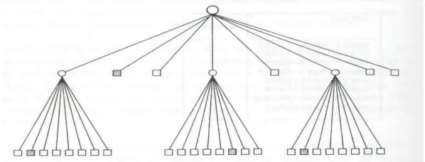
Figure 3.1 Representation of an Object with n=2 (Modified after Gargantini 1989) . . . . 34

Figure 3.2 Octree for Object in Figure 3.1 (Modified after Gargantini 1989) . . . . 34

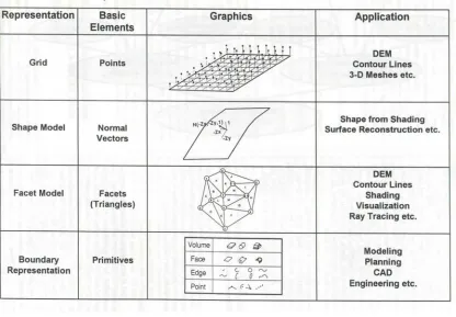
Figure 3.3 Classification of 3-D Geometric Representations (Li 1994) . . . . 41

Figure 3.4 Surface Based 3-D Geometric Representations (Li 1994) . . . . 41

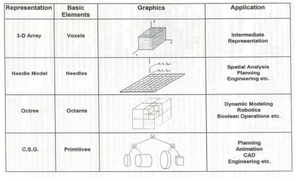
Figure 3.5 Volume Based 3-D Geometric Representations (Li 1994) . . . . 42

Figure 3.6 The Point Model for a Pyramid . . . . 46

Figure 3.7 The Contour Line Model for a Pyramid . . . . 46

Figure 3.8 The DEM for the Pyramid . . . . 47

Figure 3.9 The TIN Model for the Pyramid . . . . 48

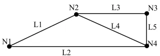
Figure 3.10 A Simple Network Model . . . . 53

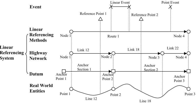
Figure 3.11 Conceptual Overview of the LRS Data Model (Modified after Vonderohe et al. 1995) . . . . 55

Figure 3.12 The Conceptual Model of a Linear Referencing System (Summarized after Vonderohe et al. 1995) . . . . 56

Figure 3.13 Milepost/Milepoint/Reference Post Location Reference Method (Modeled after Geo Decisions 1997) . . . . 57

Figure 3.14 Link-Node Location Reference Method (Modeled after Geo Decisions 1997) . . . . 58

Figure 3.15 X-Y Point Location Reference Method (Modeled after Geo Decisions 1997) . . . . 58

Figure 3.16 Address/Intersection Location Reference Method (Modeled after Geo Decisions 1997) . . . 59

Figure 4.1 Data Quality Parameter Matrix . . . . 70

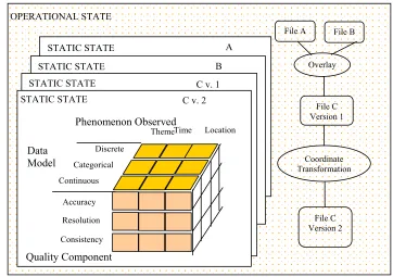
Figure 4.2 Static and Operational States of Data Quality Evaluation (Modeled after Wu and Buttenfield 1994) . . . . 70

Figure 4.3 Measuring Components of Positional Accuracy for Point (Modeled after Veregin 1999) . . . 76

Figure 4.4 The Early Model of Positional Accuracy for Lines (Modeled after Goodchild 1991a) . . . . 77

Figure 4.5 A Practical Error Evaluation Method for Lines . . . . 77

Figure 4.6 Variations in Band Shape and Error Distribution (modeled after Veregin 1999) . . . . 78

Figure 4.7 Illustration of the Dilemma in Determining Positional Accuracy for Polygons . . . . 78

Figure 4.8 The Illustration of New Data Derivation . . . . 83

Figure 4.9 Example of Errors in LRS (Modeled after Miller and Shaw 2001) . . . . 87

Figure 5.1 Add-On Electronic Distance Measuring Instrument Mounted on a Theodolite (Photo Courtesy of Sokkia Corporation) . . . . 90

Figure 5.2 Current Total Station, Trimble 3600 Series (Photo Courtesy of Trimble Navigation Limited) . 90 Figure 5.3 Principles of EDMI Measurement (Courtesy of Kern Instruments-Leica) (Kavanagh 1997) . . 91 Figure 5.4 The Horizontal Plane for Angle Measurement (Schofield 1993) . . . . 93

Figure 5.5 Illustration of Distance Calculation in Total Station (Moffitt and Bossler 1998) . . . . 94

Figure 5.6 Data Collector (Courtesy of Trimble Navigation Limited) . . . . 95

Figure 5.7 Prisms (Courtesy of Topcon Instrument Corp., Paramus, NJ) . . . . 95

Figure 5.8 Plan View Showing Collimation Error (Worawat and Rasdorf 2003) . . . . 96

Figure 5.9 Front View Showing Transit Axis Error (Worawat and Rasdorf 2003) . . . . 96

Figure 5.10 Relation between Angular and Linear Error (Moffitt and Bossler 1998) . . . . 98

Figure 5.11 Approximation of 3-D Distance between Two Locations via Segmentation . . . . 99

Figure 5.12 Three Major Segments of GPS (Source: http://www.aero.org/publications/GPSPRIMER) . . 101

Figure 5.13 Satellite Constellation (Source: http://www.garmin.com) . . . . 101

Figure 5.14 GPS Master Control and Monitor Station Network (Source: Peter H. Dana 5/27/1995) . . . 102

Figure 5.15 Illustration of Multipath Errors (Source: http://www.garmin.com) . . . . 104

Figure 5.16 Hand Wheel (Worawat and Rasdorf 2003) . . . . 107

Figure 5.17 DMI Attached to Car Dash Board (Courtesy of Nu-Metrics) . . . . 107

Figure 5.19 Wheel Sensor (Courtesy of Nu-Metrics) . . . . 109

Figure 5.20 Transmission Sensor (Courtesy of Nu-Metrics) . . . . 109

Figure 6.1 Line Construction in 2-D GIS . . . . 117

Figure 6.2 Line Construction in 3-D GIS . . . . 117

Figure 6.3 A Variation of 3-D Point Model with the Use of LRS . . . . 118

Figure 6.4 An Example of Mathematical Model in the Case of LRS Road Data . . . . 120

Figure 6.5 Illustration of the Basic Structure of a Grid (Modified after Maune et al. 2001) . . . . 126

Figure 6.6 Conversion of NED Data into a Grid File (Modeled after Rasdorf et al. 2003a) . . . . 139

Figure 6.7 Illustration of Electromagnetic Spectrum (Worawat and Rasdorf 2003) . . . . 141

Figure 6.8 Components of a LIDAR System . . . . 141

Figure 6.9 Operation of Airborne LIDAR in Mapping (Courtesy of NC Floodplain Mapping Program) . 141

Figure 7.1 ArcMap Displaying X/Y Coordinates for a Point on a Line . . . . 154

Figure 7.2 Illustration of the Spatial Properties and Spatial Relations for Points and a Linear Object . . 155

Figure 7.3 Three Groups of LIDAR Points Based on the Spatial Relationships . . . . 157

Figure 7.4 Illustration of Obtaining Intersections and Determining Their Elevations . . . . 158

Figure 7.5 Cross-Sectional View of Comparing the Vertical Errors Due to Interpolation and Approximation . . . . 160

Figure 7.6 Comparison of the Interpolation Approach with the Approximation Approach . . . . 161

Figure 7.7 Illustration of the Density of LIDAR Points in Johnston County, North Carolina . . . . . 163

Figure 7.8 Bilinear Interpolation of Obtaining Elevations from DEMs (Rasdorf et al. 2003b) . . . . . 165

Figure 7.9 Obtaining Intermediate Points along a Linear Object . . . . 165

Figure 7.10 Defining Best-Fitting Line . . . . 167

Figure 7.11 Maximum Vertical Adjustments . . . . 169

Figure 7.12 Processing Procedure for 3-D Spatial Modeling and 3-D Distance Prediction when Working with LIDAR Point Data and Road Network Data . . . . 172

Figure 7.13 Processing Procedure for 3-D Spatial Modeling and 3-D Distance Prediction when Working with DEM Data. . . . 173

Figure 8.1 Availability of LIDAR Data in North Carolina . . . . 179

Figure 8.2 Study Scope for the Case Study . . . . 180

Figure 8.3 Detailed View of the Study Scope for the Case Study . . . . 180

Figure 8.4 Digitizing Road Centerlines from DOQQs . . . . 183

Figure 8.5 Illustration of Intersection, Link, and Node . . . . 187

Figure 8.6 Illustration of Errors in Digitizing Linear Features . . . . 188

Figure 8.7 Illustration of Dilemmas in Digitizing Road Centerlines . . . . 189

Figure 8.8 Illustration of Misalignment between Sign Locations and County Lines . . . . 190

Figure 8.9 RMSE Trends . . . . 197

Figure 8.10 Illustration of Errors due to Stopping on Shoulders at Start and End Points . . . . 200

Figure 8.11 Quality Control in Identifying Start or End Points When Collecting DMI Measurements . . 201 Figure 8.12 Algorithm for Deriving FTSegs from Link-Node System . . . . 205

Figure 8.13 Illustration of Reducing the Number of LIDAR Points by Applying a Buffer – Part I . . . 206

Figure 8.14 Illustration of Reducing the Number of LIDAR Points by Applying a Buffer – Part II . . . 207

Figure 8.15 An Illustration of the Algorithm for Snapping . . . . 209

Figure 8.16 Illustration of the Dilemma in Determining Elevations for Start and End Points . . . . 211

Figure 8.17 Illustration of Sample Results from Snapping . . . . 211

Figure 8.18 Illustration of Interpolation, Extrapolation, and Weighted Average Scenarios for End Points . 213 Figure 8.19 Illustration of Connected FTSegs with Different Road Types . . . . 214

Figure 8.20 An Example of 3-D Points Simulating the Road Centerline . . . . 215

Figure 8.21 Illustration of Suspect Points . . . . 216

Figure 8.22 Illustration of a Typical Scenario Associated with Suspect Points . . . . 217

Figure 8.23 Illustration the Scenario for Further Improvement . . . . 218

Figure 8.24 Algorithm of Working with LIDAR DEMs . . . . 221

Figure 9.4 Distribution Histograms (LIDAR Point Data, Proportional Differences) . . . . 244

Figure 9.5 Distribution Histograms (LIDAR 20-ft DEM, 10-ft Interval, Differences) . . . . 245

Figure 9.6 Distribution Histograms (LIDAR 20-ft DEM, 10-ft Interval, Proportional Differences) . . . 245

Figure 9.7 Distribution Histograms (LIDAR 20-ft DEM, 20-ft Interval, Differences) . . . . 246

Figure 9.8 Distribution Histograms (LIDAR 20-ft DEM, 20-ft Interval, Proportional Differences) . . . 246

Figure 9.9 Distribution Histograms (LIDAR 50-ft DEM, 25-ft Interval, Differences) . . . . 247

Figure 9.10 Distribution Histograms (LIDAR 50-ft DEM, 25-ft Interval, Proportional Differences) . . . 247

Figure 9.11 Distribution Histograms (LIDAR 50-ft DEM, 50-ft Interval, Differences) . . . . 248

Figure 9.12 Distribution Histograms (LIDAR 50-ft DEM, 50-ft Interval, Proportional Differences) . . . 248

Figure 9.13 Distribution Histograms (NED, 15-m Interval, Differences) . . . . 249

Figure 9.14 Distribution Histograms (NED, 15-m Interval, Proportional Differences) . . . . 249

Figure 9.15 Distribution Histograms (NED, 30-m Interval, Differences) . . . . 250

Figure 9.16 Distribution Histograms (NED, 30-m Interval, Proportional Differences) . . . . 250

Figure 9.17 Comparisons of 100% Sample Means of Differences . . . . 281

Figure 9.18 Comparisons of 100% Sample Means of Proportional Differences . . . . 283

Figure 9.19 Comparisons of 95% Sample Means of Differences . . . . 284

Figure 9.20 Comparisons of 95% Sample Means of Proportional Differences . . . . 285

Figure 9.21 Comparison of Medians of Differences . . . . 286

Figure 9.22 Comparison of Medians of Proportional Differences . . . . 287

Figure 9.23 Comparison of 100% Absolute Means of Differences . . . . 289

Figure 9.24 Comparison of 95% Absolute Means of Differences . . . . 290

Figure 9.25 Comparison of 100% Absolute Means of Proportional Differences . . . . 291

Figure 9.26 Comparison of 95% Absolute Means of Proportional Differences . . . . 292

Figure 9.27 Comparison of 100% RMSEs for Differences . . . . 294

Figure 9.28 Comparison of 100% RMSEs for Proportional Differences . . . . 295

Figure 9.29 Comparison of 95% RMSEs for Differences . . . . 296

Figure 9.30 Comparison of 95% RMSEs for Proportional Differences . . . . 297

Figure 9.31 Illustration of Percentages at the Error Range of [-5, 5] for Differences . . . . 299

Figure 9.32 Illustration of Percentages at the Error Range of [-10, 10] for Differences . . . . 300

Figure 9.33 Illustration of Percentages at the Error Range of [-20, 20] for Differences . . . . 301

Figure 9.34 Illustration of Percentages at the Error Range of [-30, 30] for Differences . . . . 303

Figure 9.35 Illustration of Percentages at the Error Range of [-50, 50] for Differences . . . . 304

Figure 9.36 Illustration of Percentages at the Error Range of (-∞, -50) and (50, +∞) for Differences . . . 305

Figure 9.37 Illustration of Percentages at the Error Range of [-1, 1] for Proportional Differences . . . . 306

Figure 9.38 Illustration of Percentages at the Error Range of [-5, 5] for Proportional Differences . . . . 307

Figure 9.39 Illustration of Percentages at the Error Range of [-10, 10] for Proportional Differences . . . 308

Figure 9.40 Illustration of Percentages at the Error Range of [-20, 20] for Proportional Differences . . . 309

Figure 9.41 Illustration of Percentages at the Error Range of [-30, 30] for Proportional Differences . . . 310

Figure 9.42 Illustration of Percentages at the Error Range of [-50, 50] for Proportional Differences . . . 311

Figure 9.43 Illustration of Percentages at the Error Range of [-100, 100] for Proportional Differences . . 312 Figure 9.44 Illustration of the Effects from the Point Positional Errors on the Predicted 3-D Distances . . 314 Figure 9.45 Illustration of the Effects of the 3-D model on the Predicted 3-D Distances . . . . 314

Figure 9.46 Illustration of the Difference between the True 3-D Line and the Constructed 3-D Line . . 315

Figure 10.1 Illustration of Slope and Slope Change Calculation . . . . 322

Figure 10.2 The Algorithm of Calculating Average Slopes, Weighted Average Slopes, Slope Changes, and Weighted Slope Changes . . . . 324

Figure 10.3 Comparison of RMSEs of the Difference for Groups Based on the Distance . . . . 344

Figure 10.4 Comparison of RMSEs of the Proportional Difference for Groups Based on the Distance . . 345 Figure 10.5 Comparison of RMSEs of the Difference for Groups Based on the Average Slope . . . . . 347

Figure 10.6 Comparison of RMSEs of the Proportional Difference for Groups Based on the Average Slope . . . . 348

Figure 10.7 Comparison of RMSEs of the Difference for Groups Based on the Weighted Average Slope . . . . 351

Figure 10.8 Comparison of RMSEs of the Proportional Difference for Groups Based on the Weighted Average Slope . . . . 352

Figure 10.10 Comparison of RMSEs of the Proportional Difference for Groups Based on the Average Slope

Change . . . . 355

Figure 10.11 Comparison of RMSEs of the Difference for Groups Based on the Weighted Average Slope Change . . . . 357

Figure 10.12 Comparison of RMSEs of the Proportional Difference for Groups Based on the Weighted Average Slope Change . . . . 358

Figure 10.13 Comparison of RMSEs of the Difference and Proportional Difference for Groups Based on the Number of 3-D Points . . . . 360

Figure 10.14 Comparison of RMSEs of the Difference and Proportional Difference for Groups Based on the Average Density of 3-D Points . . . . 362

Figure 11.1 Modeling Water Bodies Using Polylines . . . . 369

Figure 11.2 Cross-sectional View of Flooding . . . . 369

Figure 11.3 Illustration of Flooded and Not Flooded Road Segments in the Flooded Area . . . . 370

Figure 11.4 Conceptual Model for Predicting Flood Extent . . . . 372

Figure 11.5 Conceptual Model for Identifying Flooded Road Segments . . . . 373

Figure 11.6 Obtaining Points along A Polyline . . . . 376

Figure 11.7 The Procedure of Predicting Flood Extent . . . . 377

Figure 11.8 Identifying Points with Target Elevation . . . . 378

Figure 11.9 Illustration of Water Flow . . . . 379

Figure 11.10 Error Tolerance and Maximum Drop . . . . 380

Figure 11.11 Flood Road Segment Identification Algorithm, Part I . . . . 382

Figure 11.12 Flood Road Segment Identification Algorithm, Part II . . . . 383

Figure 11.13 An Illustration of Identifying Flooded Road Segment Algorithm . . . . 384

Figure 11.14 Study Scope for Testing in Wilson County . . . . 385

Figure 11.15 Testing Results – Algorithm 1 . . . . 386

Figure 11.16 Testing Results – Algorithm 2 . . . . 386

Figure 11.17 Detailed View – Algorithm 1 . . . . 386

Figure 11.18 Detailed View – Algorithm 2 . . . . 386

Figure 11.19 Flooded Road Segments – Algorithm 1 . . . . 388

Figure 11.20 Flooded Road Segments – Algorithm 2 . . . . 388

1

INTRODUCTION AND BACKGROUND

This chapter describes briefly the development and definition of geographic information systems (GISs), their

applications in various fields, the basics of geographic modeling and data structure, data quality issues, and

geographic information systems in transportation (GIS-T). Section 1.6 (Research Needs) states the motivation

for this research. Terms and terminologies being used are also defined in this chapter. In addition, section 1.8

summarizes the organization of this dissertation to provide better understanding.

1.1 BACKGROUND

Human beings started to locate themselves on the Earth and navigate along the Earth surface in the very early

years. It is known that human beings put stones on the ground to help them keep track of their routes and had

relied on the stars in the sky to help locate their positions. The spatial information was so valuable that people

tried to record this information even before the emergence of paper and compass. The competition for and

demands on natural resources of land, air, water, and raw materials accompanying civilization brought the needs

to record land use, land ownership, and transactions in a way that is not dependent on human memories

(Burrough and McDonnell 1998).

From the earliest civilization to modern times, the above-mentioned spatial data have been collected by

navigators, geographers, and surveyors to be recorded in a coded, pictorial form by mapmakers and

cartographers (Burrough and McDonnell 1998). It is known that the land surveyors were an important part of

the government in Roman times and that the results of their work may still be seen in vestigial form in the

European landscapes to this day (Dilke 1971). By the seventeenth century skilled cartographers such as

Mercator had demonstrated that the registration of spatial phenomena through an agreed standard provided a

model of the distribution of natural phenomena and human settlements that were invaluable for navigation,

route findings, and military strategies (Hodgkiss 1981). Cartographers recorded the locations and

characteristics of natural phenomena using a powerful range of tools. Point and line symbols were chosen to

represent the most important characteristics of the objects while areas were colored differently to represent the

Today, much geographical information concerns the location of well-defined objects in space and the

interactions among them (Burrough and McDonnell 1998). Examples include trees in a forest, roads connecting

cities, and houses on a street. Spatial data and spatial analyses are being widely used in a variety of fields.

Civil engineers use them to plan the routes of roads and to estimate construction costs. Police departments need

to know crime distribution and to determine emergency routes. The utility companies need to record the

positions and locations of the utility systems. The urban planners need detailed information about the

distribution of land and resources in towns and cities. Foresters are interested in the distribution of trees. All

these applications reveal that using traditional paper maps to record geographical information have several

severe drawbacks that make them inappropriate in these applications. These drawbacks include:

• In order to represent spatial data in paper maps, the original data had to be greatly reduced and

consequently, many details were often filtered away and thus lost.

• The information for large areas with respect to map scale could only be represented by a number of map

sheets. It is not uncommon that the interested areas are near the junctions of two or more maps.

• Once the paper map is produced, it is very difficult and costly to make changes or to be combined with

other spatial information.

• Most importantly, paper maps are just static and qualitative documents. Spatial analyses that deal with the

interactions of spatial objects are extremely difficult with these paper maps.

More recently, using aerial photographs and satellite images enables monitoring landscape changes over time

and provides an efficient way to obtain useful information about the Earth’s surface. However, the products of

the airborne and space sensors are not maps, rather, they are images. The digital data of these products are not

in the form of points, lines, or polygons as in traditional maps. There is a need for the integration of remote

sensing, Earth-bound survey, and cartography. This is only made possible by the class of spatial information

handling and mapping tools known as geographic information systems (GISs).

heavily computer oriented (Burrough and McDonnell 1998). GISs model spatial objects and their relationships

in a consistent manner and carry out spatial analyses efficiently; therefore, GISs overcome the drawbacks of the

traditional maps.

By the late 1970s there had been considerable investments in the development and application of

computer-assisted cartography, particularly in North America by government and private agencies (Burrough and

McDonnell 1998). With more than twenty years of technical development in GISs, they are becoming a

worldwide phenomenon. In 1995 it was estimated that more than 93,000 sites worldwide had installed GISs

(Burrough and McDonnell 1998). Today, GISs are being utilized in various fields including agriculture,

archaeology, Earth observations, epidemiology and health, forestry, emergency services, navigation, marketing,

real estate, regional/local planning, transportation, social studies, natural resource management, land use and

land cover mapping, hydrology, civil engineering, mining, geology, geography, soil science, and much more.

1.2 GIS

The concept of GISs traces its roots to a handful research initiatives in the US, Canada, and Europe during the

1950s (Thill 2001). The first real GIS was the Canada Geographic Information System set up for the Canada

Land Inventory.

A GIS may be defined as a computer-based tool set for collecting, storing, retrieving, transforming and

displaying spatial data from the real world for a particular set of purposes (Burrough 1986). A GIS has at least

five components: people, data, hardware, software, and procedures.

A GIS works with spatial data. Spatial data represent phenomena from the real world in terms of (1) their

positions with respect to a known coordinate system, (2) their attributes that are unrelated to position (examples

include thickness, cost, incidence of accidents, and etc.), and, (3) their spatial interrelations with each other

which describe how they are linked together (this is known as topology and describes space and spatial

From a functional point of view, a GIS must be able to realize at least four tasks (Rasdorf and Cai 2001).

(1) Data input and verification,

(2) Data storage and database management,

(3) Data output and presentation, and

(4) Data transformation.

It is the functional complexity of GISs that differentiates a GIS from any other systems. The geo-visualization

capability differentiates a GIS from a database management engine. The analytical capability differentiates a

GIS from automated mapping applications (Thill 2000). On the other hand, the database management features

in GISs enable GISs to capture spatial and topological relationships between geo-referenced entities without

pre-defining these relationships (Thill 2000).

1.3 2-D, 2.5-D, AND 3-D MODELING

As indicated by the name, a GIS works with geographic data, which can be understood as the information tied

to some portion of the Earth (Chrisman 2002). It is obvious that we do not store real world phenomena in the

computer but only representations of these phenomena based on some formalized models (Burrough and

McDonnell 1998). In other words, a model can be defined as a set of rules to abstract real world phenomena

while modeling can be defined as the procedure of abstracting real world phenomena so that representations are

produced. In the case of GISs, modeling enables us to obtain geographic information to describe those real

world phenomena. It is this information that is being input into and stored in the computer and analyzed to

support decision-makings.

Geographical phenomena require two descriptors to represent the real world, what is present and where it is

(Burrough and McDonnell 1998). Geographic information is commonly broken into three components: space,

time, and attribute. It requires reference systems, which are defined as a set of rules for measurement and

A spatial reference system can be defined as a mechanism to situate measurements on a geometric body. It

establishes a point of origin, orientation of reference axes, and geometric meaning of measurements and units of

measurements (Chrisman 2002).

As outlined earlier, modern GISs are developed based on the concepts that have been well established with the

emergence and development of paper mapping. The basic spatial models used in modern GISs are little

different from those used 15-20 years ago (Burrough and McDonnell 1998). All real world spatial objects exist

in Euclidean 3-D space (Smith and Paradis 1989). Paper mapping spatially locates three dimensional real world

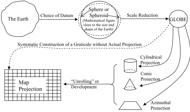
objects in a two-dimensional coordinate system, more specifically, an X and Y coordinate system. Figure 1.1

illustrates the procedure of map projections to convert three dimensional objects on Earth surface into two

dimensional coordinate systems. This procedure is being followed by most geographic information systems on

market.

Figure 1.1 The Procedure of Map Projections

The actual shape of the Earth is too lumpy to use as a reference surface. The first step is to adopt a model for

the Earth, usually in the form of a reference ellipsoid. Examples include Clarke’s 1866 and WGS 84. Then a

geodetic datum is developed for the Earth using the established longitude-latitude format. The Earth’s surface Choice of Datum

The Earth

Sphere or Spheroid

(Mathematical figure close to the size and

shape of the Earth)

GLOBE

Scale Reduction

Map

Projection

Systematic Construction of a Graticule without Actual Projection

“Unrolling” or Development

Cylindrical Projection

Conic Projection

is not flat. In order to place objects on a two-dimensional plane, a procedure called projection is required. A

projection transforms latitude-longitude information into planar coordinates, resulting in map construction on

two-dimensional media in Cartesian coordinate systems. After projection, the origin point, axis directions, and

measurement units are determined and a spatial reference system is developed.

2-D modeling captures the planimetric positions of objects on a two-dimensional plane. Most commercially

available GIS products take this approach and therefore, cannot handle true 3-dimensional data, although they

can handle topographic data, usually as a digital elevation model (DEM), and display isometric views, contour

maps and so on (Turner 1989a, 1989b, 1989c, and 1989d). Most DEMs use either grid elevation matrices, or

triangular meshes (TINs) to allow for terrain representations. This is enabled by treating the elevation, or the

third dimension (Z-coordinate) as a dependent variable. This approach is defined as the quasi-

three-dimensional, or 2.5-D modeling approach. In other words, the dependence of Z-coordinate on the X- and

Y-coordinates in the 2.5-D approach enables deriving Z values using X and Y values and some supplementary

information, and employing some interpolations or mathematical functions. In the 2.5-D approach, only one

elevation value is allowed for a specific pair of X/Y-coordinates.

Different from 2-D and 2.5-D modeling approaches, 3-D modeling represents spatial objects in a true

three-dimensional space. The 3-D modeling approach treats the third dimension (or Z-coordinate) as an independent

variable. Figure 1.2 illustrates the differences in representing a simple linear object in 2-D, 2.5-D, and 3-D

spaces. In the 3-D space, the object might not be a simple linear object as illustrated in Figure 1.2.

Figure 1.2 The Differences in Representing a Linear Object in 2-D, 2.5-D, and 3-D spaces

Y

X Y

X

Y

X Z

2-D modeling represents the object in a 2-D space

2.5-D modeling represents the object in a 2-D space, elevations can be derived from the underlying elevation grid

1.4 DATA QUALITY

Data quality is a critical feature of successful use of GISs, whether working in two dimensions or three

(Burrough 1986, Burrough and McDonnell 1998, Rhind 1981). Data quality is an important factor to any

information systems whose goal is to effectively and accurately convey information. The Federal Geographic

Data Committee (FGDC) has been working on data quality standards for years. One of its outcomes, the US

Spatial Data Transfer Standard (SDTS 1997), addresses this subject as follows.

“Quality is an essential or distinguishing characteristic necessary for cartographic data to be fit for use.”

The quality of data is one of the most important factors for information systems that are intended to conduct

analysis and support decision-makings. It is clearly recognized that the validity of analysis is based on the

validity of the data used to perform the analysis (Rasdorf et al. 2001). Any geographic data are an abstraction

of the real-world phenomena they represent. It is not always the case that a phenomenon can be exactly

visualized, understood, and modeled in an information system. In other words, errors and deviations are

inherent in information management systems, which lead to the necessity for data quality control (Rasdorf et al.

2001).

1.5 GIS-T AND ROAD CENTERLINE

GISs have benefited the field of transportation for many years due to the rich spatial data in transportation

(Fletcher 1987, Nyerges and Dueker 1988, Dueker and Kjerne 1989, Ries 1993, Vonderohe et al. 1993, Dueker

and Butler 1998, Fletcher 2000). In the transportation context, three classes of GIS models are relevant

(Goodchild 1992, 1998).

• Field models to represent the continuous variation of a phenomenon over space. Terrain elevation uses

this model.

• Discrete models to represent discrete entities (points, lines, and polygons) in space. Highway rest areas,

toll barriers, urbanized areas may use this model.

Among these three relevant models, the network model built around the concepts of arc and node plays the most

prominent role in transportation applications because single- and multi-modal infrastructure networks are vital

in enabling and supporting passenger and represent data (Thill 2000). Many transportation applications only

require network representation of data. Examples include pavement management systems, routing applications,

traffic information systems, congestion management, accident detection, etc.

However, the network model in the conventional GISs assumes the homogeneity of each network link, which

does not hold in transportation. The road parameters such the number of lanes and pavement width cannot be

constrained to be constant between terminal nodes of a link. Also, traffic parameters of speed, flow and

capacity cannot be expected to be constant along a link. The dynamic nature of these distributed attributes of

the network precludes that the network be permanently edited to maintain the homogeneity of each link on each

attribute, which leads to the concept of linear referencing (Thill 2000). In the linear referencing approach,

attributes are linearly referenced and linked dynamically to the entities forming the network (Scarponcini 1999).

This capability of geographic information systems in transportation (GIS-T) was identified as critical in the

early researches in GIS-T (Dueker 1987, Fletcher 1987, Vonderohe et al. 1993).

To summarize, GIS in transportation is more than just one more domain of application of generic GIS

functionality because GIS-T has several data modeling, data manipulation, and data analysis requirements that

are not fully supported by conventional GISs (Thill 2000). Rather, it is viewed as the cross-fertilization of an

enhanced GIS and an enhanced transportation information system (TIS) as illustrated in Figure 1.3 (Vonderohe

et al. 1993).

Figure 1.3 GIS-T, Product of an Enhanced GIS and an Enhanced TIS (Vonderohe et al. 1993)

GIS

TIS

highway geometric design, i.e. the sight distance, cross section, horizontal alignment, super elevation, vertical

alignment, channelization, and pavement design, the cross section, the horizontal alignment, and the vertical

alignment together depict the roads spatially as surface objects.

Cross section design refers to the profile of the facility that is perpendicular to the centerline and extends to the

limits of the right-of-way within which the facility is constructed (Papacostas and Prevedouros 2001). The

cross section of road includes the pavement, shoulder, clear zone, and additional R/W as required. The

horizontal alignment represents the projection of the road facility on a horizontal plane. It generally consists of

straight-line segments (tangents) connected by circular curves directly (simple curves) or via intermediate

transition curves (Papacostas and Prevedouros 2001). The vertical alignment of highways and railways consists

of grade tangents connected with parabolic vertical curves. Figure 1.4 illustrates the concepts of horizontal

alignment and vertical alignment with a straight road segment connected directly to a circular segment. Figure

1.5 illustrates a typical cross s