An Algorithm for Determining Optimal Resource Allocation in Stochastic Activity Networks

Abstract

RUDOLPH, ADAM J. An Algorithm for Determining the Optimal Resource Allocation in  Stochastic Activity Networks.  (Under the direction of Professor Salah E. Elmaghraby). 

The problem we investigate deals with the optimal assignment of resources to the 

activities of a stochastic project network.  We seek to minimize the expected cost of the 

project, which we take as the sum of resource utilization costs and lateness costs, if the 

project is completed after a specified due date.  These costs are both functions of the resource 

allocations to the activities with opposite responses to changes in allocation.  We assume that 

the work content required by the activities follows an exponential distribution.  An 

immediate result of this assumption is that the duration of the activities also follows an 

exponential distribution based on the degree of resource allocation.  We construct a 

continuous time Markov chain (CTMC) model for the activity network and use the Phase­ 

Type (PH­type) distribution to evaluate the project completion time. 

Absence of an analytically tractable means of evaluating the sensitivity of the project 

cost to variation in the resource allocation to an individual activity led us to develop a 

derivative descent algorithm for the optimization of the expected cost of the project.  We 

approximate the value of the derivative at a particular allocation by evaluating the differential 

cost of a slightly modified allocation.  These quasi­derivatives led to the selection of an 

activity to which we optimize resource allocation.  We use Fibonacci search over the interval 

of permissible allocations to the activity to seek the minimum expected cost.  This iterative 

process of activity selection followed by changing the resource allocation is repeated until 

the expected cost is not significantly decreased.  Finally, through extensive experimentation 

with a variety of projects of different structure and size, we show that this algorithm yields 

An Algorithm for Determining the Optimal Resource  Allocation in Stochastic Activity Networks 

by 

Adam J. Rudolph 

A thesis submitted to the Graduate Faculty of  North Carolina State University 

In partial fulfillment of the  Requirements for the Degree of 

Master of Science 

Operations Research 

Raleigh, North Carolina  May 2008 

APPROVED BY: 

__________________________________  Dr. Subhashis Ghosal 

__________________________________  Dr. Julie Ivy 

__________________________________  Dr. Salah E. Elmaghraby 

Biography

Adam Rudolph was born on December 5 of 1983 in Louisville, Kentucky, however 

most of his childhood was spent in Lafayette, Indiana.  He enrolled at Purdue University in 

West Lafayette, Indiana in August of 2002 where he studied Industrial Engineering and was 

introduced to the field of Operations Research.  While at Purdue, Adam had the opportunity 

to pursue internships with H.B. Maynard and Co., Caterpillar Inc., and GE Healthcare.  He 

graduated from Purdue in May of 2006. 

Adam moved to Raleigh, North Carolina and enrolled at North Carolina State 

University in August of 2006 to pursue a graduate education in Operations Research.  He will 

Acknowledgements

I would like to express my thanks to Dr. Salah E. Elmaghraby, Dr. Julie Ivy, and Dr. 

Subhashis Ghosal for their hard work and dedication as my advisory committee.  Through 

their time and help they have assisted me greatly in the completion of my thesis.  I would 

also like to thank our department secretary Barbara Walls for her assistance with the many 

administrative details throughout my time at NCSU. 

I must also thank Dr. Demeulemeester of Katholieke Universiteit Leuven for his 

provision of the RanGen and RanGen2 network generators. 

Personally, I must thank my family, Ed and Sheila Rudolph and Sara and Jerod 

Patterson for their prayers and support throughout my formal education, graduate and 

otherwise. 

There are so many others I could mention for countless simple acts of support that 

have made the completion of this graduate degree possible.  Thank you to my many teachers, 

friends, and family who have been there for me throughout my life and especially thanks to 

Table of Contents

List of Tables ... vi 

List of Figures ... vii 

Introduction...1 

Literature Review ...3 

2.1  Project Scheduling and PERT networks ...3 

2.2  Continuous Time Markov Chains...7 

2.3  Relevant Recent Studies:...8 

Problem Statement ...10 

3.1  Introductory Assumptions ...10 

3.2  Continuous Time Markov Chains...14 

3.3  Phase­Type Distributions ...18 

3.4  The Cost Function...21 

Description of Algorithm...22 

4.1  Cost Computation ...22 

4.2  Selecting Candidate Activities...25 

4.3  Improving Computational Efficiency ...27 

4.4  Optimizing The Allocation to a Single Variable ...28 

4.5  Stopping Criteria...31 

4.6  An Illustrative Example ...32 

Results ...35 

5.2  Network Structure Considerations...39 

Conclusions and Future Research ...44 

6.1  Conclusions ...44 

6.2  Directions for Future Research...46 

Bibliography ...51 

Appendix A: Test Network Generation...54 

List of Tables

Table 1: State Space of the CTMC...16 

Table 2: Example Derivative Approximation...33 

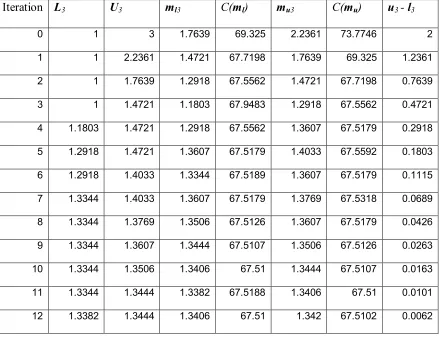
Table 3: Fibonacci Search Procedure Example ...34 

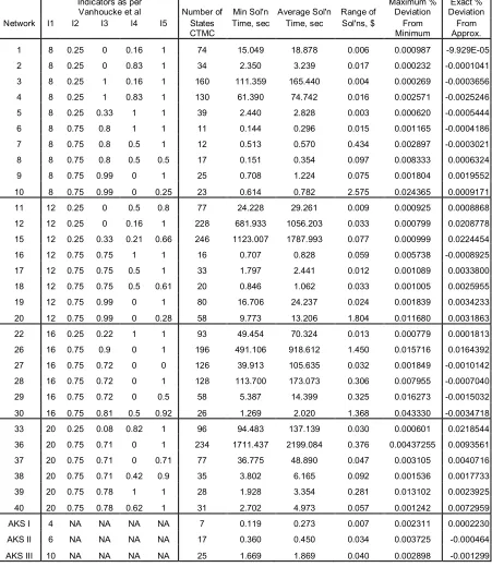
Table 4: Test Results ...36 

Table 5: Example Network Test Results ...43 

Table 6: State Space of the AoN Example Network...57 

List of Figures

Figure 1: An Example 3­Activity Network ...10 

Figure 2: The State Space of the Project of Figure 1: ...17 

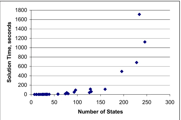
Figure 3: Solution Time vs Number of States in CTMC...38 

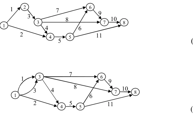
Figure 4: Example Network 2...41 

Figure 5: Example Network 2 with Reduced Complexity ...41 

Figure 6: Example Network 2 with Further Complexity Reduction...42 

Figure 7: Series­Parallel Network...42 

Chapter 1 

Introduction

In many modern business, engineering, and industrial environments, reliable project 

scheduling tools are invaluable.  Predictions of project completion dates and project costs 

strongly impact many business decisions.  In turn, these decisions can impact the course of 

the coming weeks, and often years, for modern companies.  As a result, it is important to 

have accurate predictions of project costs and completion times for management to make the 

best, most informed decisions. 

Much of the literature pertaining to project scheduling problems ignores the simple 

fact that activity durations within a project framework are not known with certainty.  This 

fact can strongly impact the validity of project planning tools in real life applications. 

Further, many project scheduling problems deal with ordering the various tasks of the project 

in such a way to meet some predefined objective.  In reality, often a project manager has 

several resources at his or her disposal that can be used to complete a multitude of project 

tasks that can be undertaken at a particular point in time.  Keeping this in mind, we seek to 

develop a model and create an algorithm that will find the optimal way to assign resources to 

the various stochastic activities of a project to minimize an economic objective function. 

In the next chapter we discuss the literature that is available pertaining to project 

scheduling.  We review several papers regarding classical project scheduling problems and 

Markov Chain representations of projects.  We then discuss in more depth a few papers that 

are closely related to the research at hand.  In Chapter 3 we formally state the problem under 

arrive at a formal statement of our economic objective function.  Chapter 4 contains a 

complete description of the optimizing algorithm.  We pay special attention to a few 

simplifying assumptions that lighten the computational burden required and include 

illustrative examples to aid comprehension.  In Chapter 5 we present the key results of our 

research as obtained from testing our algorithm on a set of test networks and discuss the 

computational burdens imposed by certain network structures.  We conclude by discussing 

several possible extensions to the work presented in this thesis.  In Appendix A, we briefly 

describe the methodology employed in the generation of test networks.  Finally, in Appendix 

B we list the scripts used in MATLAB to optimize resource allocation to the activities of 

these test project networks.  These scripts are detailed at length to assist in verifying our 

results and to provide a basis for extension to future research in any of the directions 

Chapter 2 

Literature Review

This review is categorized into three sections.  First we briefly survey the literature within the 

realm of project scheduling and activity networks in both deterministic and stochastic 

settings.  Second, we summarize the relevant concepts in continuous time Markov chains, 

Markov PERT Networks and the advantages afforded by their application.  Finally, we 

discuss several recent research projects that have studied problems similar to our own. 

2.1  Project Scheduling and PERT networks 

A great deal of research has been done pertaining to project scheduling since the 

field’s inception.  Classically, CPM (“critical path method”) and PERT (“program evaluation 

and review technique”) models have been the industry standard for some time both for their 

effectiveness and for their simplicity.  In the traditional sense, however, neither model takes 

resource constraints into account as they opt to deal more with precedence relationships and 

time considerations.  More recently, much effort has been spent researching the Resource 

Constrained Project Scheduling Problem (RCPSP) which we look into briefly before 

discussing the stochastic case. 

The objective of the RCPSP studies is to schedule activities in such a manner to meet 

resource availability and precedence constraints in order to optimize an objective function 

unimodal and multimodal cases.  The unimodal case involves preset durations and resource 

requirements for each activity, whereas the multimodal case allows activities to be processed 

in a number of different “modes” requiring different resource levels and completion times. 

Resource constraints can be classified as renewable or nonrenewable.  Renewable resource 

constraints put limits on the amount of a particular resource that can be utilized at a particular 

time in the project.  Non­renewable resource constraints limit the amount of a particular 

resource that can be utilized in total throughout the project’s life. Chapters 7 through 9 of 

Demeulemeester and Herroelen [2002] provide an excellent review of RCPSP problems and 

related optimization techniques. 

The multimodal RCPSP is closely related to the problem at hand.  These problems are 

often referred to as Time­Cost Tradeoff problems (TCTP).  At its core, the TCTP assumes 

that the duration of an activity is a function of the resources assigned to its completion. 

Further, both rely heavily on the concept of “work content”.  Normally, greater resource 

allocation will demand a greater expense, thus we have a tradeoff between the time to 

complete a project and its cost (a function of the resources assigned).  When the task duration 

is a linear function of the assigned resources we have the Linear Time Cost Tradeoff (LTCT) 

problem.  Notably, Fulkerson [1961] studied this problem under the objective of minimizing 

project cost subject to completion before a due date.  He then solved the problem through the 

clever use of primal­dual concepts in linear programming and developed an approach to 

compute the complete cost curve of the project as a function of the project’s due dates. 

If the resource’s allocation is limited to distinct values we have the Discrete Time­ 

Cost Tradeoff (DTCT) problem.  Hindelang and Muth [1979] developed a dynamic 

corresponding AoA project graph is series­parallel.  In the case where the graph is not series­ 

parallel De et al [1997] provide an update to the DP algorithm of Hindelang and Muth.  In 

the same article, they show that the DTCT problem is, in general, strongly NP­Hard by 

reduction from 3SAT. 

Deckro et al [1994] discuss the nonlinear case of the TCTP.  They deviate from the 

traditional approach to the problem which would involve piecewise linearization and suggest 

a true nonlinear program.  Presenting a quadratic program they suggest solution using 

commercially available software.  The authors also investigate some extensions to the model 

including a goal­programming formulation. 

When elements of the project are not known deterministically, analysis of the project 

network becomes much more difficult.  The dearth of literature on the topic is perhaps good 

evidence of this fact.  Even so, several studies have been performed both in the single and 

multiple mode fields. 

Golenko­Ginzburg and Gonik [1997] investigate the RCPSP when faced with 

stochastic activity times.  They use Beta, Normal, and Uniform distributions for activity 

times and determine a heuristically achieved best solution to the problem of minimizing the 

project's expected completion time.  They schedule start times for tasks and proceed 

heuristically.  The authors face the problem of deciding between “entering variables” (the 

activities to be initiated at a particular state of the project) by first using simulation to 

determine the probability that the activity is on the critical path and then solve a 0­1 

Knapsack Problem. 

In another paper, Stork [2001] takes an in­depth look at the RCPSP in the stochastic 

briefly discusses the Linear Time­Cost Tradeoff problem and shows it is NP­hard when 

AND/OR constraints are present.  He further investigates branch­and­bound, forbidden set, 

and priority based procedures for optimization in their relationship to the “robustness” of a 

solution. 

Valls et al. [1998] study the RCPSP with some activities facing stochastic 

interruptions and processing times.  They deal with the concept of Stochastic Programming 

versus Robust Optimization and state the burdens to computation imposed by multiple stages 

Stochastic Programming.  Optimizing the weighted tardiness of either each activity or the 

total project, the authors propose and validate a meta­heuristic solution that blends Tabu 

Search and Scatter Search techniques. 

Wollmer [1985] studies a version of the LTCT problem with an additional stochastic 

parameter.  He deals with the problem where activity durations have a component that is a 

linear function of the allocation plus a random element.  The author first seeks to find the 

minimum required investment subject to an expected project completion time and then solves 

the dual problem of finding the minimum expected completion time subject to a budget 

constraint.  The author utilizes a cutting plane technique for his solutions. 

Gutjahr et al. [2000] consider scheduling problems similar to our own.  However, in 

their approach activities can have one of two possible distributions depending on whether or 

not a project is crashed.  In this vein, our problem may be considered one in which projects 

can be "crashed" to varying degrees (i.e. depending on the allocation of resource to task). 

They are also under the discrete time assumptions but depending on the degree of 

discretization this assumption is overcome.  Further, they define an “HS­Branch­and­Bound” 

success using this approach as opposed to Total Enumeration, or pure Stochastic Branch­and­ 

Bound.  They suggest using different heuristics in different applications. 

2.2  Continuous Time Markov Chains 

In this thesis, we assume that the work content of any task is an exponentially 

distributed random variable.  As a direct result of this assumption, activity durations are also 

exponential random variables since the duration is derived from the work content via the 

relation Y = W/x, in which W is the (random) work content and x is the resource allocation. 

Further, when we assume independence of activity times with respect to one another we have 

a Markov PERT Network (MPN).  Under this assumption the analysis of project networks is 

greatly aided by the use of Continuous Time Markov Chain (CTMC) theory.  A good 

introduction to Continuous Time Markov Chains is provided in Ross [2002]. 

The term Markov PERT Network originated with Kulkarni and Adlakha [1986] and 

refers to stochastic activity networks where activity times follow an exponential distribution. 

Kulkarni and Adlakha [1986] describe Markov PERT Networks in great detail.  Further, they 

provide a method for analysis involving uniformly directed cutsets (UDC’s) that allows one 

to transform the PERT network into a Continuous Time Markov Chain.  An exposition of 

this process will be provided with appropriate definitions in section 3.2 below.  The authors 

then develop recursive formulas for obtaining the moments of the completion time of a MPN. 

Though the use of these formulas is beneficial in certain applications (such as in bounding 

the completion time of the project), we instead favor the use of the Phase­type (PH­type) 

project completion time but also in its distribution based on the project parameters.  We will 

develop the key concepts regarding this distribution in section 3.3. 

2.3  Relevant Recent Studies: 

A few studies have been conducted recently that are in a similar vein to the research 

considered here.  However, they differ from our study in the objective, the optimization 

methodology, or the constraining set. 

Tereso, Araújo, and Elmaghraby [2004] investigate optimal resource allocation under 

stochastic conditions.  They optimize the same objective with which we are faced and relax 

the assumption that work content follows an exponential distribution.  They solve the 

problem using a Dynamic Programming algorithm that is extremely taxing computationally. 

Their approach optimizes the allocation to resources along a single path through the network 

from start to finish while holding the allocations to other activities constant.  Their solution 

necessitates enumerating the optimal path for all possible values of allocations to other 

variables.  In conclusion they suggest treating only exponential distributions which gives rise 

to the research presented in this thesis. 

Morgan [2006] derives a fast method for optimizing resource allocation in a single 

stage stochastic activity network.  He justifies optimizing a single stage by suggesting that a 

project manager’s strategy should change once the state of the project changes as evidenced 

by the completion of an activity.  Morgan uses Sample Path Optimization and appeals to 

Geometric Programming to solve the single stage problem.  Repeatedly applying the single 

amenable to random sampling.  Morgan’s approach also allows for absolute bounds on the 

resources to be applied. 

Ramachandra [2006] studies the problem of optimal resource allocation in a Markov 

PERT Network with respect to an economic objective.  His objective function is comprised 

of the expected cost of the resources and the cost of expected tardiness.  Though the cost of 

expected tardiness is a major simplifying assumption when compared to the expected cost of 

tardiness, the author goes on to show that his approach to solution delivers an excellent 

approximation of the optimal solution.  The author first describes a “Policy Iteration­like” 

approach to solution and then shows a Simulation­cum­Optimization approach to the 

problem.  He uses Monte Carlo and Latin Hypercube Sampling approaches and shows the 

latter to have advantages with respect to variance minimization.  The author further admits 

that any aggregate bounds on resource allocation would need to be applied in the search 

technique. 

Finally, Azaron et al. [2007] use control theory to study resource allocation in 

Markov PERT Networks.  The authors explain that the resource allocation costs and project 

tardiness costs are in conflict and therefore decide to model the problem as a multiple 

objective stochastic program.  Ultimately the authors describe Goal Attainment and Goal 

Programming methodologies to solve the problem and provide computational results for a 

few examples.  The authors state that their solution allows for activity times to be taken from 

any distribution as a generalized Erlang distribution.  They also arrive at the conclusion that 

an optimal solution to the control problem cannot be found and so they resort to the 

discretization of time, modeling the problem with difference (rather than differential) 

Chapter 3 

Problem Statement 

3.1  Introductory Assumptions 

We begin with a set ofn activities that define the project.  The project can be 

expressed as a graphG = (N, A) where either the nodes or the arcs signify the activities in a 

project.  For this problem statement, we will consider the arcs to be representative of the 

activities and the nodes to be representative of “events” in the progression of the project (the 

activity on arc (AoA) mode of representation).  The work on a task cannot commence until 

all its predecessors are completed.  This is symbolized in the nodes of the project graph, 

wherein the arcs into a node are predecessors to the arcs out of the node.  Further, we 

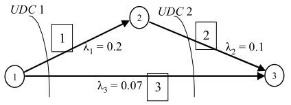
consider the project completed only when all tasks therein are completed.  Figure 1, below, 

provides a simple example.  Activity 2 cannot begin until activity 1 is completed.  Also, we 

consider the project completed only when all three activities have been completed; i.e. Node 

3 is realized. 

2 

3  1 

3 

1  2 

λ ₃ = 0.07 

λ ₂ = 0.1  λ ₁ = 0.2 

UDC1  UDC2 

We are given for each activity j its work content, Wj, representing the amount of work 

(effort, energy) to be done on the activity.  We assume that Wj is known in probabilistic 

terms (non­deterministic).  It is important to note that we consider the source of uncertainty 

to be internal to the project.  External uncertainty, such as that due to machine failure or 

weather, is beyond the scope of this research.  In general, work content is measured in some 

convenient unit depending on the activity and the resource; such as “worker­hours” or 

“computer­seconds”, etc. Consequently, only when the resource level is specified can we 

estimate the time to complete the activity.  This relationship depends on three entities: work 

content, resource level, and activity duration.  If a simple hyperbolic relationship is assumed 

then the activity duration is equal to the work content divided by the resource level, as we 

shall show in equation (2).  For instance, if the activity requires 36 worker­hours and 3 

workers are assigned to it, it shall consume 12 hours to accomplish.  However, if 4 workers 

are assigned to it, it shall require only 9 hours, etc.  We are also given a due date for the 

project, Ts, which is specified by the project “owner” and is known with certainty. 

We let xj represent the allocation of the resource to activityj.  It is important to note 

that the value ofxj is our decision variable while Wj is a random variable; thus we seek to 

find the best values of the xj variables that optimize the objective function.  We consider only 

one resource of unlimited availability, although in application the particular resource may 

vary from activity to activity within a project; i.e. one activity may require electricians as a 

resource while another may require bricklayers but no activity requires more than one 

(critical) resource at a time.  This could be accommodated in the proposed model by 

replicating the activity arc in parallel for each resource required for the represented activity 

Costs incurred in the execution of the project are of two forms: resource costs and 

lateness costs.  We assume a constant marginal cost for the resource,cR, and also assume that 

this cost is constant across all activities.  The latter assumption is made for ease of 

computation although it could be relaxed easily in the algorithm detailed in the next section. 

We are also given a cost of lateness for the project,cL per unit time of delay.  In our 

application, we normalize these costs by dividing through bycR.  Again, this assumption 

serves to simplify the computations; in any application more realistic costs would be known 

and could be used (such as piece­wise linear and convex costs).  If we let ¡ denote the time 

of project completion, a random variable, the cost of lateness is defined as cL (max{0,¡ – 

Ts}).  Finally, we seek to find an allocation vector,X, minimizing the sum of the expected 

value of these two costs. 

The first major assumption we make is the distribution function of each activity’s 

work content,Wj.  Because of its tractability and ease of use, we assume that Wj follows an 

exponential distribution with parameter λj: 

Wj ~ exp(λj), "j ÎA  (1) 

As we will show, this assumption will greatly decrease our computational burden because of 

the exponential distribution’s memory­less property.  Further, we assume that the resource 

allocation, xj, is bounded from below bylj and from above byuj: 

0< lj£ xj £uj < ¥ " Î,  j  A

Note that this assumption does not conflict with the earlier assumption of unlimited resource 

availability – it only constrains the resource allocation to any individual activity. We assume 

parallel at a given time.  Given our assumptions of exponential work content and bounded 

resource allocations we let Yj denote the duration of activityj: 

j  j 

j 

W  x 

Y =  (2) 

As Wj is exponentially distributed and xj is a decision variable, it can be easily 

demonstrated that Yj also follows an exponential distribution with parameter xjλj.  Note that 

this definition necessitates our bounding ofxj; without bounds onxj, the duration of activityj 

will not necessarily take on a meaningful value.  While the assumption that the duration of an 

activity takes on an exponential distribution may seem unreasonable, such a choice can be 

justified on three grounds. 

First, the memory­less property of the exponential distribution aids greatly in 

computation and, as we will show in section 3.2, lends well to the use of continuous time 

Markov chain (CTMC) theory for its analysis.  Second, and perhaps more importantly, the 

exponential distribution is the limit of the class of distributions known as “new better than 

used in expectation” (NBUE) distributions, to which all proposed distributions of activity 

durations known to us belong.  That is to say, if a task has not completed after ttime units, 

the expectation that the task will take 1/xjλj additional units provides an upper bound on the 

expected time the task should take in actuality.  Thus this assumption ensures that we provide 

an upper bound on the expected project duration and cost.  Lastly, using the exponential 

distribution and modeling the project as a CTMC can be considered the fundamental 

“building block” which serves other potential work content distributions.  This is due to the 

fact that any continuous distribution can be approximated to any desired degree of accuracy 

each “phase” is exponentially distributed – and we are back to the CTMC model based on 

these exponential distributions. 

Finally, we assume that the cost of resource allocation to activityj is quadratic in the 

allocation over the duration of the activity.  This reflects the added cost of employing 

additional resources.  It also could be considered representative of the law of diminishing 

marginal returns.  It also has the added advantage of resulting in a linear funcdtion of the 

allocationxj.  Thus the cost of resource allocation to activityj is defined as: 

2 

R R 

j _j  j j j 

C =c x Y = c x W .  (3) 

Therefore, the expected cost due to resource allocation to all the project activities is given by: 

[ ]  R 

a  R 

a  a 

C c 

ε

A 

x

l

Î

æ ö

= × _{ç ÷}

è ø

å

In order to properly evaluate the portion of the project cost due to lateness we must 

first establish the distribution of the project completion time.  To do so, we will first apply 

the principles established by Kulkarni and Adlakha [1986] to develop a continuous time 

Markov chain representative of the project network.  Next we present the known results from 

the Phase­Type Distributions in order to evaluate the density function of the project 

distribution. 

3.2  Continuous Time Markov Chains 

Kulkarni and Adlakha [1986] developed a methodology for transforming a project 

network with exponentially distributed activity completion times into a CTMC.  We will now 

We begin with a graphG = (N, A) representing the project in the AoA mode of 

representation as previously stated.  Without loss of generality, we assume that the project 

begins at time zero and will end at a randomly distributed later time, ¡, once all of the 

activities have been completed.  At a particular time, t, between 0 and ¡, each activity in A 

can be in one of three states: 

Active:  An activity is active if it is in process at time t. 

Dormant:  An activity is dormant if it is completed but at least one other activity 

ending at the same node is stillactive at time t. 

Idle:  An activity is idle if it is neither active nor dormant.  This includes all 

activities that are yet­to­be­initiated and those that are completed along 

with all other activities ending at the same node. 

Clearly, a project is completed when it has no active ordormant activities.  Since 

each activity is in one of these three states Kulkarni and Adlakha [1986] define the following 

sets for any time t ≥ 0: 

Y(t) = {a ÎA: ais active at time t}, 

Z(t) = {a ÎA: ais dormant at time t}, and the state of the project 

is given by: 

X(t) = (Y(t),Z(t)). 

The set of idle activities is the complement of the set X(t) inA.  Before proceeding further we 

must define a cutset.  Given a project graphG = (N, A) in AoA representation, let B be a 

proper, nonempty subset of the set of nodes, N, and  B  be its complement inN.  Further, we 

define  ( , )B B ={jÎA i: ÎB i, 'ΠB} where i and i' denote the start and end nodes of activity 

denotes the start node of a project (node 1) and n denotes the terminal node of the project, n 

= |N|.  Further, the cutset is a uniformly directed cutset (UDC) if no arcs extend from  B  into 

B, symbolically,  ( , )B B = Æ  .  The project in Figure 1 has 2 UDC’s, both of which are 

labeled. 

As stated by Kulkarni and Adlakha [1986], {X(t),t≥ 0} is a representation of the 

state of the project which forms a continuous time Markov chain (CTMC) with a single 

absorbing state when mutual independence of the activities is assumed.  This stems from the 

fact that X(t) forms a 2­partition of a UDC for all times t.  If we define S as the set of all 

admissible 2­partitions ofUDCs inG, then clearlyX(t)ÎS.  Whent ≥ ¡, the setsY(t) and Z(t) 

are both empty, thus X(t) = (Æ,Æ) and S =SÈ Æ Æ( ,   forms the state space for the CTMC. ) 

Generally,  S  is the set of all possible combinations ofactive and dormant activities of the 

project that can occur according to the precedence constraints, extended by the empty set, 

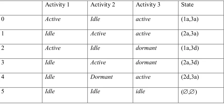
(Æ,Æ).  For the project in Figure 1,  S  contains 6 states, which are enumerated in Table 1.  A 

graphical representation of the CTMC is given in Figure 2: 

Table 1: State Space of the CTMC 

Activity 1  Activity 2  Activity 3  State 

0  Active  Idle  active  (1a,3a) 

1  Idle  Active  active  (2a,3a) 

2  Active  Idle  dormant  (1a,3d) 

3  Idle  Active  dormant  (2a,3d) 

4  Idle  Dormant  active  (2d,3a) 

5 

3  4 

2  1 

0 

(1a,3a)

Æ 

(2a,3d)  (2d,3a)  (2a,3a) 

(1a,3d)  λ ₂ 

λ ₃  λ ₁ 

λ ₃ 

λ ₂  λ ₃ 

Project start 

Project end 

Figure 2: The State Space of the Project of Figure 1: 

Graphical Representation of the six states of the CTMC 

A few observations made by Kulkarni and Adlakha [1986] are worthy of note due to 

their importance and relevance to our research.

·  Transitions in the CTMC correspond to the completion of activities in the project and 

their associated rates correspond to the parameters of the completion time 

distribution.  This directly implies that in our research, the transition rates within the 

CTMC are random variables of rates {xjλj}.

·  The state (Æ,Æ) corresponds to the completion of the project.  With no activities left 

to initiate or complete, no transitions are possible from this state and so (Æ,Æ) is the 

single absorbing state of the CTMC.

·  Since each activity is completed exactly once, each state of the CTMC may be visited 

only once.  Thus, the states ofS are transient and the states of  S  can be numbered so 

that the rate transition matrix is upper­triangular: |S |  = m and 

·  The number of states in {X(t), t≥ 0} is finite for projects with a finite number of 

activities.  Therefore, {X(t),t ≥ 0} will be completed in finite time with 

probability 1.

·  Finally, if | A | = a, the number of states in the CTMC follows: 

a £ |S | £ 2 a  (5) 

with the lower bound occurring when all activities of the project are in series and the 

upper bound occurring when all activities are in parallel. 

3.3  Phase­Type Distributions 

In order to establish the expected cost of lateness, we must first describe the 

distribution of time until the project’s completion.  Employing the CTMC interpretation of 

the model previously described the project can be considered completed when the Markov 

process reaches its absorbing state.  When an absorbing CTMC has a single absorbing state 

the distribution of time until absorption can be described by the phase­type (PH­type) 

distribution.  The phase­type distribution gets its name from the path taken by the project 

from initiation to completion, which can be viewed as a series of stages, or “phases,” each 

having an exponential distribution. 

The parameters of the phase­type distribution are a probability vector, (a,am+1), and 

the CTMC’s rate generator matrix: 

0  ( ) ( 1) 

(1 ) 0(1 1)  

m m m 

m 

T T  Q 

0

´ ´

´ ´

é ù

= ê ú

ë û 

Here, the T matrix is representative of the transient states of the matrix, withTii < 0 for 1 ≤i 

≤ m and Tij³ 0 for i≠ j.  Additionally: 

T 0 +Te =0,  (7) 

where e represents a column vector of dimension (1xm) and 0 is a vector of zeros of 

equivalent dimension; i.e. the rows of the matrixQ sum to 0.  As an example, the Q matrix 

for the project in Figure 1: 

0.27 0.20 0.07 0 0 0 

0 0.17 0 0.07 0.10 0 

0 0 0.2 0.20 0 0 

0 0 0 0.1 0 0.10 

0 0 0 0 0.07 0.07 

0 0 0 0 0 0 

Q

-

é ù

ê _- ú

ê ú

-

ê ú

= ê ú

-

ê ú

ê - ú

ê ú

ë û 

The vectora is an initial probability vector, also called the “counting probability” ofQ.  This 

vector represents the probability that the Markov process begins in a given state.  As such, 

we have: 

a ∙e +am+1 =1.  (8) 

For our purposes, we assume the project begins with no activities completed; i.e. the project 

is in the first state with probability 1.  Thus we have a =[1 0(1xm)]. 

In general, the PH­type distribution, hereby referred to as F(∙), can be represented by 

(a,T).  A necessary and sufficient condition for the states of the CTMC represented byT to 

be transient is that the matrixT is nonsingular.  As a result, T k® 0 as k ® µ.  When given 

an initial probability vector (a,am+1), the cumulative distribution function of the time to 

absorption in state m+1is given by: 

The evaluation ofe Tt has been studied in depth.  Traditionally, it is given by the 

Taylor series: 

1  !  0  ( )  T 

i  T

¥

=

=

å

t i 

ι 

e t  ,  (10) 

however, it can by calculated in a myriad of other ways as demonstrated by Moler and van 

Loan [2003]. 

A few observations about the PH­type distribution are now necessary for our 

research:

·  The functionF(∙) has a jump of height am+1 at t = 0.  This is equivalent to the 

probability that the process begins in the absorbing state.  For our research, this is 

somewhat irrelevant because we assume the project starts with no activities 

completed. In practice, this assumption could be relaxed in the interest of managerial 

flexibility; i.e. after a certain amount of time, the manager could re­optimize his or 

her resource allocation according to the progress of the project at that time.

·  The probability density function (pdf) f(∙) is given by: 

0  ( ) ( ) t  . 

t 

f t d F t e T 

d  α T

= = × ×  (11)

·  The expected value and variance of the PH­type distribution, respectively, are given 

by: 

–a ∙T ­1 ∙e and 2a∙T ­2 ∙e  (12) 

and, in general, the non­central moments fi ofF(∙) are given by:

3.4  The Cost Function 

The PH­type distribution can be used to formally state the cost function over which 

we seek to optimize.  As of the moment, we have in hand the expected cost of resource 

allocation, given by (4) above; it remains to derive the portion pertaining to the expected cost 

of lateness. 

First, as previously stated, the cost of lateness is defined byCL(¡ ) = cL (max{0,¡ – 

Ts}).  With the distribution of¡ following the PH­type distribution we must use integration 

to calculate the expected cost of lateness:  0  0  0  0  [ ] ( ) ( )  ( )  ( )  s  L L  t  L  t  s  T 

C C t f t  dt 

C t   e dt 

t­T   e dt 

ε

ò

ò

ò

It is important here to remember that the entries of the matrixT, as well as T 0 , are determined 

by the completion times of the activities in A.  Under our assumptions these completion times 

are functions of the resource allocations to the activities in the project.  Thus, the expected 

cost of lateness is also a function of the vector X.  In total, we seek to find the optimal 

resource allocationX to minimize the expected project cost: 

0 

[ ( )] L  ( ) 

s  a  _t  s  T  a  a 

C c t­T   eT  dt 

A 

x 

X  α T

l

e

å

ò

subject to the bounds on resource allocation as well as the precedence constraints expressed 

as nodes inG.  Here, the value cR has dropped out of the equation as it has been set equal to 1 

Chapter 4 

Description of Algorithm

In order to solve the problem at hand, we focus our research on a modified derivative descent 

algorithm.  We first compute an approximation to the partial derivative of the expected cost 

with respect to the allocation to each of the activities and then choose to modify the 

allocation to the activity that has the greatest negative derivative.  Next we use line search 

techniques to find the minimum expected cost allocation to the chosen activity while holding 

the other allocations constant.  The algorithm iterates using these two steps until a specified 

stopping criterion is met.  In order to execute any of these steps, we first must be able to 

compute the expected cost at a particular allocation. 

4.1  Cost Computation 

As previously described, the expected cost of the project (given in (15) and repeated 

here for convenience) contains two terms: 

0 

[ ( )] L  ( ) 

s 

a  _t 

s  T  a 

a 

C c t­T   eT  dt 

A 

x 

X  α T

l

e

Î

æ ö

= _{ç ÷} + × × × ×

è ø

å

ò

The first term relates exclusively to the level of resource allocation.  Since the work content 

distribution parameter, λi, is given for each activity the expected cost of resource allocation 

can be computed directly.  The second term, which relates to the lateness of the project with 

respect to a given due date,Ts, cannot be computed directly for the following reason.  Due to 

summation to approximate the expected cost of lateness.  Applying a summation requires 

assuming time takes on discrete values.  Azaron et al. [2007] arrive at the same conclusion 

through the use of control theory.  They take the approach of dividing the “time interval” 

(that is, the interval of time to project completion) into K portions of lengthΔt and solve a 

system of difference equations.  However, we choose to depart from this approach since the 

“time interval” is not known.  For example, a trivial project involving only a single activity 

will have a significantly shorter “time interval” when allocating 3 units of the resource than 

when allocating just 1 unit.  Instead, we set the length ofΔt and take the sum of lateness costs 

until the probability that the project takes longer thanm∙Δt time units is sufficiently small, 

sayplim.  Since the expectation of cost involves computing the probability that the project 

completes within a certain time interval, this method of calculation requires no additional 

computational steps. 

We, therefore, take a midpoint Riemann sum of the product to approximate the value 

of the integral.  For suitably small values ofΔt this method provides an excellent 

approximation.  The downside, however, is that while decreasing Δt to increase the precision 

of the approximation we also increase the computational burden.  We settle this tradeoff by 

letting Δt equal a fraction of the standard deviation of the project completion time provided it 

is greater than a lower bound, lΔt, as this helps to normalize the computational time for each 

instance in which the expected project cost is computed. 

The computational burden required by the cost calculation derives from the 

calculation of the probability that a project completes in a specified window of time.  Recall 

calculation of the expected cost, much can be gained if we let R = e T .  Equation (9) then 

becomes: 

F(t) = 1 –a ∙Rt  ∙e fort ³ 0.  (16) 

This computation requires computing R t rather thane Tt . 

The algorithm for computing the cost then proceeds as follows: 

Step 1: Initialization:  Let t =Ts, let Δt = max{z·σtn, lΔt} where tn denotes the project 

completion time and z is a predefined fraction, let CP = 0, let p0 denote the probability 

that the project completes before time Ts, i.e. let p0 = F(Ts), let Rmat= R t , and let U = 

R Δt . 

Step 2: Calculate the probability, p, that tn falls in the interval of [t,t+Δt]: 

p1 = F(t + Δt) = 1 –a∙Rmat ∙U ∙e  (17) 

p = p1 ­ p0  (18) 

Step 3: Let CP = CP + cL ∙ p∙ ((2t +Δt)/2 ­Ts).  Ifp1 exceeds 1­plim then go to Step 4. 

Otherwise let p0 =p1, let t = t+ Δt, let Rmat = Rmat ∙U, and repeat from Step 2. 

Step 4: Add the expected cost of resource usage to the expected lateness cost, CP, using (4) 

and stop.  CP now equals the expected total project cost. 

In the algorithm, we use U and Rmat in order to eliminate the need to calculate the power of 

an exponential in each step.  Instead, we calculate these quantities once (from knowledge of 

the Wj’s and the resource allocation) and can then rely on matrix multiplication, which is 

significantly less burdensome computationally than matrix exponentiation. 

With an effective way to calculate the total expected project cost in hand, we can now 

4.2  Selecting Candidate Activities 

In general, our algorithm optimizes the project cost by changing the allocation to one 

activity at­a­time.  We now need to explain the procedure to select activities that are the best 

candidates for optimization.  The best candidates in our procedure are those that could lead to 

the greatest decrease in expected project cost. 

The two terms of the project cost behave diametrically opposite in their response to 

changing resource allocations.  The project resource cost increases linearly with respect to an 

increase in resource allocation to any activity.  On the other hand, increased resource 

allocation to the activities tends to shorten their expected duration and so the expected 

lateness cost would decrease with respect to such a change in allocation.  A decrease in 

overall cost, therefore, could be obtained from either a decrease or an increase in resource 

allocation. 

An important observation is that the expected project cost is a convex function with 

respect to the allocation to a single activity.  This fact is a result of the two convex 

components of cost.  The expected cost of lateness decreases convexly due to the exponential 

distributions on which it is based.  Further, since the resource costs are linear (hence convex) 

in the resource allocation, the sum of the two costs is convex.  Thus, repeatedly optimizing 

allocations to single activities one­at­a­time will descend monotonically to reach the optimal 

solution. 

Since no analytical expression is known for the partial derivative of the cost function 

with respect to the allocation to any activityaj, we must rely on approximations to proceed. 

Such an approximation would enable us to select the activities to which a change in 

associated with a small change in allocation, d, to a particular activity we can approximate 

the derivative of the cost function by first taking the difference between this cost and the cost 

of the initial resource allocation and then dividing by the magnitude ofd.  Since a decrease in 

cost can occur via an increase or a decrease in allocation, and thanks to the convexity of the 

cost function, the best candidate allocations are those with the steepest derivatives causing a 

decrease in cost.  Further, ifd is constant across all activities, we can simply find the change 

in allocation reflecting the greatest decrease in cost, as we are not concerned with the actual 

value of the derivatives, but rather their magnitudes with respect to one another. 

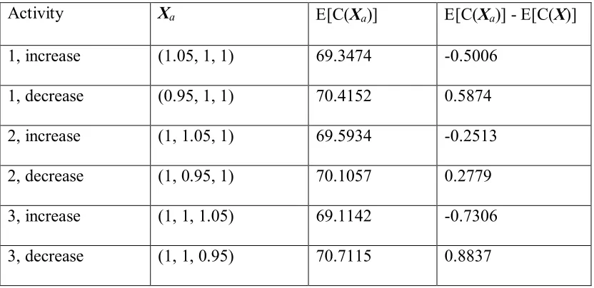
Letting X+a = X+d∙ea, where ea is a vector of dimension |A| with zeros everywhere 

except in positiona, denote the allocationX with the value of the ath allocation increased by 

the amount d, further we allow X­a = X – d∙ea to denote the allocation with the ath allocation 

decreased.  We calculate E[C(X+a)] and E[C(X­a)] for each activity.  Withe[C(X)] in hand, 

we find E[C(X+a)] –E[C(X)] and E[C(X­a)] –E[C(X)] for each activity, a, and use this as a 

surrogate for the value of the derivatives of the cost function with respect to the allocation to 

a.  We select the activity corresponding to the greatest decrease in cost as the candidate 

activity.  If the decrease in cost comes fromX+a the allocation to activitya must be increased. 

Likewise, if this comes fromX­a we must decrease the allocation to activitya.  Since we are 

dealing with minimization of the cost function, for certain network structures both increasing 

and decreasing the allocation can cause an increase in cost.  Thus it is important to check 

both an increase and decrease in allocation rather than assuming that an increase in cost in 

4.3  Improving Computational Efficiency 

As with computing the cost function, approximating its derivative can be 

computationally burdensome, considering that we must calculate E[C(X+a)] and E[C(X­a)] for 

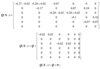
each activity.  We let Q(X+a) represent the matrix Q with the allocation to activitya increased 

by the value d.  Note that increasing the allocation to a single activity may correspond to 

increasing the value of several entries in the originalQ matrix, as well as the decreasing their 

corresponding elements along the main diagonal.  Changing the allocation to activityi byd 

implies that we must change the values in the Q matrix bydli.  This change can be viewed 

as matrix addition.  These facts are best illustrated with an example from the project in 

Figure 1, where we change the allocation to activity 1 (li = 0.2) withd= 0.1: 

1 

0.27 0.02 0.20 0.02 0.07 0 0 0 

0 0.17 0 0.07 0.10 0 

0 0 0.20 0.02 0.20 0.02 0 0 

( ) 

0 0 0 0.1 0 0.10 

0 0 0 0 0.07 0.07 

0 0 0 0 0 0 

Q X - - + é ù ê _- ú ê ú - - + ê ú = ê ú - ê ú ê - ú ê ú ë û  +  1 

0.02 0.02 0 0 0 0 

0 0 0 0 0 0 

0 0 0.02 0.02 0 0 

( ) 

0 0 0 0 0 0 

0 0 0 0 0 0 

0 0 0 0 0 0 

Q X Q

- é ù ê ú ê ú - ê ú = _{+ ê ú} ê ú ê ú ê ú ë û  +  1 1  ( ) 

Q X+ =Q+ F + 

where, F+a represents the matrix corresponding to the increase in allocation to activitya. 

Recall from elementary matrix algebra that e A+B = e A ∙e B whenA and B are 

commutative: A∙B = B∙A.  Unfortunately for our purposes, Q ∙Fa¹ Fa ∙Q.  However, the 

sparse nature of the Fa matrix implies that these two terms are approximately equal.  Further, 

eFa is nearly equal to the identity matrix, I.  With these facts in mind, we can use e Q+Fa = e Q ∙ 

eFa or rather the transient matrices e T+fa = e T ∙efa , where fa denotes the transient portion of

Fa, for use as an approximation in the density function of the completion time distribution. 

This approximation provides a good indicator of the derivative of the cost function with 

respect to direction (as in whether increasing the allocation leads to an increase or a decrease 

in cost) as well as the magnitude of the change in cost.  We will validate this approximation 

in the next section by comparing the expected costs returned by the algorithm when using the 

approximation and the exact determinations of the cost derivatives.  Note that this analysis 

can be applied to the computation ofE[C(X­a)]. 

The key advantage this approximation provides is that it eliminates the need to 

calculate the matrix exponential for the evaluation of the derivative at each iteration.  Since

Fa does not depend on the current allocation, the efa matrices can be computed once at the 

beginning of the algorithm and stored for use throughout the optimization process.  Since e T 

is needed for calculating the cost at each iteration this matrix is in hand as well.  Thus, e T ∙efa 

is computed and passed to the cost calculation algorithm as the matrix, R. 

4.4  Optimizing The Allocation to a Single Variable 

With a candidate variable in hand, we now seek to optimize the allocation of 

stated, the expected project cost is a convex function with respect to the allocation to a single 

activity.  Any convex optimization procedure could therefore be applicable here. However, 

due to the difficulty involved in finding exact analytical expressions for the partial 

derivatives of the cost function, we opt to use Fibonacci search as our method of determining 

the optimal allocation to the selected activity.  Note that this “optimal” allocation is “locally 

optimal” in a sense as it depends upon the allocation to the other activities. 

At its core, Fibonacci search, often referred to as “golden mean” search, finds the 

optimal point in a range of feasible values by repetitively shrinking the range, stopping when 

the range is sufficiently small to suggest a single optimal point.  Fibonacci search makes use 

of the so­called “golden ratio," which Wilde [1964] shows is the most computationally 

efficient method of finding the optimal value of a variable when searching along a line. 

Given a lower bound, l, and an upper bound, u, on the range, two new points are calculated 

within the range: ml andmu where ml < mu.  We define r as the inverse of the “golden ratio” 

and use r to give values for ml and mu: 

2 

0.618  1 5 

r = »

+  (19) 

ml =l∙ (r) +u∙ (1 – r)  (20) 

mu = l∙ (1 – r) + u∙ (r).  (21) 

For our purposes, these points represent different resource allocations.  If activityj was 

selected as the candidate activity and its cost decreases with increased allocation we let l be 

the current allocation and let u be uj for activityj while keeping the allocations to the other 

activities unchanged.  If its cost decreases with decreased allocation, we define the upper 

bound as the current allocation and let lj be the lower bound on the allocation to activityj. 

with lower and upper bounds defined at 1 and 3 respectively.  If activity 1 is selected as the 

candidate activity and its cost decreases with increased allocation we let l= X  (the current 

allocation) and u = (3, 2, 2).  Conversely, if the cost increases with increased allocation, let l 

=(1, 2, 2) and u =X.  Values forml and mu are then defined by (20) and (21) respectively. 

With these four values in hand (l, u,ml, and mu), we recursively redefine the bounds 

on the range to hone our search to the minimum expected cost allocation.  Optimization 

proceeds by first calculating the expected costs of allocations ml andmu.  The convexity of 

the expected cost function allows us to conclude that the minimum falls between the greater 

of the two values and the opposite absolute bound; i.e. ifE[C(ml)] <E[C(mu)] then the 

optimal value must lie betweenl and mu, otherwise E[C(ml)] >E[C(mu)] and the optimal 

value must lie betweenml and u.  If the two expected costs are equal, either bound can be 

used.  Using these values we redefine the bounds on optimization using the absolute bound 

nearer ml ormu corresponding the lower cost and redefine the opposite bound as ml ormu 

corresponding the greater expected cost.  The two points within the range are then redefined; 

however, the use of the “golden ratio” permits calculation of only one of these points.  The 

ml ormu corresponding to the lower expected cost will take the value of the opposite 

midpoint in the next iteration, as the use of equation (20) or (21) will yield this value. 

Further, only one new expected cost must be calculated in each iteration.  As an example, 

suppose E[C(ml)] <E[C(mu)].  In the next iteration, l will remain unchanged, u will take the 

previous value ofmu,mu will take the previous value ofml, and a new ml can be calculated 

using (20).  These concepts are illustrated numerically in Section4.6 below. 

In each iteration, we shrink the search range by the ratio r as defined in (19), 

interval exists betweenl and